Sage Journals: Discover world-class research

Abstract

We use a graph convolutional neural network (GCN) for regional development prediction with population, railway network density, and road network density of each municipality as development indicators. By structuring the long-term time series data from 2833 municipalities in Switzerland during the years 1910–2000 as graphs over time, the GCN model interprets the indicators as node features and produces an acceptable prediction accuracy on their future values. Moreover, SHapley Additive exPlanations (SHAPs) are used to make the results of this approach explainable. We develop an algorithm to obtain SHAP values for the GCN and a sensitivity indicator to quantify the marginal contributions of the node features. This explainable GCN with SHAP decomposes the indicator into the contribution by the previous status of the municipality itself and the influence from other municipalities. We show that this provides valuable insights into understanding the history of regional development. Specifically, the results demonstrate that the impacts of geographical and economic constraints and urban sprawl on regional development vary significantly between municipalities and that the constraints are more important in the early 20th century. The model is able to include more information and can be applied to other regions and countries.

Keywords

Regional development prediction GCN SHAP long-term data explainable deep learning

Introduction

Regional development is the result of interaction among various factors. Population concentrations arise due to job opportunities, and, in turn, the increasing travel demand induces extensions to the transportation services. There are a wide range of models to describe these dynamics. Most land-use interaction models use detailed information and do not focus on long-term regional development. Instead, data-driven approaches usually rely on regression approaches. In this research, we explain the cyclic relationship between population concentration and transport infrastructure development considering the transportation network structure over a period of 100 years by a graph convolutional approach. As part of this, and in order to gain insights into the differences between influential factors in different regions and different periods, we derive SHapley Additive exPlanation (SHAP) values to interpret this deep learning model.

Our motivation to use a graph-based approach is based on the hypothesis that it is the connectedness and attributes of cities in the vicinity and the infrastructure itself that influence regional development. Graph convolutional networks (GCNs) can incorporate information from neighboring connected nodes to the target node. They have been widely applied to many real-world phenomena that can be represented as graph structures, including biology studies and work on social networks (Wu et al., 2019). GCN approaches are also applied for transportation network studies. In particular, there are a range of studies on short-term traffic prediction. As an exemplary approach, we refer to Lee and Rhee (2020) who use a graph with multiple attributes, as was also done in this study. Further, Yu et al. (2018) predict short-term traffic flow and speed with convolution performed on the spatial and temporal dimension. An approach for general demand forecasting using a spatio–temporal convolutional approach is proposed by Wang et al. (2018) and applied to ride-sourcing data. Another stream of research uses image-processing methods for transport problems. Recently, Bapaume et al. (2021) utilized a GCN approach to forecast metro train loads. The line loadings of the metro system are represented as an image based on the time-space diagram of the trains with colors representing loads at a station for specific run. To the best of our knowledge, graph convolutional approaches have, however, not been used to model long-term regional development.

The paper is organized as follows. After this introduction, we review the literature on land-use models and research using historic time-series data to predict urban developments. In “Graph convolutional learning framework”, we introduce our general proposed deep learning model framework, and in “Interpretation with SHAP values”, we introduce an adaptation of SHAP for result interpretation. Between these two sections, in “Model inputs”, we discuss our input data. We put this section ahead of “Interpretation with SHAP values” as it allows us to better illustrate the kind of SHAP values that we obtained. “Switzerland case study” then describes the prediction results and model interpretation using a century of Swiss data. This is followed by the conclusions.

Long-term transport land-use interaction studies

Various types of models have been developed for predicting urban or regional development to help city planners and policy makers to simulate different scenarios and estimate the influences of policies and strategies. Three typical types of urban/regional growth models dominate: land use-transport interaction (LUTI) models, agent-based models, and cellular automata (CA)-based models (Li and Gong, 2016).

An LUTI models the population, land-use, transport, and travel demand interactions seen as a reciprocal process subject to the spatial and temporal constraints such as government budgets, technical limitations, and topographical obstacles; see Xie and Levinson (2011) for an example and more detailed discussion. Agent-based models can flexibly describe a system from the behavior of components that are involved and have been applied in a diverse range of topics (Chen, 2012; Waddell, 2002). In the field of urban planning, it uses real drivers of land-use change and looks into the interaction among those drivers of urban development. This type of model has been implemented in some platforms such as “Swarm”. While LUTI and agent-based models are usually applied at local scales with detailed datasets, CA models can be applied at regional scales and use more general datasets such as terrain, land-use maps, transport networks, or locations instead of actual drivers for urban/regional growth (Li and Gong, 2016). The basis for these models is the definition of grid cells that evolve according to certain transition rules based on the states of adjacent cells (Otgonbayar et al., 2018).

Instead of the above-described simulation or model approaches, data-driven approaches based on time-series data and regression analysis have also been gaining popularity. Our case study is based on the Swiss data that have been used by Tschopp et al. (2006) and Fuhrer (2019). These studies have been using accessibility derived from historical time series data of the Swiss transportation networks together with historical records of traveling speed to quantify the long-term influences of the transport system. Tschopp et al. (2006) discuss the impact of accessibility on the demographics and the economy of Swiss municipalities for the years 1950–2000 using multi-level regression analysis. Fuhrer’s work studies the time period from 1720 to 2010. The work discusses a method to construct the historical transportation networks and to calculate accessibility and productivity impacts for the different time periods. Another historic study is the one by Li et al. (2021). Their work looks at the impact of accessibility for population dynamics during the Sui-Tang period in the 7th and 8th century. The study points out the importance of the Grand Canal and describes accessibility as an amplifier for the population dynamics caused by wars. Among work using more detailed data from the 19th and 20th century, we refer to Lahoorpoor and Levinson (2019) who described a positive feedback between tram development and population growth in different districts of Sydney. Akgüngür et al. (2011) described the positive effect of the rail expansion in the Ottoman Empire on population distribution and economic development using correlation analysis. Further studies on rail expansion and development in Europe have been carried out by Kasraian et al. (2016a) and Mimeur et al. (2018). For a full review of empirical studies using long-term historical data and its land-use impacts, we refer to the review paper of Kasraian et al. (2016b). To the best of our knowledge, none of these studies has used a graph-based machine learning approach to understand the relationship between accessibility and population development, which is the focus of this study.

Graph convolutional learning framework

We define municipalities as nodes with features and relations among municipalities as edges. The number of nodes is fixed while node features and edges change over time. For each time step $t$ , it can be expressed as an undirected graph $G_{t} = (V, ℰ_{t})$ , with $N$ nodes $v_{i \in {1,2, \dots, N}} \in V$ and $R$ types of edges ${(v_{i}, v_{j})}_{t}^{(r)} |_{r \in {1,2, \dots R}} \in ℰ_{t}$ . The size of the network corresponds to the number of municipalities and can be large. As discussed further in “Switzerland case study”, in our case $N = 2833$ .

Each node has $F$ features, and the node feature matrix for the graph is denoted as $X_{t} \in ℝ^{N \times F}$ . This matrix inputs the attributes of the node to the model. The attributes can come from a wide range of indicators of regional development such as population, transportation network density, and economic indicators. A specific node feature vector for all nodes can be written as $x_{k, t} \in ℝ^{N \times 1}$ , $k \in {1,2, \dots, F}$ . Specifically, $x_{i, k, t}$ denotes the $k^{th}$ node feature of node $i$ at time $t$ . Edges can be written as $R$ weighted adjacency matrices $A_{t}^{r} \in ℝ^{N \times N}$ where $t$ is the time step and $r \in {1,2, \dots, R}$ denotes the type of relation. These adjacency matrices are further model input and describe the transportation network and its quality in terms of travel time between the nodes.

The structure of the deep learning model with its different building blocks is shown in Figure 1. The model consists of two repeating blocks where each block contains one graph convolutional layer (GraphConv) and one “GraphU-net” layer, a jumping knowledge layer and a linear output layer. In Supplemental Material, we describe the key features of these layers and refer to the literature for detailed further discussion.

Figure 1.

Deep learning model structure.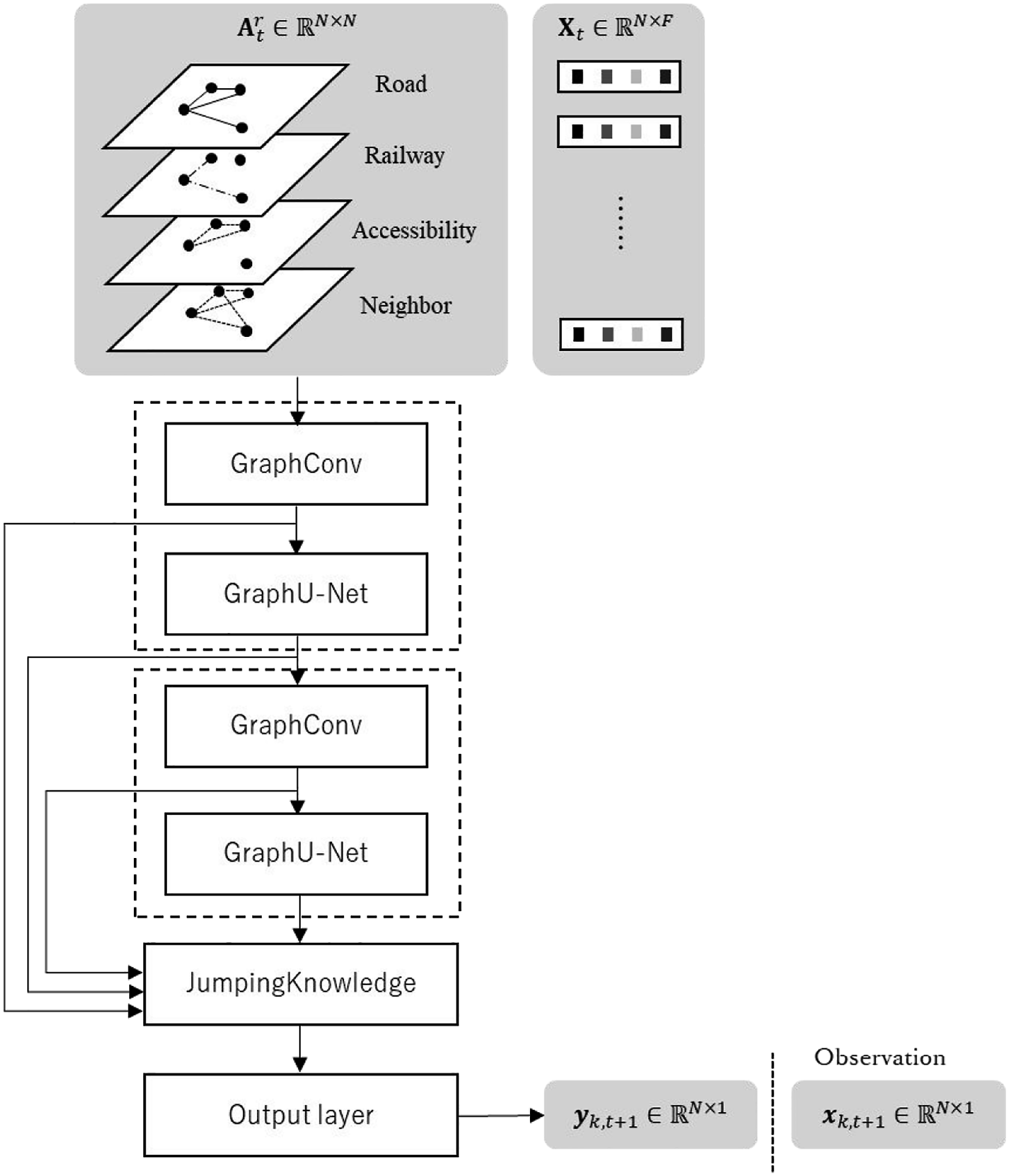

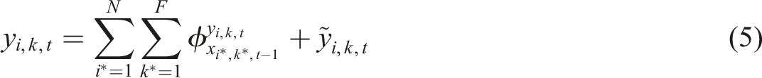
This framework can be applied to learn any of the F node features. It is important to note that each feature is learned with separate model runs as the resulting output of this model is an $N \times 1$ vector $y_{k, t + 1}$ , which are the predictions of one among the F node feature types for every single node in the next time step. The model fit in each iteration is evaluated with “loss”, which is defined as the mean square error (MSE) of this output compared to observed values. For the training, the Adam optimizer (Kingma and Ba, 2017) is used.

Model inputs

Overview

The abovementioned model framework is flexible to handle a range of input data. Which data are chosen for the node feature matrix $X_{t}$ and the adjacency matrices $A_{t}^{r}$ will be determined by data availability and the modeler’s judgment on what municipality characteristics as well as relations between these are likely to be significant. In our Switzerland application, four types of node attributes are employed. They are population, railway network density, road network density, and the difficulty to develop the transportation network considering the topographical and economic conditions within the municipality. Further, four types of edges are selected to describe the connection between two municipalities: railway connection, road connection, travel cost, and bordering status. Therefore, we have $X_{t} \in ℝ^{2833 \times 4}$ and $R = 4$ . The details to obtain the value for each node and edge feature will be elaborated hereinafter.

Edge types: Physical connections and accessibility relations

The four types of edges (relations) are shown in Figure 2. Figure 2(a) illustrates a transportation network with physical connections such as railway lines and roads; Figure 2(b) shows the accessibility relations based on a gravity model, in which the greater the width of the lines, the stronger the relationships between municipalities with lower travel cost for railway and road; and Figure 2(c) shows the connections between neighboring municipalities. These edges are added with the hypothesis that closer municipalities are more likely to have interactions independent of accessibility between these. The neighboring edges are constructed by considering the shared boundaries between polygons of municipalities as edges.

Figure 2.

Relations between municipalities in regional development (a) based on transport infrastructure, (b) based on accessibility, and (c) based on political boundaries.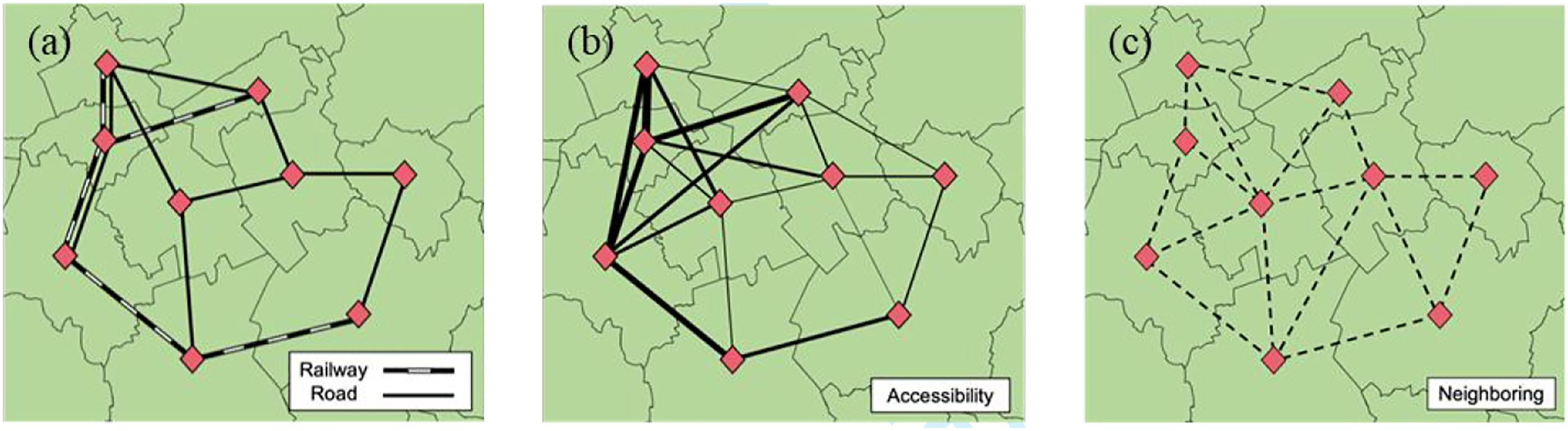

Transportation links that cross the boundary between two municipalities are regarded as edges connecting them. If there are multiple transportation links crossing the boundary between the same pair of nodes when transforming edge connections into an adjacency matrix, then the number of links will be accumulated as the weight in the adjacency matrix to show a stronger transportation connection (see Supplemental Material Figure S1 for an illustration).

We further use cost functions to travel between any single pair to measure the ease of access from $i$ to $j$ . This measure will be the weight of the connection between the corresponding OD, and we call this the “accessibility connection”, $w_{i j}^{u}$ , by mode $u \in {r a i l, r o a d}$ . We expect that two municipalities are more likely to have a stronger relation when the travel cost between them is lower. Following Yu et al. (2018), we formulate this resembling a gravity model as in (1) with $w_{i j}^{u}$ values lower than 0.5 being set to zero, indicating that for these cities there is no relationship.

w_{i j}^{u} = exp (- 0.01 {(c_{i j}^{u})}^{2})

(1)

Node features: Population and network density

Recall that $x_{i, k, t}$ denotes the $k^{th}$ node feature of node $i$ at time $t$ . The first node feature is its population obtained directly from the data, so we let $x_{i, 1, t}$ denote the population of node $i$ at time $t$ . The second and third features describe the quality of the rail and road network considering their infrastructure length and capacity, dividing this term by the size of the municipality for which they are measured. We refer to these as “road network density” and “railway network density” even though these are weighted terms and have different units. Omitting the time step, the density indicators $x_{i, 2}$ for railway network and $x_{i, 3}$ for road network can be obtained from equation (2) as follows

x_{i, k \in {2,3}} = \frac{ρ_{m (j)}^{u \in {r a i l, r o a d}}}{d_{i_{c} j}^{2}} with j for which d_{i_{c} j} is the minimum

(2)

Here, $d_{i_{c} j}$ is the distance from the population centroid of municipality $i$ , denoted as $i_{c}$ , to the closest railway station or road access $j$ . The indices $ρ_{m (j)}^{r a i l}$ and $ρ_{m (j)}^{r o a d}$ indicate the capacity of transportation links passing municipality $m$ that contains the closest transport node $j$ . The equation to obtain $ρ_{m (j)}^{u}$ is

ρ_{m (j)}^{u} = \frac{\sum_{n \in N_{m (j)}} l_{n} v_{n}}{s_{m (j)}}

(3)where

N_{m (j)}

is the set of transportation links passing through the polygon of municipality

m (j)

l_{n}

is the length of transportation link

n

that belongs to

N_{m (j)}

, and

s_{m (j)}

is the area of municipality

m (j)

v_{n}

have different meanings for

ρ_{m (j)}^{r a i l}

and

ρ_{m (j)}^{r o a d}

. For the road network,

v_{n}

is the free flow speed of road

n

. For the railway network, it denotes the number of tracks of railway link,

n

, as we find in the tests that the number of tracks is more meaningful than the speed in the case of railway. The unit of the weighted railway network density is [1/m] and that of the weighted road network density is [1000/h]. Supplemental Figure S2 in the Supplemental Material provides a graphical illustration.

Node feature “Topographical Difficulty”

Regional development has constraints and is not uniform. The proposed reciprocal relationship between transportation and population development will be faster and more evident when fewer geographical, economic, and technical constraints are present. In mountainous countries, such as Switzerland, the population distribution at any point in history will clearly be influenced by the topography. To control for this, we use GIS data to extract the slope in each mesh utilizing the digital elevation model. We sum up the slopes for all meshes within the polygon of a municipality and then divide by the area of that municipality to obtain the average slope.

Furthermore, we consider that at the beginning of the last century, it would have taken longer and would require proportionately more resources to adjust the transportation network to population developments. Given limitations on available data, we suggest that Gross National Income (GNI) can, to some degree, reflect both the economic and technological capability of a country. Considering both topographical obstacles and technological capabilities as one factor constraining (the speed of) regional development, we refer to it as “difficulty” in the sense of “difficulty of developing the transportation infrastructure”. The hypothesis is that more mountainous regions and periods with less GNI will constrain the regional development. Difficulty is our fourth node feature for each municipality $i$ at time $t$ as in equation (4)

x_{i, 4, t} = \frac{δ_{i}}{\log_{10} G_{t}}

(4)where

δ_{i}

is the average slope in degree in the area of municipality

i

. Different model forms were tested, and we found that a log-scaled transform of GNI at time

t

denoted as

G_{t}

is most appropriate to express the gradual increase in technological capability over the century long analysis period. Hence, the unit of difficulty is [geographical slope/$], which expresses the financial resources available to overcome geographical height differences.

Interpretation with SHAP values

To interpret the “black box” deep learning model, we apply “SHapley Additive exPlanations” (SHAPs) proposed by Lundberg and Lee (2017). If adapting the original concept of Shapley values in game theory to machine learning prediction models, each input feature value of the instance is equivalent to a player in the game, and the output from the prediction model is the payout. Although SHAP values are increasingly used in a wide range of applications using, for example, gradient boosting regression or other machine learning approaches, the difference to our case is the application within the context of a network structure. The explanatory model used in this research is based on DeepExplainer (Lundberg and Lee, 2017). However, DeepExplainer is not applicable for handling deep learning models with graph structured data. Therefore, we used a modified DeepExplainer called GraphExplainer that generates plenty of reference inputs by random permutation of the original input (Fukuda, 2020).

With the concept of SHAP values and GraphExplainer, each input feature can claim its contribution to the predicted value. Let $ϕ_{x_{i^{*}, k^{*}, t - 1}}^{y_{i, k, t}}$ denote a specific SHAP value. It measures the actual amount in the predicted $y_{i, k, t}$ that should be attributed to $x_{i^{*}, k^{*}, t - 1}$ . It is interpreted as the contribution made by the $k^{* th}$ feature of node $i^{*}$ at time $t - 1$ to the prediction of the $k^{th}$ feature of node $i$ at time $t .$ We have $i, i^{*} \in {1,2, \dots, 2833}$ , $k \in {1,2,3}$ , $k^{*} \in {1,2,3,4}$ , and $ϕ^{y_{i, k, t}} \in ℝ^{N \times F}$ . According to the additive nature of SHAP, we can write the predicted value for the $k^{th}$ feature of node $i$ at time $t$ as the product of the sum of SHAPs and the baseline as in (5). It is important to note that $i^{*}$ can take the same value as $i$ . In this case, $ϕ_{x_{i, k^{*}, t - 1}}^{y_{i, k, t}}$ is termed “self-SHAP” and defines the contribution made by the $k^{* th}$ feature of node $i^{*}$ itself in the previous time step. Hence, in particular in slowly changing networks, it is expected to have a larger magnitude than the SHAPs of other nodes, which we term “influential-SHAP”. For better interpretability of the results, we distinguish the sum of self-SHAPs and the sum of influential-SHAPs in (6). The first term on the right of (6) is the sum of the four self-SHAPs of the node features, and the second term is the sum of influential-SHAPs of the features of other nodes. In addition, the “reference output” ${\tilde{y}}_{i, k, t}$ is on the right of (6). It is the expected output regardless of the input features of any instance and is obtained as the mean from 100 runs in which the elements of each input vector $x_{k \in {1,2,3,4}, t}$ are randomly shuffled among the nodes. The pseudocode of GraphExplainer can be found in Supplemental Material for “Interpretation with SHAP values”. It should be noted that producing SHAPs is time-consuming. It takes around 80 sc for a computer equipped with the Graphics Processing Unit (GPU) GeForce RTX 3060 Ti to produce $ϕ^{y_{i, k, t}} \in ℝ^{2833 \times 4}$ for one prediction value $y_{i, k, t}$ so that it requires more than 60 h to obtain all the SHAPs for predicting a specific vector $y_{k, t}$ .

Finally, we propose a novel indicator derived from self-SHAPs to measure the sensitivity of the prediction output to the changes in the input self-feature. The sensitivity to the features of other nodes is excluded from the discussion as the magnitude of influential-SHAPs is found to be much smaller. Let $β_{i, k^{*}, t - 1}^{k, t}$ denote the marginal contribution of the $k^{* th}$ feature of node $i$ in year $t - 1$ to the predicted $y_{i, k, t}$ . With this we obtain the marginal contribution as in (7): The output $y_{i, k, t}$ will change $β_{i, k^{*}, t - 1}^{k, t}$ units according to a unit difference between the $k^{* th}$ feature of the node itself and the mean of the $k^{* th}$ feature of all nodes in the input year. It is necessary to subtract the feature mean ${\bar{x}}_{k^{*}, t - 1}$ from the input feature because SHAP is the value added given this network feature mean. This sensitivity indicator is in analogy to the conventional definition of marginal contribution and is designed to allow for a comparison between this black-box deep-learning approach and a regression analysis, but it differs from linear regression coefficients in two aspects. First, the marginal contribution is prediction-specific, namely, it is only valid for a specific testing pair of input year and output year and may change for another pair. Second, it is node-dependent so that it describes the sensitivity of a specific feature for a specific node. To illustrate the advantages of this “explainable” GCN with SHAP, a multiple linear regression model (LR) is developed using the four lagged self-features as the independent variables. The LR model can be written as in equation (8). To conclude, ${\tilde{β}}_{k^{*}}^{k}$ , is the marginal contribution of the $k^{* th}$ feature in the prediction of the $k^{th}$ feature in a linear regression analysis. It is scalar and identical for every node and year. Differently, we have $β_{k^{*}, t - 1}^{k, t} \in ℝ^{N \times 1}$ for a specific test with year $t - 1$ as the input year and $t$ as the output year in this GCN framework. A numerical comparison with regression model results is provided in “Switzerland case study”.

y_{i, k, t} = \sum_{i^{*} = 1}^{N} \sum_{k^{*} = 1}^{F} ϕ_{x_{i^{*}, k^{*}, t - 1}}^{y_{i, k, t}} + {\tilde{y}}_{i, k, t}

(5)

y_{i, k, t} = \sum_{k^{*} = 1}^{F} ϕ_{x_{i, k^{*}, t - 1}}^{y_{i, k, t}} + \sum_{i^{*} \neq i} \sum_{k^{*} = 1}^{F} ϕ_{x_{i^{*}, k^{*}, t - 1}}^{y_{i, k, t}} + {\tilde{y}}_{i, k, t}

(6)

β_{i, k^{*}, t - 1}^{k, t} = \frac{ϕ_{x_{i, k^{*}, t - 1}}^{y_{i, k, t}}}{x_{i, k^{*}, t - 1} - {\bar{x}}_{k^{*}, t - 1}}

(7)

y_{i, k, t} = \sum_{k^{*} = 1}^{F} x_{i, k^{*}, t - 1} {\tilde{β}}_{k^{*}}^{k} + {\tilde{β}}_{0}^{k} + ε

(8)

Switzerland case study

Data from Switzerland

We applied the framework explained in the previous sections to the long-term time series infrastructure and population data of Switzerland. These are network data for the years 1910, 1930, 1950, 1960, 1970, 1980, 1990, and 2000. The resident population for each municipality in Switzerland was obtained from the Federal Population Census. The network and population data were obtained from a VISUM model that has been previously used in, for example, Fröhlich et al. (2006) and Axhausen and Hurni (2005). Gross National Income (GNI) shown in Supplemental Material Table S1 was collected from Bairoch (1976) and open data were provided by The World Bank (2020).

For the “topographical difficulty,” we used the 200-meter grid digital elevation model from the Federal Office of Topography “swisstopo” and a map of Swiss municipalities. We extracted the slope and calculated the average slope for each municipality. The map data were also utilized to extract the length of the transportation infrastructure that passes through each municipality. We used 2833 municipalities for which the abovementioned information is complete (see Supplemental Material Figures S4 to S7 for illustrations of the input data).

Model performance and interpretation

As shown in Table 1, we paired the data from two time-steps having an interval of 20 years as input and ground truth, respectively. Six pairs of data were obtained and split into four pairs for training and two pairs for testing: Split patterns A and B. For pattern A, we used the four pairs in the early years to train the model and tested the prediction capability with the two pairs in later years; vice versa for B. The prediction performance was tested for the population, rail-network density, and road-network density. Convergence was achieved, in general, before 1000 epochs for each of these predictions. An epoch denotes the iteration of the loop over both sets of GraphConv and GraphU-Net blocks in Figure 1 to train the model. The computational cost of one epoch was around 3 s with the aforementioned GPU. Tables 2 and 3 report the prediction results with a comparison between GCN and LR for both split patterns.

Table 1.

Training and testing data for the model.

	(1)	(2)	(3)	(4)	(5)	(6)
Input year	1910	1930	1950	1960	1970	1980
Output year	1930	1950	1970	1980	1990	2000
Split pattern A	Training				Testing
Split pattern B	Testing		Training

Table 2.

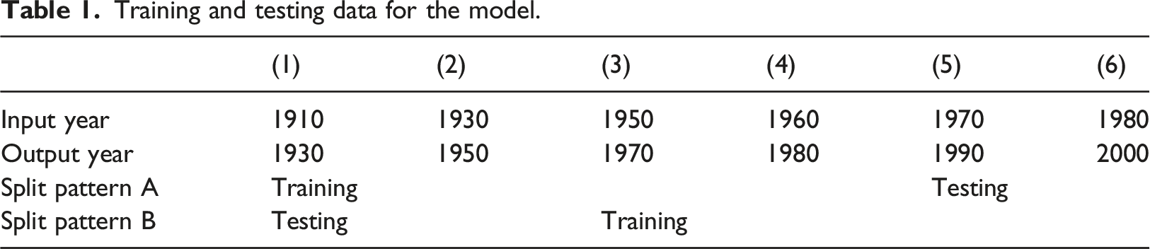
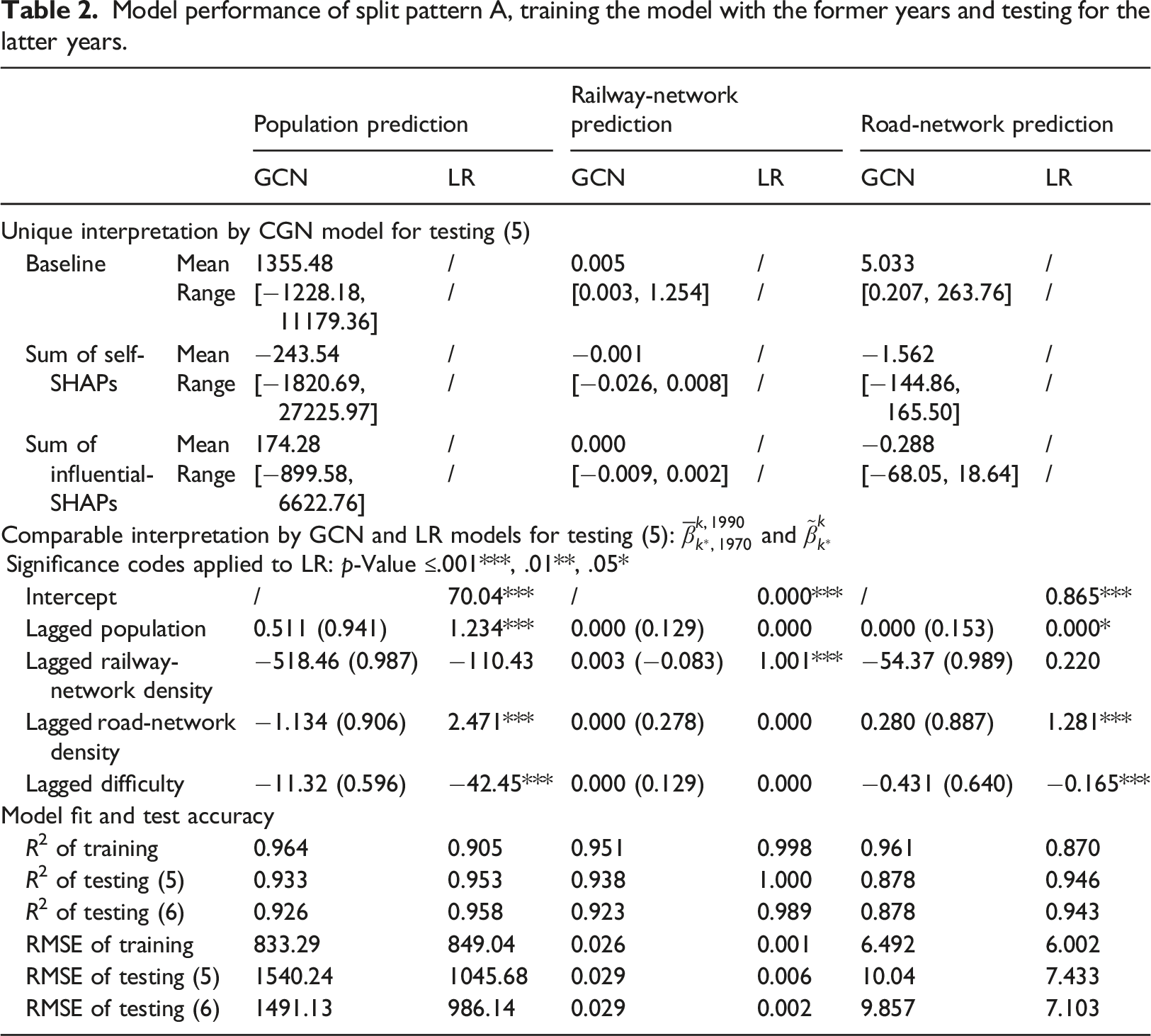
Model performance of split pattern A, training the model with the former years and testing for the latter years.

		Population prediction		Railway-network prediction		Road-network prediction
		GCN	LR	GCN	LR	GCN	LR
Unique interpretation by CGN model for testing (5)
Baseline	Mean	1355.48	/	0.005	/	5.033	/
Baseline	Range	[−1228.18, 11179.36]	/	[0.003, 1.254]	/	[0.207, 263.76]	/
Sum of self-SHAPs	Mean	−243.54	/	−0.001	/	−1.562	/
Sum of self-SHAPs	Range	[−1820.69, 27225.97]	/	[−0.026, 0.008]	/	[−144.86, 165.50]	/
Sum of influential-SHAPs	Mean	174.28	/	0.000	/	−0.288	/
Sum of influential-SHAPs	Range	[−899.58, 6622.76]	/	[−0.009, 0.002]	/	[−68.05, 18.64]	/
Comparable interpretation by GCN and LR models for testing (5): ${\bar{β}}_{k^{}, 1970}^{k, 1990}$ and ${\tilde{β}}_{k^{}}^{k}$ Significance codes applied to LR: p-Value ≤.001*, .01, .05*
Intercept		/	70.04***	/	0.000***	/	0.865***
Lagged population		0.511 (0.941)	1.234***	0.000 (0.129)	0.000	0.000 (0.153)	0.000*
Lagged railway-network density		−518.46 (0.987)	−110.43	0.003 (−0.083)	1.001***	−54.37 (0.989)	0.220
Lagged road-network density		−1.134 (0.906)	2.471***	0.000 (0.278)	0.000	0.280 (0.887)	1.281***
Lagged difficulty		−11.32 (0.596)	−42.45***	0.000 (0.129)	0.000	−0.431 (0.640)	−0.165***
Model fit and test accuracy
R² of training		0.964	0.905	0.951	0.998	0.961	0.870
R² of testing (5)		0.933	0.953	0.938	1.000	0.878	0.946
R² of testing (6)		0.926	0.958	0.923	0.989	0.878	0.943
RMSE of training		833.29	849.04	0.026	0.001	6.492	6.002
RMSE of testing (5)		1540.24	1045.68	0.029	0.006	10.04	7.433
RMSE of testing (6)		1491.13	986.14	0.029	0.002	9.857	7.103

Table 3.

Model performance of split pattern B, training the model with the latter years and testing with the former years.

		Population prediction		Railway-network prediction		Road-network prediction
		GCN	LR	GCN	LR	GCN	LR
Unique interpretation by CGN model for testing (1)
Baseline	Mean	1551.49	/	0.006	/	3.556	/
Baseline	Range	[−9470.84, 12530.43]	/	[0.004, 1.501]	/	[−9.712, 104.38]	/
Sum of self-SHAPs	Mean	−179.48	/	−0.001	/	−0.538	/
Sum of self-SHAPs	Range	[−3395.76, 44003.65]	/	[−0.035, 0.000]	/	[−11.522, 401.31]	/
Sum of influential-SHAPs	Mean	−79.16	/	0.000	/	0.028	/
Sum of influential-SHAPs	Range	[−4196.72, 3710.59]	/	[−0.002, 0.002]	/	[−7.178, 7.056]	/
Comparable interpretation by GCN and LR models for testing (1): ${\bar{β}}_{k^{}, 1910}^{k, 1930}$ and ${\tilde{β}}_{k^{}}^{k}$ Significance codes applied to LR: p-Value ≤.001*, .01, .05*
Intercept		/	296.85***	/	0.000	/	−0.074
Lagged population		0.969 (0.926)	1.120***	0.000 (−0.033)	0.000***	0.000 (0.936)	0.000***
Lagged railway-network density		−1250.75 (0.968)	−148.91	0.001 (−0.083)	1.000***	0.162 (−0.100)	−0.033
Lagged road-network density		5.87 (0.101)	0.165	0.000 (0.041)	0.000	13.85 (0.975)	1.114***
Lagged difficulty		−26.313 (0.474)	−63.39***	0.000 (0.091)	0.000	0.188 (0.804)	0.023
Model fit and test accuracy
R² of training		0.986	0.912	0.940	0.997	0.983	0.954
R² of testing (1)		0.893	0.966	0.952	1.000	0.983	0.965
R² of testing (2)		0.896	0.971	0.954	0.995	0.947	0.950
RMSE of training		432.68	1013.18	0.024	0.003	4.063	4.514
RMSE of testing (1)		824.93	417.74	0.024	0.004	9.889	3.914
RMSE of testing (2)		988.90	393.69	0.024	0.001	3.840	11.132

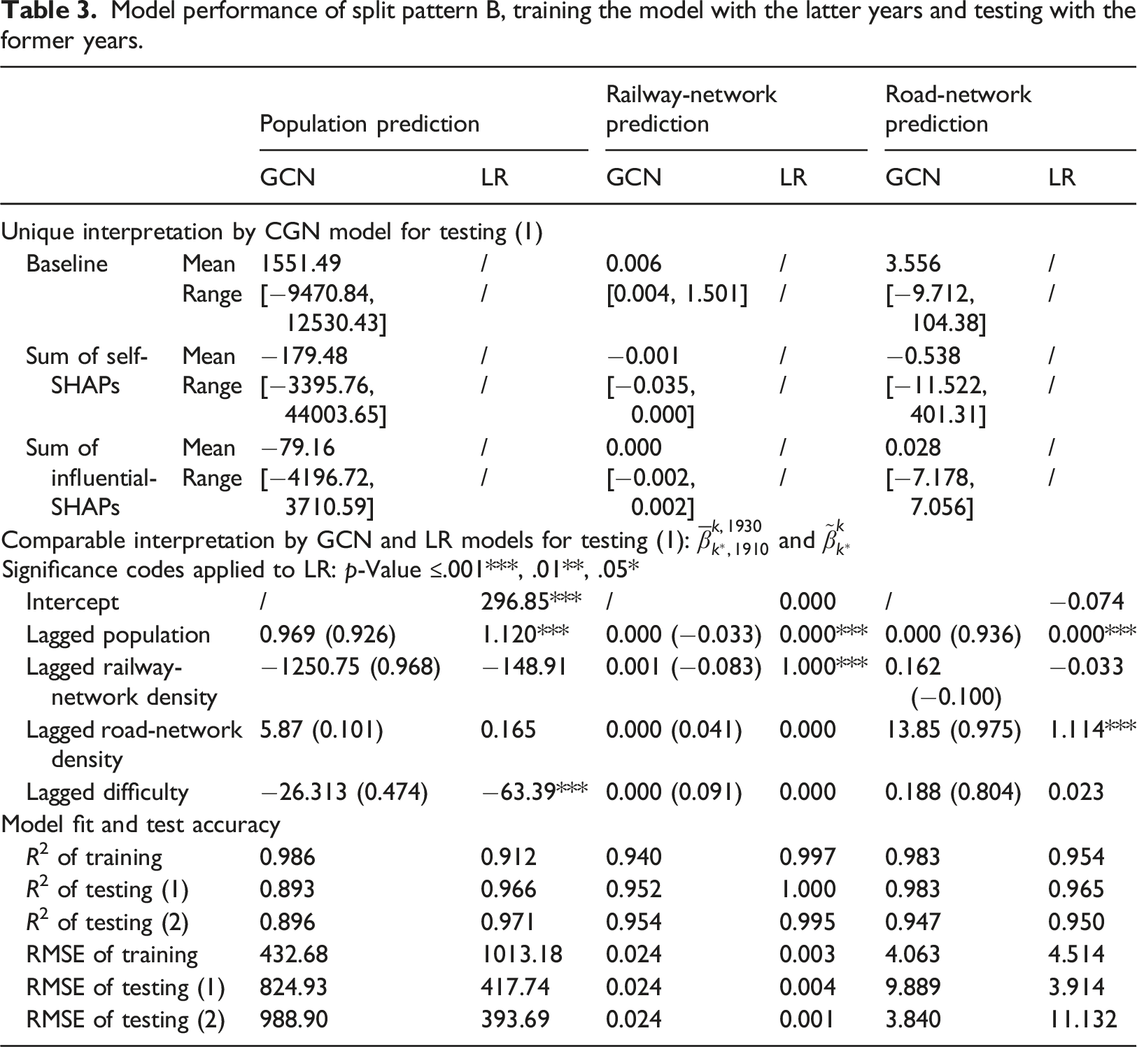
The comparison is divided into three parts. The first part, “Unique interpretation by CGN model,” shows the unique components that form the explanation by GCN on the regional development, which are the three terms of equation (6). We remind the reader that the baseline is node-specific, even if all node features are at their mean due to the asymmetric network topologies. (only in a fully connected network would the baseline be identical for each node). In general, the sum of self-SHAPs has a larger magnitude and a wider range than the sum of influential-SHAP as is shown in the tables. More specifically, the ratio between the absolute sum of self-SHAPs and the prediction value is, on average, 2.036, 0.353, and 2.531 for all nodes in the prediction of the population, railway-network density, and road-network density in 1990, respectively. The ratio between the absolute sum of influential-SHAPs and the prediction is 0.370, 0.073, and 0.952. Therefore, the lagged features of a node itself may predict the future features of the node to a considerable degree, which is confirmed by the equivalently good model fit and prediction accuracy achieved by the LR model using merely the lagged self-feature.

The second part compares the two sensitivity indicators $β_{i, k^{*}, t - 1}^{k, t}$ and ${\tilde{β}}_{k^{*}}^{k}$ , where we reiterate that one is node-specific and the other is not. Calculating the mean from all nodes is one way to make them comparable, but it does not provide us model fit information. Instead, we fit $ϕ_{x_{i, k^{*}, t - 1}}^{y_{i, k, t}}$ and $x_{i, k^{*}, t - 1} - {\bar{x}}_{k^{*}, t - 1}$ with a single linear regression model without an intercept. The coefficient is considered to be the general ${\bar{β}}_{k^{*}, t - 1}^{k, t}$ for all nodes, and R² is used to measure to which degree $β_{i, k^{*}, t - 1}^{k, t}$ can be node-independent. This R² is provided in the brackets below each ${\bar{β}}_{k^{*}, t - 1}^{k, t}$ of the GCN model. As an example, in the 1990 population prediction based on 1970 data, the average marginal contribution of the population ${\bar{β}}_{1,1970}^{1,1990}$ equals 0.511, and the R² of fitting $ϕ_{x_{i, 1,1970}}^{y_{i, 1,1990}}$ and $x_{i, 1,1970} - {\bar{x}}_{1,1970}$ into a single linear regression model without an intercept is 0.941. More specifically, the predicted population in 1990 of a municipality increases by 0.511 persons (the population unit) for every person living in the municipality in 1970. The high R² indicates that most municipalities follow this trend, which is also illustrated in Figure 3(a). The red crosses represent 2833 points coordinated in a 2-D space as $(x_{i, 1,1970} - {\bar{x}}_{1,1970}, ϕ_{x_{i, 1,1970}}^{y_{i, 1,1990}})$ , and they are roughly on the same line, meaning that the coefficients $β_{i \in [1,2833], 1,1970}^{1,1990}$ are highly similar.

Figure 3.

Marginal contribution of four self-features in the prediction of the population and the road network density: 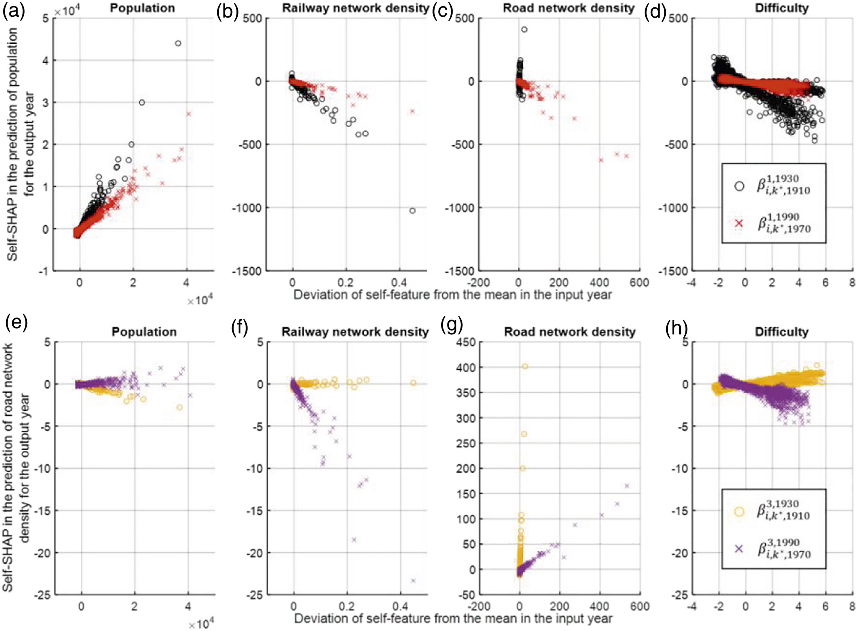$β_{i, k^{*}, t - 1}^{1, t}$ and $β_{i, k^{*}, t - 1}^{3, t}$ .

Although we cannot compare the magnitudes of ${\bar{β}}_{k^{*}, t - 1}^{k, t}$ and ${\tilde{β}}_{k^{*}}^{k}$ due to the difference between the definitions of GCN’s baseline and LR’s intercept, several conclusions can be drawn. Firstly, for some features, a global coefficient may be sufficient to describe the impact of the specific feature on future predictions. It can be seen that the R² values in brackets of the lagged population, railway-network, and road-network are all higher than 0.9 for the population prediction for both split patterns. The low R² values in brackets of the lagged difficulty in population prediction indicate the necessity to allow for node variability regarding its impact on the future population. The R² of the lagged difficulty GCN coefficient is reduced from 0.596 in split pattern A to 0.474 for B, showing that a model considering node-heterogeneity is necessary for the early years. We will expand on this point in “ Discussion on SHAP values ”. Secondly, we can observe that LR always estimates the future value of a specific feature to strongly rely on its previous status. ${\tilde{β}}_{k}^{k}$ is always estimated slightly larger than one and significant in the prediction of the $k^{th}$ feature. In the population prediction, the coefficient of lagged population is measured as 1.234 and 1.120 for split patterns A and B, respectively. The population did increase in general for every node, and a 20% increase imposed on the 1970 population can predict the 1990 population at an accurate level. In summary, “the rich remain rich.” The story told by GCN is fairly different; in 1990, only 51% of the amount higher than the mean population will carry over to the future, if all network attributes are identical. However, in 1910, 97% of the amount higher than the mean population will stay. The GCN results suggest that “the rich remain rich” is only true in the early years but that population shifts are far more possible in later years.

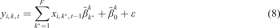
The third part of Table 3 reports goodness of model fit and test accuracy. R² and RMSE are used to evaluate the models for each prediction objective. The conclusion is that the prediction accuracy is fairly high by the LR models with only the lagged self-features. The testing R² of LR is always higher than 0.94, making it extremely difficult for the GCN to overperform. We find that the GCN is slightly overfitting the data in the training stage, and it fails to produce superior results, although the accuracy is acceptable. We conclude that the LR model (and other advanced models) is sufficient for providing good predictions as the population and network features 20 years ago are often similar to the predicted ones. The GCN model and the derived SHAP values, do, however, provide a rich source to interpret the results.

Discussion on SHAP values

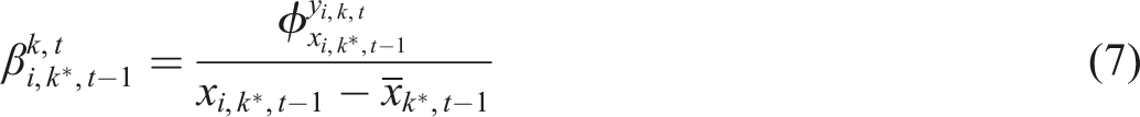
We now discuss the self-SHAPs obtained for each node. We recall equation (6) here. The numerator on the right side refers to the y-axis and the denominator to the x-axis of Figure (3). Each subplot of Figure (3) contains two sets of points denoting $β_{i, k^{*}, t - 1}^{k, t}$ , one for $β_{i, k^{*}, 1910}^{k, 1930}$ (circles) and the other for $β_{i, k^{*}, 1970}^{k, 1990}$ (crosses). The points on several subplots show obvious linear correlation, which is in line with those ${\bar{β}}_{k^{*}, t - 1}^{k, t}$ having high R² in brackets in “ Model performance and interpretation ”. We only show the results for population and road network density prediction, since we find that the railway-network density did not increase significantly in the studied century so that the results of the railway network are not explainable. The equivalent figure for rail-network density and the growth rate for all the development indicators can be found in the Supplemental Material for this section (Supplemental Figures S3 and S8).

Regarding the prediction of population, we can see in Figure 3(a) and (b) that the linear correlation, either positive or negative, was stronger in the early 20th century. It shows that in the late 20th century, the future population of a municipality was less determined by its own population and less decreased by its own railway-network density. This indicates an increasing tendency to move away from municipalities with a large population and a decreasing tendency to move away from municipalities that have a well-developed railway network. It is also noteworthy that the trend in the road-network density has changed drastically in the beginning and end of the 20th century. In the beginning, a high road-network density increased population sharply while it lost the attraction power to the population and even reduced the population in the late 20th century (Figure 3(c)). Taken together, the findings illustrate that residents are now more likely to move out of the municipalities with better accessibility as it becomes easier to commute from other places, and the main factor driving population to move out has shifted from the railway to the road network. We can hence quantify with our model the dynamics between the improvement in the transportation and the development of the suburbs. These findings cannot be obtained from the LR as the coefficient of the road network is positive in both the early and late 20th century cases.

The results obtained through our SHAP analysis regarding the impacts of difficulty on the population provide additional insights. Difficulty, which reflects topographical and economic constraints, tended to decrease the population in the future in two diverging ways in the early 20^th century as shown in Figure 3(d). Figure 4(a) then distinguishes these two trends of difficulty impacts by different colors with a threshold of −30, which is close to the average sensitivity of difficulty $β_{i, 4,1910}^{1,1930} = - 26.313$ . Figure 4(b) overlays the municipalities with correspondent colors on the railway network in 1910. It shows that the municipalities that lost population more easily due to difficulty were generally close to the railway stations. More specifically, the municipalities having better access to railway stations were more likely to lose population in 1930 given a same above-average difficulty in 1910, while they were more likely to gain population provided that the difficulty was lower than the average. Then in the late 20th century, the two diverging trends converge. This might result from the general improvement in the quality of life in less accessible regions and less need to move to well-connected places so that the population became less sensitive to difficulty, regardless of being close to a railway station or not. Hence, the analysis shows that there is a slowing tendency for the Swiss population to move away from the mountainous, difficult to access regions to the better connected and faster developed urban centers.

Figure 4.

Illustrating the municipalities having two different trends of 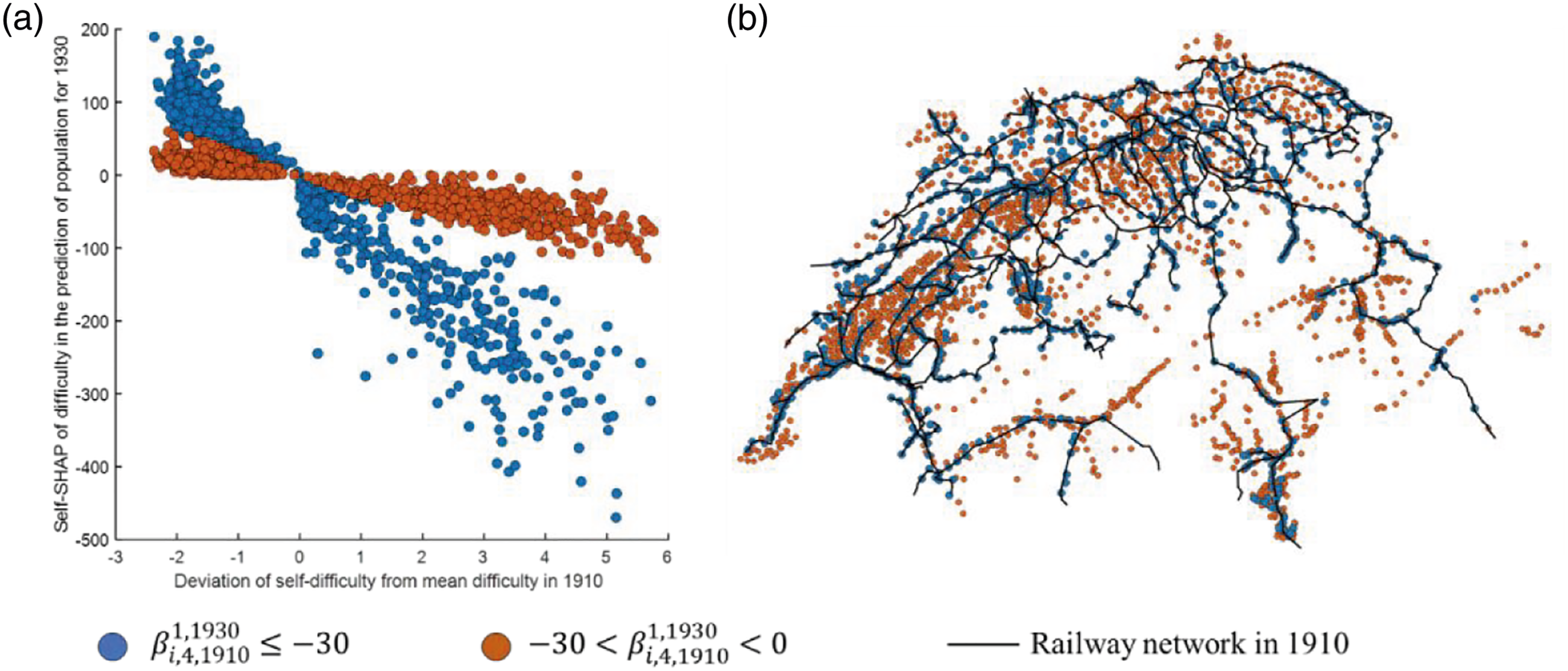$β_{i, k^{*}, 1910}^{1,1930}$ (Figure 3(d)) with the railway network in 1910.

In Supplemental Material Figure S9, we further show the correlation between the four feature values of the target node and the influential-SHAPs for population, rail-network, and road-network predictions. In general, we find that municipalities with smaller population size and worse transport infrastructure (lower network density) are more likely to be influenced by other municipalities.

Conclusion

Considering the importance of predicting complex regional development, as well as the lack of research focusing on long-term regional development, we have proposed a new methodology using deep learning with time series network data to predict long-term regional development. The proposed model explains the reciprocal relationship between population concentration and transport infrastructure development, considering transportation accessibility and road and railway network structures.

The graph-based model consists of several building blocks. The main module is a convolution of features across the node itself and neighboring nodes. This is supported by pooling and jumping modules to avoid having too many parameters and “over-smoothing,” that is averaging out all regional differences. Our assumption is that the regional developments trigger mutual development among the municipalities. In future research, alternative graph structures might also be considered. For example, in the case of centrally governed countries, this could suggest different graphs where each municipality is directly connected to the country’s capital. Moreover, we demonstrated that using the “GraphExplainer”, SHAP values can explain differences in influential factors for different nodes as well as different time periods. Even though simpler models such as linear regression can also provide a good overall fit, we show that the proposed approach can lead to additional insights by providing node and feature specific parameters.

Our results illustrate the changing population dynamics in Switzerland. Compared to several decades ago, predicting population growth or decline today requires a good understanding of the city’s connectedness. We demonstrate that higher connectivity can lead to population decline in surrounding municipalities. At the same time, low accessibility has led to population agglomeration in or near the larger municipalities. Whereas the suburbanization trend is increasing, the trend to move away from the mountainous areas is declining. Hence, one might use the approach presented here to also predict population distribution developments through further reduced distance deterrence as is expected by, for example, high-speed rail and autonomous vehicles. The SHAP values are amongst other powerful ones to illustrate the changing role of the Swiss geography on the population development. We illustrated and discussed the interplay between “geographic and economic difficulty,” rail accessibility, and population movements. Our analysis quantifies the declining role of transport accessibility, and we expect it to continue further given the increasing role of non-physical accessibility.

Supplemental Material

Supplemental Material—Explaining a century of Swiss regional development by deep learning and SHAP values

Supplemental Material for Explaining a century of Swiss regional development by deep learning and SHAP values by Youxi Lai, Wenzhe Sun, Jan-Dirk Schmöcker, Koji Fukuda, and Kay W Axhausen in Environment and Planning B: Urban Analytics and City Science

Footnotes

Declaration of conflicting interests

The author(s) declared no potential conflicts of interest with respect to the research, authorship, and/or publication of this article.

Funding

The author(s) disclosed receipt of the following financial support for the research, authorship, and/or publication of this article: Parts of this work were supported by JST SICORP Grant Number JPMJSC20C4, Japan.

ORCID iDs

Youxi Lai

Wenzhe Sun

Jan-Dirk Schmocker

Kay W Axhausen

Supplemental Material

Supplemental Material for this article is available online.

Author biographies

Youxi Lai is a former Bachelor and Master student of Kyoto University. She graduated from the International Course Program of Civil Engineering. Parts of this work formed the basis of her Master thesis in the Intelligent Transport Systems laboratory. She is now working at Hitachi, Ltd. Building System Business Unit.

Wenzhe Sun is a postdoctoral researcher in the Department of Urban Management at Kyoto University. His current research interests are learning the relationships between mobility, activity participation, and built environment, using crowdsourced big data and machine learning techniques. His recent work also focuses on explainable and interpretable deep learning.

Jan-Dirk Schmöcker is an Associate Professor in the Department of Urban Management at Kyoto University. His research focuses on the modelling of passenger decisions and broader public transport planning issues. Some of his recent work is also using various data for city tourism planning as well as regional planning scenarios.

Kouji Fukuda obtained his PhD from Tokyo University and is a Senior Research Follow in the Intelligent Information Research Department, Center for Technology Innovation - Advanced Artificial Intelligence at Hitachi. His main expertise is in machine learning and applying this to long-term simulations of urban and regional problems.

Kay Axhausen is Professor of transportation planning at the ETH Zurich. His recent work built on large scale GPS tracking and on a time-use survey app incorporating GPS tracking. The work is the basis for nationwide implementations of the agent-based simulation tool MATSim, co-developed by his group.

References

Akgüngür

Aldemir

Kustepeli

, et al. (2011) The effect of railway expansion on population in Turkey, 1856-2000. Journal of Interdisciplinary History 12(1): 135–157.

Axhausen

Hurni

(2005) Zeitkarten Schweiz. Zürich, Switzerland: IVT ETH Zürich. ETH research collection. DOI: 10.3929/ethz-a-005231332.

Bapaume

Côme

Roos

, et al. (2021) Image inpainting and deep learning to forecast short-term train loads. IEEE Access 9: 98506–98522.

Bairoch

(1976) Europe’s gross national product, 1800-1975. Journal of European Economic History 5(2): 273–340.

Chen

(2012) Agent-based modeling in urban and architectural research: a brief literature review. Frontiers of Architectural Research 1(2): 166–177.

Fuhrer

(2019) Modelling historical accessibility and its effects in space. Available at: https://www.research-collection.ethz.ch/handle/20.500.11850/406184

Fröhlich

Tschopp

Axhausen

(2006) Development of the accessibility of Swiss municpalities: 1950 to 2000. Raumforschung und Raumordnung 63(6): 385–399.

Kasraian

Maat

van Wee

(2016a) Development of rail infrastructure and its impact on urbanization in the Randstad, the Netherlands. Journal of Transport and Land Use 9(1): 151–170.

Fukuda

(2020) GraphExplainer. Unpublished. Hitachi seminar presentation.

10.

Kasraian

Maat

Stead

, et al. (2016b) Long-term impacts of transport infrastructure networks on land-use change: an international review of empirical studies. Transport Reviews 36(6): 772–792.

11.

Kingma

(2017) Adam: a method of stochastic optimization. Available at: https://arxiv.org/abs/1412.6980

12.

Lahoorpoor

Levinson

(2019) Trains, trams and terraces: population growth and network expansion in Sydney: 1861-1931. Working Paper. Available at: https://hdl.handle.net/2123/21350

13.

Lee

Rhee

(2020) DDP-GCN: multi-graph convolutional network for spatiotemporal traffic forecasting. arXiv:1905.12256. [Online]. Available: https://arxiv.org/abs/1905.12256

14.

Schmöcker

J-D

Qureshi

, et al. (2021) Historical transportation accessibility of Chinese Sui-Tang period and its socioeconomics influence. In: 14th International Conference of Eastern Asia Society for Transportation Studies (EASTS), Hiroshima, Japan, 12–15 September 2021.

15.

Gong

(2016) Urban Growth Models: Progress and Perspective. Berlin, Germany: Springer.

16.

Lundberg

Lee

S-I

(2017) A Unified Approach to Interpreting Model Predictions. Neural Information Processing Systems.

17.

Mimeur

Queyro

Banso

, et al. (2018) Revisting the structuring effect of transportation infrastructure: an empirical approach with the French railway network from 1860 to 1910. Historical Methods: A Journal of Quantitative and Interdisciplinary History 51(2): 65–81.

18.

Otgonbayar

BadarifuRanatunga

Onishi

, et al. (2018) Cellular automata modelling approach for urban growth. Reviews in Agricultural Science 6: 93–104.

19.

The World Bank (2020) https://data.worldbank.org/indicator/NYGNP.MKTP.CD?locations=CH

20.

Tschopp

Fröhlich

Axhausen

(2006) Accessibility development and its spatial impacts in Switzerland 1950–2000. In: 6th Swiss Transport Research Conference, Monte Verità, Ascona, 15–17 March 2006.

21.

Waddell

(2002) UrbanSim: modeling urban development for land use, transportation and environmental planning. Journal of the American Planning Association 68(3): 297–314.

22.

Wang

Yang

Ning

(2018) DeepSTCL: a deep spatio-temporal ConvLSTM for travel demand prediction. In: 2018 International Joint Conference on Neural Networks (IJCNN). Piscataway, NJ: IEEE, pp. 1–8.

23.

Sun

Hong

, et al. (2019) SocialGCN: An Efficient Graph Convolutional Network Based Model for Social Recommendation. Ithaca, NY: Cornell University. Available at: https://arxiv.org/abs/1811.02815

24.

Xie

Levinson

(2011) Evolving Transportation Networks. Berlin, Germany: Springer.

25.

Yin

Zhu

(2018) Spatio-Temporal Graph Convolutional Networks: A Deep Learning Framework for Traffic Forecasting. Ithaca, NY: Cornell University. Available at: https://arxiv.org/abs/1709.04875

Supplementary Material

Please find the following supplemental material available below.

For Open Access articles published under a Creative Commons License, all supplemental material carries the same license as the article it is associated with.

For non-Open Access articles published, all supplemental material carries a non-exclusive license, and permission requests for re-use of supplemental material or any part of supplemental material shall be sent directly to the copyright owner as specified in the copyright notice associated with the article.

0.00 MB

2.11 MB