Sage Journals: Discover world-class research

Abstract

This study provides a unique long-term investigation of regional travel demand that addresses several gaps in the existing longitudinal literature. Firstly, it investigates the development of travel demand in terms of both vehicle kilometres travelled (VKT) and passenger kilometres travelled (PKT), based on actual demand, congestion and equilibrium distances, using road and multi-modal transit networks in the Greater Toronto-Hamilton Area (GTHA). Secondly, it identifies influential travel demand determinants after testing an extensive set of variables including longitudinal gravity-based transport accessibility measures. Thirdly, it investigates to what extent the determinants’ influence changes over time and various locations within the study area, providing new insights into the temporal and intra-regional variations of travel demand and its determinants. The findings show that VKT and PKT have grown in absolute and per trip terms, mainly due to substantial population growth, especially in the suburban areas. Whilst average potential travel times by transit have decreased, they are substantially longer than auto travel times. Furthermore, travel demand determinants vary significantly across space by degrees of urbanity, especially for VKT. The findings call for area- and population segment-specific land use and transportation policies across the GTHA.

Keywords

Travel demand vehicle kilometres travelled passenger kilometres travelled longitudinal analysis the Greater Toronto-Hamilton Area

Introduction

The modelling and estimation of long-term travel demand is vital for sustainable planning, providing an understanding of the effects of urban transport system changes on travel behaviour and informing decision-making for transportation infrastructure investments. As theorised by the land use transport feedback cycle (Wegener and Fürst, 1999), investments in transportation infrastructure change locations’ accessibility. This leads to re-distribution of land uses, followed by changes in travel behaviour, which eventually induce the demand for new or improved transportation infrastructure. Travel behaviour is influenced not only by transport infrastructure and land use, but also by socio-economic factors, as well as spatial and mobility policies.

These factors are known to impact travel behaviour over time and at varying rates (Bertolini, 2012; Wegener and Fürst, 1999). Moreover, travel behaviour is affected by past travel patterns, changes over the life cycle and among generations, and could vary over time due to factors such as pervasiveness of habits, inertia and imperfect information (Dargay, 2007) or due to residential self-selection (Cao et al., 2007). Thus, travel behaviour, including the demand for travel, is dynamic in nature and evolves gradually – barring exceptions such as sudden reactions to gasoline price shocks.

The success of various travel demand management and transportation system investment policies hinges on knowing how the built environment and other determinants impact travel demand across different regions. As these impacts only become evident over time; they are unobservable in the cross-section (Su, 2010). There is, however a relative lack of longitudinal studies of built environment and travel behaviour (Zhong et al., 2020). Whilst the number of studies is increasing, the majority are still cross-sectional and aggregate in nature (Feng et al., 2017).

Figure 1S in the Supplementary Material provides an overview of peer reviewed journal articles that investigate the link between the various determinants longitudinally, that is using (pseudo-) panel, time-series and repeated cross-sectional data since the year 2000. The studies operationalise travel demand by, among other variables, vehicle kilometres travelled (VKT) for auto-based trips and passenger kilometres travelled (PKT) for transit-based trips. These are important indicators of the efficiency of land use and transportation planning which summarize various aspects of travel demand (number of trips, spatial trip distribution, travel modes and used routes) within a single measure (Miller and Ibrahim, 1998). Furthermore, they are convenient measures for multi-decade investigations as they can be rather consistently measured over long time periods. Due to our regional focus, micro-level studies such as studies of neighbourhood-level residential self-selection or focussing on single events (e.g. the travel demand consequence of a new rail line) are excluded.

Table 1 summarizes the significant factors contributing to VKT or PKT, as identified by longitudinal studies, categorized into three groups: the built environment, socio-economic and transportation factors. Here we discuss a number of significant factors per group and the rationales for their expected relationships with VKT and PKT. For a more detailed review of VKT/PKT determinants see the Literature Review section of the Supplementary Material.

Table 1.

Significant determinants of VKT and PKT identified by longitudinal literature.

Built Environment

Density and its proxies (e.g. distance of the household from the central business district (CBD))

Centrality (concentrations of population/employment)

Land use mix

Road layout

Socio-Economics

Age

Gender

Income (household or personal)

Car ownership

No. of workers in a household

No. of children in a household

Driving licences (per adult and dependent population)

Transportation

Road and transit supply and accessibility (proxied by length or density, possibly normalized by population size)

Congestion

Car purchase price

Driving costs (fuel price and fuel efficiency per mile)

Transit fare

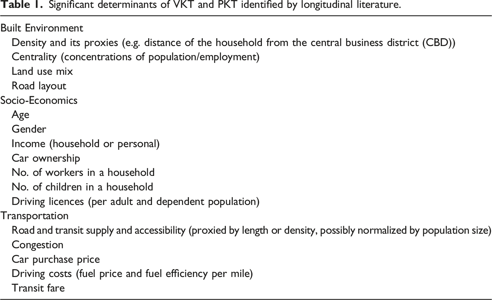
An important built environment factor is density. Higher density reduces the distance between activities and is argued to provide the critical mass needed for efficient transit service (Pushkar et al., 2000). It facilitates active transportation modes and transit as viable alternatives for auto, leading to higher PKT and lower VKT. Density also has an indirect effect: by reducing the distances between activities, it shortens the access and egress times to transit, thus encouraging its use (Limtanakool et al., 2006). A reverse relationship exists in low density sprawling suburbs where people are located farther from activity centres and depend on cars to reach them. Growing suburbanization is expected to result in increased VKT and reduced PKT.

Significant socio-economic factors include income, age and gender. Higher income is expected to increase the purchasing of cars and thus their greater use (Pushkar et al., 2000). Age is a recognized determinant of mode and distances travelled. Population aged 20–64 is reported to travel more by car and less by transit, as this age band corresponds with (peak) professional activity and presence of dependent children (He and Zhang, 2011).

Several studies have reported a general age-related decline in distances travelled among seniors, which is attributed to a decrease in their willingness and/or the ability to drive (Mercado and Páez, 2009; Schmöcker et al., 2005). On the other hand, Senior citizens are expected to keep their car-dependent lifestyle, which is a legacy of coming of age in sprawling auto-driven areas, and even possibly drive more (Figueroa et al., 2014; Hildebrand and Myrick, 2001). This corresponds to their increasing income and car availability and the desire to maintain their independent travel and mobility. The heterogeneity of seniors’ car use can be explained by various socio-economic, spatial structure and cohort characteristics (Figueroa et al., 2014; Kuhnimhof et al., 2013). For instance urban environments with higher population density (a proxy for transit access and short walking distance to destinations) and neighbourhoods with high commercial and residential mix are shown to be associated with seniors’ lower likelihood of driving and lower VKT (Hildebrand and Myrick, 2001; Kim and Ulfarsson, 2004; Mercado and Páez, 2009). Share of seniors is expected to be negatively correlated with PKT due to barriers for transit use for seniors such as inconvenient pedestrian access to transit stations and uncomfortable waiting areas (Babka et al., 2008). Furthermore, men are more likely to own and use private vehicles. However, this gap is observed to have closed in some developed countries possibly due to a trend increase in female labour participation and gender equality that has blurred the gender roles, coupled with a reduction in young males’ car travel (Kuhnimhof et al., 2012).

As for transportation related factors, higher supplies of road and transit or lower transit fares/gas prices, reduce the costs of travelling by these modes in terms of money and/or time. These increase accessibility by these modes, which in turn induces more demand for them. Transportation accessibility is investigated by a host of distance- or density-based variables measuring the supply of, or proximity to, road and transit. Few longitudinal studies, however, have operationalised the impact of accessibility over time through more sophisticated measures such as gravity-based potential accessibility indicators due to the lack of consistent land use and transportation data (an exception is Weis and Axhausen, 2009). These measures, which combine a positive function of destination size with an inverse function of travel cost to all destinations, are argued to better capture the impact of transportation accessibility on travel behaviour, as they combine both land use and transportation elements (Geurs and Van Wee, 2004; Weis and Axhausen, 2009). Finally, it is important to pay attention to the correlations between the above determinants (e.g. density, income and car ownership) and variations of their significance and sign over space.

It should be noted that, changes in social trends or technological and policy trends that have social consequences also influence travel demand (Zhao and Li, 2021). Several sources and trends of social change are observed by the (longitudinal) literature that have implications for travel demand. Firstly, shifts in lifestyles and attitudes and transportation preferences of various socio-economic groups has influenced travel demand over and above the classical ‘objective’ factors. For instance increasing concerns about health and obesity and environmental degradation are identified as reasons to drive less (Lucas and Jones, 2009). Furthermore, private vehicles are being perceived as less important as a status symbol by millennials, contributing to postponed/lower driving licence and private vehicle acquisition and less car use in this group (Delbosc and Currie, 2014). Such shifts in mobility patterns are further supported by the advances in the information communication technology (ICT) that have contributed to the rise of the internet society, a shift towards ICT-based activity patterns and making transportation alternatives more convenient (Van der Waard et al., 2013; Van Wee, 2015). Finally, a reduction in VKT may be due to increased international mobility (Van der Waard et al., 2013) and a switch to air travel (Millard-Ball and Schipper, 2011).

Overall, the existing literature suffers from several research gaps:

1. Multi-decade studies are few (Kasraian et al., 2018).

2. Motorized transportation (VKT) studies dominate, excluding the role of transit.

3. Few studies have investigated variations across regional sub-areas (Choi, 2018). Travel demand can vary significantly within and between sub-regions due to variations in their built environment, socio-economic characteristics and transportation accessibility levels. However, such differences could be masked at an aggregate level (Ke and McMullen, 2017).

4. Longitudinal studies have paid insufficient attention to the influential role of transportation accessibility in travel demand and transportation accessibility has mostly been measured with simple indicators, such as distance to transit stations or road density of an area.

In short, the literature has mainly overlooked the role of temporal and geographic locational effects in modelling travel demand (Pirotte and Madre, 2011; Thanos et al., 2018). Furthermore, longitudinal works of several decades on both car and transit travel demand, that model transport accessibility by more sophisticated indicators like potential accessibility and investigate the intra-regional differences of determinants, are very scarce.

This paper addresses the above gaps by (i) empirically investigating the development of travel demand in terms of both VKT and PKT over three decades within a large and fast-growing metropolitan region, (ii) using a comprehensive set of built environment, socio-economic and especially transport accessibility (including potential accessibility) determinants, whilst (iii) emphasizing variations in travel demand and its determinants over time and space.

It does so in three parts. Firstly, a comprehensive, multi-decade (1986–2016) database characterizing travel demand, land use, transportation system performance, etc., is constructed for the study region (Data). Secondly, the long-term trends in travel demand within the region are investigated to identify the spatial and temporal variability in travel demand that has occurred over the past 30 years (Trend analysis). Thirdly, the determinants of travel demand dynamics within the region are assessed using a panel econometric model (Methods and Model results). Finally, policy implications of the findings from this analysis are discussed in Summary of findings and policy implications.

Data

The study area, shown in Figure 1, is the GTHA. The GTHA population is 7.1 million with Toronto as the urban core having a population of 2.7 million (2016 Census). The GTHA is served by a multi-modal transportation system, consisting of an extensive road network and public transport systems ranging from buses, streetcars, bus rapid transit, light rail and subway to commuter buses and rail.

Figure 1.

The GTHA in 2016.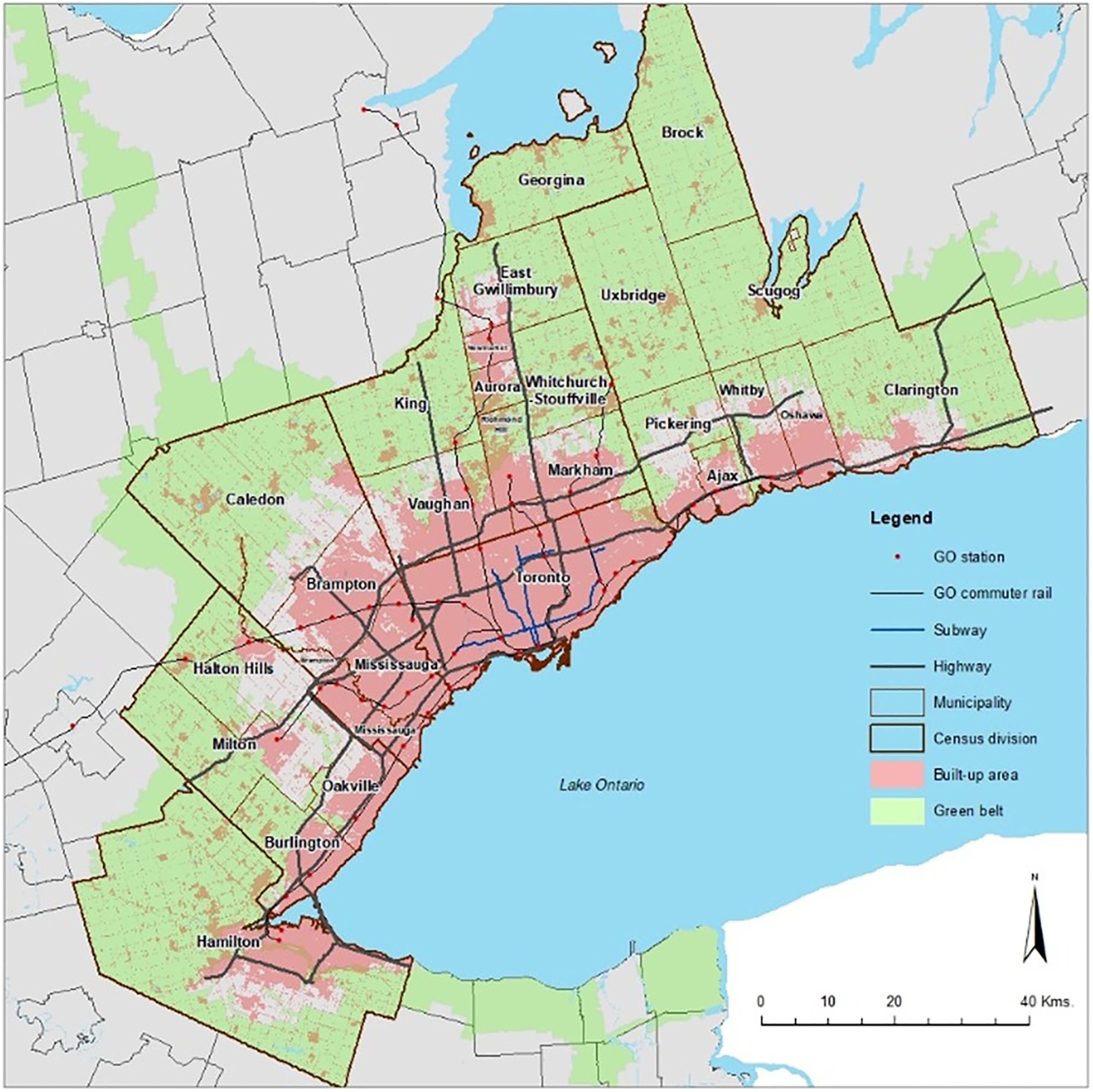

The GTHA is the most economically vibrant and dense contiguous urban area in Canada. It is the fastest-growing metropolitan region in Canada, with a population growth rate of 5.8% between 2011 and 2016 (2016 Census), and one of the fastest-growing regions in North America. This makes it an apt case-study for investigating long-term auto and transit travel demand patterns in relation to the expanding urban structure and changing demographics and accessibility levels over time. Total daily vehicle kilometres travelled (VKT) generated by trips originating in each GTHA zone were computed for a typical weekday (not a holiday) based on observed trips in the Transportation Tomorrow Survey (TTS) for seven time points (from 1986 to 2016 at five-year intervals). The TTS data is expanded using weight factors for each time period. The weighting is determined at both the person and household levels so that the weighted TTS sample matches census socio-economic distributions as best as possible (Malatest, 2018). Intrazonal trips are included in these calculations. The 2001 traffic zone system, consisting of 1716 zones was used for all calculations for all years. Similarly, total daily transit passenger kilometres travelled (PKT) were calculated for each origin zone for each year, again based on observed TTS transit trips. Intrazonal transit trips are virtually non-existent in the TTS data and so no attempt to compute intrazonal trip distances was made. The Construction of Dependent Variables section of the Supplementary Material provides full documentation of the methods used to construct the VKT and PKT variables.

The primary sources for the independent (explanatory) variables are the TTS and Census for travel-related and socio-economic data, respectively, from 1986 to 2016. Census data was collected for enumeration areas and converted to 2001 TAZ boundaries by areal weighted interpolation in ArcGIS, to be consistent in scale with TTS variables. All monetary values have been converted to constant 2016 Canadian dollars. The independent variables can be grouped into three categories:

1. Built environment indicators: TAZ-level variables for population density, job density, built-up area fraction, dwelling density, housing typology and tenure, road and transit line densities, self-containment ratio, effect of Greenbelt and degrees of urbanity.

2. Socio-economic indicators: population age distribution, number of households, household size, median and average household income, shelter costs for owned and rented dwellings, average value of dwelling, education levels, labour force characteristics, place of work status, employment type, industrial classifications of the employed population and household car ownership distribution.

3. Transportation indicators: Driving cost, actual and potential travel times by auto and time-based accessibility measures by auto and transit.

Detailed definitions of these variables and description of their construction are provided in the Construction of Independent Variables section of the Supplementary Material. Two variables, however, require some explanation here. Firstly, levels of urbanity vary in the GTHA, with Toronto and Hamilton being dense city cores, surrounded by sprawling suburbs and urban-rural fringe areas. Zonal trip-end (sum of trip origins and destinations for a given zone) densities (as observed in TTS for each survey year) over the study period are divided into 6 quantiles. Each TAZ is assigned to one of these 6 categories (henceforth abbreviated as ‘C’s) in increasing degrees of urbanity. These categories correspond with the ‘very rural’ (C1), ‘rural’ (C2), ‘in-between (mostly rural)’ (C3), ‘in-between (mostly urban)’ (C4), ‘urban’ (C5) and ‘very urban’ (C6) areas.

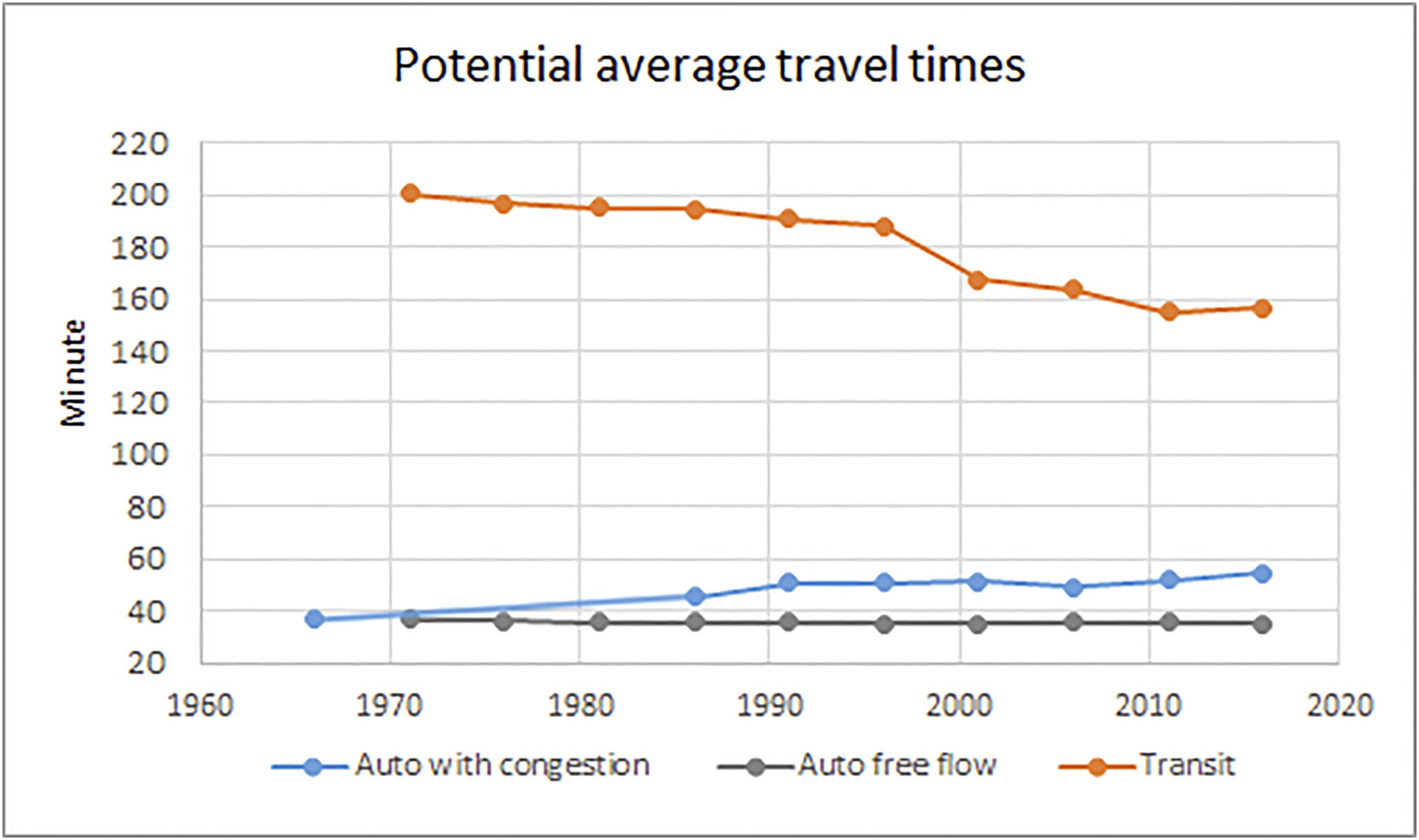
Secondly ‘potential average travel times’ by transit and car is simply the average travel time from a given origin zone to all destination zones within the GTHA, regardless of whether any trips are actually made to a given destination. This is a very abstract measure of a zone’s overall connectivity to all possible destinations in the region that captures the effects of road congestion and changes in road and transit supply over time. This average time is scaled by the population-weighted average for all zones to create a relative potential accessibility for each zone for both auto and transit.

Trend analysis

The evolution of rail transit and highway networks in the GTHA along with the growth of population are illustrated in Figure 2S in the Supplementary Material. It can be observed that both highway and rail networks expanded the most between 1976 and 1986 (Kasraian et al., 2020). Furthermore, cycles of increased growth in transportation infrastructure seem to follow population growth peaks. The economic slowdown of the early 90s is reflected in the reduced growth of both population and transportation infrastructure investments during the same period. Road and transit construction pick up again in the new millennium.

VKT and PKT have been growing in absolute and normalized per trip terms (Figure 2(a)–(b): over the past 30 years GTHA VKT and PKT have more than doubled. A closer look at TAZ-level PKT and VKT generation by degrees of urbanity (Figure 2(c)–(d)) reveals that travel demand varies significantly over space. The highest VKT growth belongs to the rural (but not very rural) areas. Conversely, the highest PKT generation and growth belong to the very urban areas, which include major population and job centres. Mean VKT and PKT per trip have also increased over the study period by 1.5 km and 4 km for auto and transit trips, respectively. So, over three decades, not only have VKT and PKT increased in absolute terms (mainly due to increasing population), but also longer distances are travelled by car and, specially, transit. Figure 3 compares potential average travel times from all TAZs to all TAZs over the GTHA road and transit networks over time. Potential average transit travel times have significantly decreased over the study period due to substantial improvements in transit supply. However, potential travel times by transit are still substantially longer than auto travel times. For instance in 2016, average potential transit travel times is still approx. three times higher than average potential auto travel times with congestion. On the other hand, potential average auto travel times show an increasing trend when congestion is accounted for. The dashed line indicates a linear interpolation between 1964 and 1986, given lack of data to compute congested auto travel times for the intermediate years (see the Construction of Independent Variables section of the Supplementary Material for details). Thus, despite improvements to the road network, auto travel times have increased, probably due to a combination of induced demand and growth in population.

Figure 2.

Trends in VKT and PKT. (a) total; (b) per trip; (c) and (d) total VKT and PKT per degree of urbanity.

Figure 3.

Trends in GTHA potential average travel times by auto (with congestion and free-flow) and transit.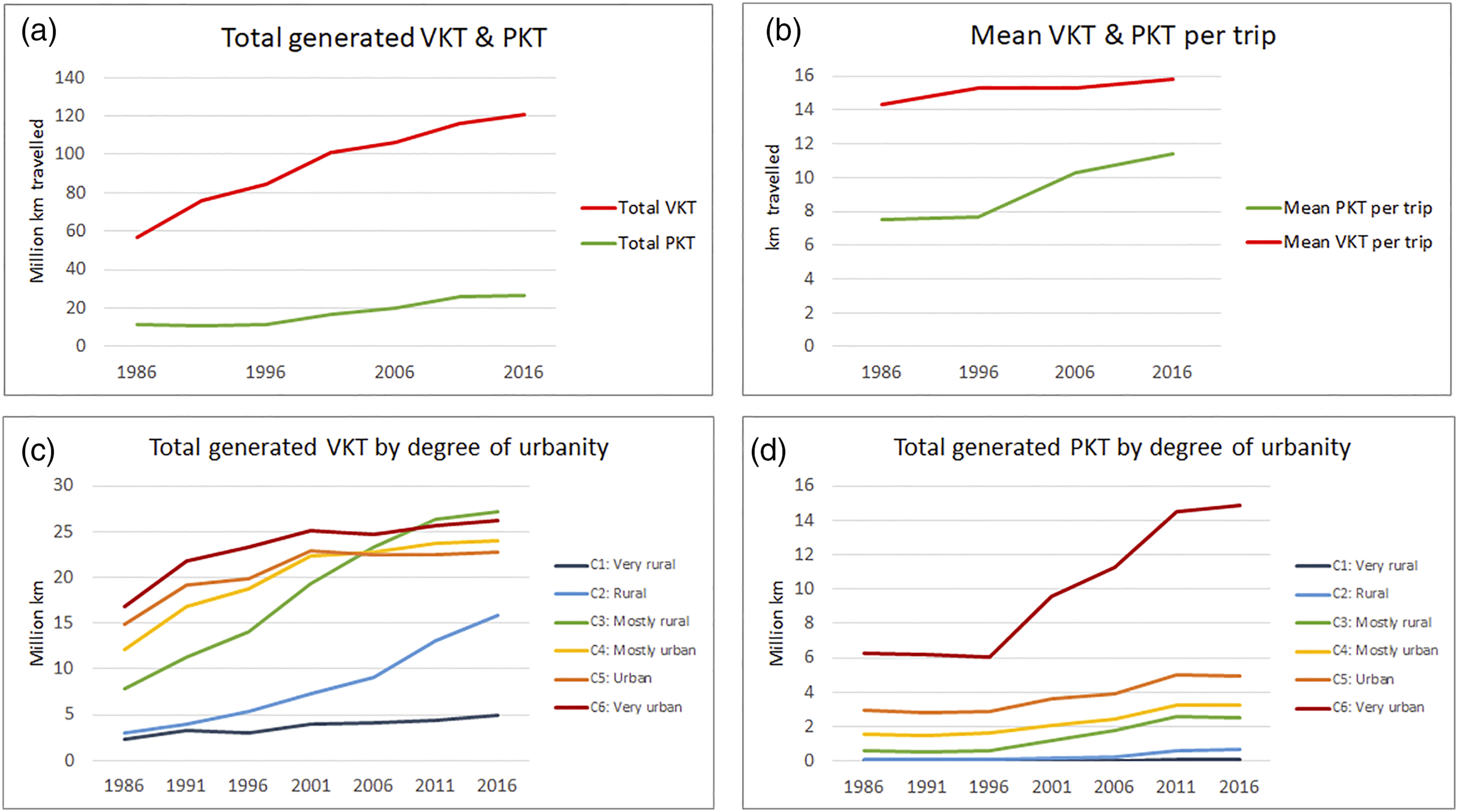

Methods

The analysis method should control for the fact that observations are nested within TAZs and model variations of travel demand over time and space. The most common methods applied to panel data are fixed-effects (FE) and random effects (RE) estimations.

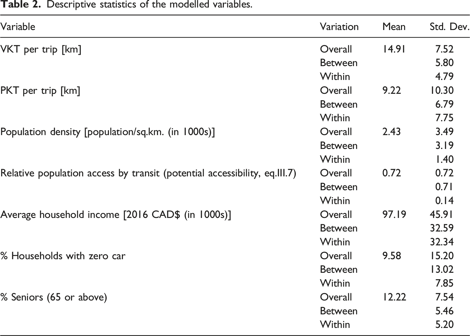
Here, the differences within TAZs over time are much less than the differences between TAZs over space. This is observable in the existence of greater between-unit standard deviations (or cross-sectional variation) compared to within-unit standard deviations (or time-series variation) for the majority of the investigated variables (Table 2).

Table 2.

Descriptive statistics of the modelled variables.

Variable	Variation	Mean	Std. Dev.
VKT per trip [km]	Overall	14.91	7.52
	Between		5.80
	Within		4.79
PKT per trip [km]	Overall	9.22	10.30
	Between		6.79
	Within		7.75
Population density [population/sq.km. (in 1000s)]	Overall	2.43	3.49
	Between		3.19
	Within		1.40
Relative population access by transit (potential accessibility, eq.III.7)	Overall	0.72	0.72
	Between		0.71
	Within		0.14
Average household income [2016 CAD$ (in 1000s)]	Overall	97.19	45.91
	Between		32.59
	Within		32.34
% Households with zero car	Overall	9.58	15.20
	Between		13.02
	Within		7.85
% Seniors (65 or above)	Overall	12.22	7.54
	Between		5.46
	Within		5.20

FE is a within estimator, as it measures the deviation from the mean within each panel unit over time. Thus, it is not able to capture the major between-unit variation in the dataset. As a result, a RE model was applied which captures both between-unit and within-unit variations. This model assumes exogeneity between the regressors and the unobserved heterogeneity at the TAZ-level. RE accounts for the data’s hierarchical structure with its multi-level structure by partitioning the unexplained residual variance into higher level (TAZs) and lower levels (observations). RE models are applied to both data with place-based hierarchies (like individuals nested within neighbourhoods) and temporal hierarchies (like panel data and time-series cross-sectional data) (Bell and Jones, 2014). Longitudinal studies with (pseudo-) panel data with temporal hierarchies have used RE to model travel behaviour indicators such as commuting times (Parent and LeSage, 2010), household car ownership (Nolan, 2010), passenger miles travelled and transit operation costs (Guerra and Cervero, 2011), and weekly kilometres travelled (Kuhnimhof et al., 2012).

VKT and PKT in TAZ $i$ at time $t$ are estimated by its built environment, socio-economic and transportation characteristics. The choice of a suitable subset of variables, which best explains variations in VKT and PKT, was based on a systematic process. Firstly, variables with high correlation with the dependent variables were identified. These variables (i.e. population density, potential transit accessibility and car ownership) conformed to the influential variables reported in the literature and showed expected signs. Secondly, multivariate models were tested where different combinations of independent variables were estimated to model a single outcome (VKT or PKT). These models showed a robust behaviour in terms of sign and significance. Thirdly, other potentially influential variables were added to the main variables and tested. As a result, two additional significant variables (i.e. income and percentage of seniors) were identified which had the expected signs and improved the model performance. According to the literature and theory presented in the Introduction section, we expect the built environment factor population density, to be negatively and positively correlated with VKT and PKT, respectively, as higher density could reduce distance between activities and support quality public transportation. Regarding socio-economic factors, having the means to purchase a car (higher income) and its availability (less households with zero cars) are expected to stimulate car use over transit, resulting in higher VKT and lower PKT. Furthermore, a higher share of seniors is expected to correspond with lower VKT and PKT in general, regarding the group’s reduced capabilities and professional activity and the existing barriers for transit use for seniors. However, we expect to observe spatial heterogeneity in seniors’ VKT across the region. Particularly, car-dependent rural areas are expected to reinforce the car use of seniors who strive to maintain their independent mobility in the absence of opportunities for walking and transit use.

As for the influence of transport factors, higher potential accessibility by transit is expected to reduce its cost, rendering it a viable option to compete with car in the face of rising congestion and car use restrictions, thus promote higher PKT and lower VKT. In short, the final choice of variables was based on including significant variables with expected signs as hypothesized by theory, whilst controlling for multicollinearity (between pairs of variables as well as the models’ mean collinearity indicated by the variance inflation factor (VIF)), and assessing various model performance statistics.

The models are estimated by the xtreg, re command in Stata, which applies a GLS random effects estimator. Since the RE estimator is a weighted average of between and within estimators, three R²s are reported for goodness of fit. The within-R² indicates the variance within the panel units accounted for by the model accounts (TAZs in this case), and is known as time-series variance. The between-R² shows the variance between the panel units accounted for by the model and is known as the cross-sectional variance. The overall-R² is a weighted average of the within- and between-R²s.

Finally, independent variables were interacted once with years and once with the degrees of urbanity to examine the variations in their effects over time and space. The introduction of interaction terms, specifically in the case of degrees of urbanity, resulted in some variables changing signs or significance in specific areas. The significance and sign of the interaction terms’ coefficients provide empirical evidence on the specific behaviour of travel demand determinants in the GTHA over time and across different degrees of urbanity.

The same procedure was repeated for choosing the most suitable functional form for the models, including, linear, semi-log and log-log formulations. All continuous independent variables are log-transformed. This reduces the risk of heteroscedasticity (Greene, 2003). For the VKT model, a linear-log functional form was chosen, where VKT experiences diminishing marginal returns as independent variables increase. This functional form accounts for saturation, where the increasing effects of various independent variables on VKT diminish. The PKT models had a significantly better fit with a double-log function, where a constant elasticity is assumed for all variables. Log-linear and double-log functional forms have both been extensively used for both car and transit travel demand analyses.

The performance of different indicators was tested during the procedure for selecting the final subset of independent variables. Population density is the only significant built environment indicator included in the models from a host of tested built environment variables including dwelling density, housing typology and tenure and self-containment ratio (See section III.1. ‘Built environment indicators’ of the Supplementary Material). Furthermore, spatial variations in the determinants are represented by interactions with the degrees of urbanity as proxies for types of built environment in the models. Regarding transport indicators, interestingly, models with potential accessibility variables outperform those with simpler travel time, (straight and network) distance to transit stations/highway exits and transit line density indicators. Furthermore, relative potential access to population by transit (hereafter transit access) has a higher performance for both VKT and PKT models than its auto-based counterpart. Employment access variables were also tested and were found to be highly correlated with population access and to perform similarly. Hence, this paper focuses on the results using population accessibility. The final panel dataset used to estimate the models presented herein consists of 6864 observations based on 1716 TAZs observed every decade (1986, 1996, 2006 and 2016).

The final models for VKT and PKT at TAZ $i$ at time $t$ are

V K T_{i}^{t} = β_{0} + β_{1} \ln {(p o p d e n s i t y)}_{i}^{t} + β_{2} \ln {(a c c e s s b y t r a n s i t)}_{i}^{t} + β_{3} \ln {(a v g . h h i n c o m e)}_{i}^{t} + β_{4} \ln {(% h o u s e h o l d s w i t h n o c a r)}_{i}^{t} + β_{5} \ln {(% s e n i o r s)}_{i}^{t} + β_{6}^{t} Y E A R^{t} + μ_{i} + ϵ_{i}^{t}

(1)

ln (P K T_{i}^{t}) = β_{0} + β_{1} ln {(p o p d e n s i t y)}_{i}^{t} + β_{2} ln {(a c c e s s b y t r a n s i t)}_{i}^{t} + β_{3} ln {(a v g . h h i n c o m e)}_{i}^{t} + β_{4} ln {(% h o u s e h o l d s w i t h n o c a r)}_{i}^{t} + β_{5} ln {(% s e n i o r s)}_{i}^{t} + β_{6}^{t} Y E A R^{t} + μ_{i} + ϵ_{i}^{t}

(2)

where

μ_{i}

accounts for all the time-invariant unobserved attributes for TAZ

i

. It is treated as a random term that is independently and identically normally distributed with zero mean and variance

σ_{μ}^{2}

β_{6}^{t}

captures the time-specific effects through year dummies

Y E A R^{t}

ϵ_{i}^{t}

, is the time-varying random error term, assumed to be an independently and identically distributed normal error term for i and t with zero mean and variance

σ^{2}

Model results

Two models were estimated for each travel demand indicator (PKT and VKT). The first interacted independent variables with the observation year (i.e. model parameters varied by year). These models generally show non-significant interaction coefficients and are not presented. In other words, the model parameters have remained relatively stable over time. In the second set of models, independent variables were interacted with the degree of urbanity at each point in space. These models with location interactions show interesting results and higher overall performance. These are discussed below.

Table 3 reports the parameter estimates for each explanatory variable for the base category, that is very rural areas (C1). The results show that population density and transit access are significantly and negatively related to VKT for very rural (C1) areas. Conversely, average household income, the share of seniors and the location of the TAZ existing inside the Greenbelt demonstrate a positive relationship in these areas.

Table 3.

VKT and PKT per trip estimation 1986–2016, random effects model with location interactions.

	VKT/trip	ln(PKT/trip)
Main effects at very rural areas (C1)
Population density (ln)	−0.616*	−0.050
Relative population access by transit (ln)	−1.354***	0.015
Average household income (ln)	0.574**	−0.001
% Households with zero car (ln)	0.008	0.117**
% Seniors (65 or above) (ln)	1.694***	−0.182*
Greenbelt	0.981*	−0.113
Interactions with degrees of urbanity
Population density*urbanity
C2	0.097	0.507***
C3	−0.256	0.432***
C4	−0.343	0.181
C5	−0.562	0.169
C6	0.732*	0.049
Relative population access by transit*urbanity
C2	0.565*	0.740***
C3	0.721*	1.241***
C4	1.514***	0.688***
C5	1.699***	0.350**
C6	3.023***	0.187*
Average household income*urbanity
C2	−0.006	0.029
C3	−0.333	−0.11
C4	−0.318	0.014
C5	−0.776***	−0.026
C6	−0.536*	−0.052*
% Households with zero car*urbanity
C2	−0.248	0.082
C3	−0.247*	−0.031
C4	−0.284*	−0.035
C5	−0.232	−0.138**
C6	−0.303*	−0.134**
% seniors*urbanity
C2	−1.632**	0.198
C3	−1.894***	0.011
C4	−2.246***	0.018
C5	−2.451***	−0.018
C6	−2.642***	0.148
1986 base year
1996	1.057***	0.176**
2006	1.648***	0.724***
2016	2.481***	0.886***
Base level of urbanity: Very rural (C1)
C2	4.114	1.002
C3	9.896**	4.648***
C4	10.917**	4.368***
C5	18.194***	4.890***
C6	6.538*	5.686***
Observations	6864	6864
$ρ$	0.18	0.14
R²_within	0.05	0.23
R²_between	0.58	0.81
R²_overall	0.36	0.63

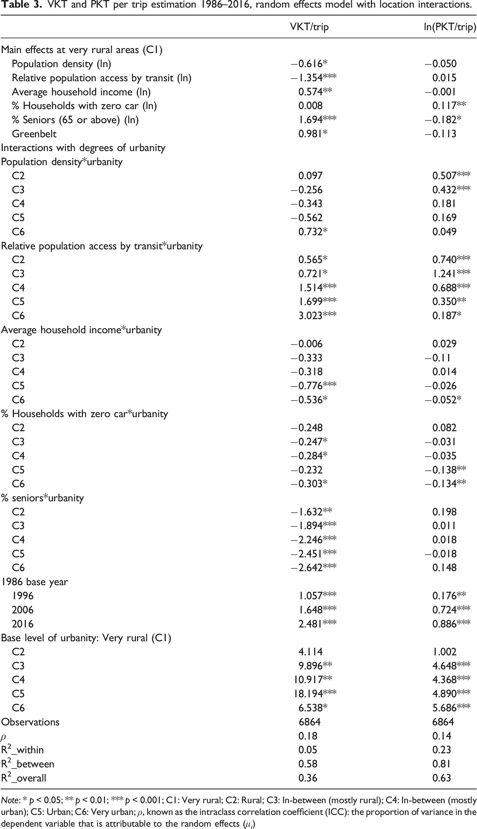
Note: * p < 0.05; ** p < 0.01; *** p < 0.001; C1: Very rural; C2: Rural; C3: In-between (mostly rural); C4: In-between (mostly urban); C5: Urban; C6: Very urban; $ρ$ , known as the intraclass correlation coefficient (ICC): the proportion of variance in the dependent variable that is attributable to the random effects ( $μ_{i}$ )

Interactions of independent variables with each urban category capture the difference in parameter values relative to the base category. Interestingly, the relations between population density and transit access with VKT reverse in very urban areas (C6) (Figure 4(a)–(b)). This seemingly counterintuitive result is because the very urban areas include major job centres. Whilst these areas have high transit access, they still attract substantial labour force from outer suburbs who commute by car, contributing to their high evening-peak VKT. The very urban areas are also CBDs with high population densities and intensity of land use mix, which may be responsible for the increased travel demand. The share of seniors, however, behaves conversely. As expected, seniors have the highest contribution to VKT in the very rural areas (C1). As the degree of urbanity rises however, seniors’ VKT decreases more and more (Figure 4(c)). This is probably due to a combination of shorter distances between activities and the feasibility of transit use and walking for the seniors in non-rural areas (C3-6).

Figure 4.

(a–d): Significant coefficients of VKT determinants (x-axis) by degree of urbanity; (e, f): Significant coefficients of PKT determinants (x-axis) by degree of urbanity.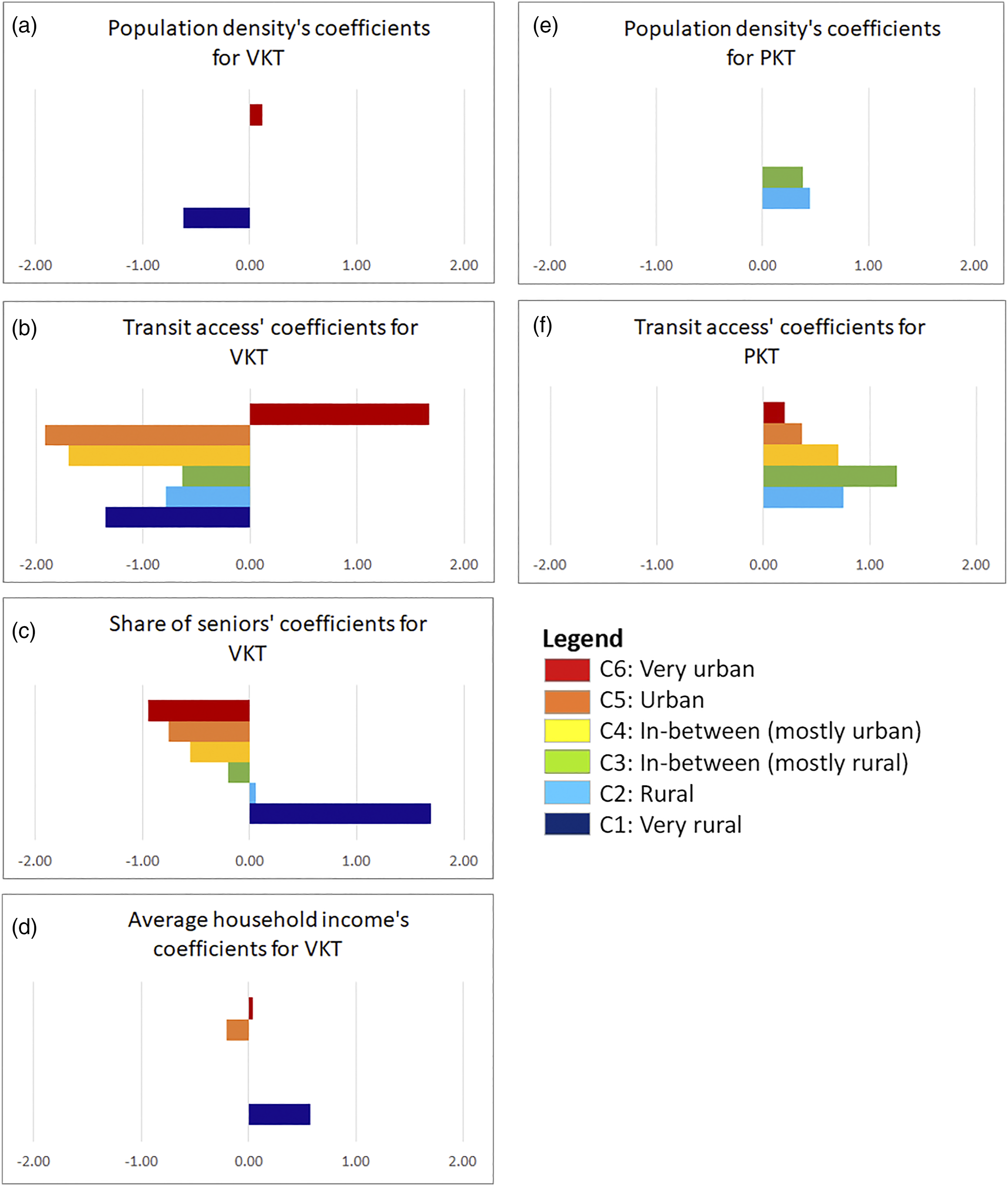

The contribution of income to VKT has the highest positive effect in very rural areas (C1) (Figure 4(d)), which means those who can afford automobile costs, prefer a car-dependent lifestyle. However, this relationship weakens and reverses in the urban areas (C5). This reflects the low VKT of relatively wealthy residents of city centres with nearby activity destinations. The very urban category (C6), which contains major job centres, does not show a substantial relationship between VKT and the household income of its residents. This is likely because of the commuting direction is generally from the suburbs and more rural areas to the centres in very urban areas. Thus, the VKT in the very rural areas consists of a substantial amount of home-based VKT which has a higher correlation with the household income of the residents in these areas. On the other hand, the VKT of the very urban areas is a combination of both its residents’ home-based VKT and the rural commuters’ work-based VKT, thus it does not show a substantial relationship with the residents’ household income.

The negative relationship between VKT and the share of households with no cars is generally present in the non-rural areas (C3-4 and C6), which have higher disincentives (congestion and parking costs) for car ownership and use. The majority of TAZs within the Greenbelt are very rural. Hence, the interaction effects of Greenbelt dummy with the higher degrees of urbanity are not significant and excluded.

As for PKT, the two significant variables at the very rural level are the share of households with zero cars and the share of seniors, which, as expected, are related to higher and lower PKT, respectively.

The role of population density is significant in the rural areas and the mostly rural in-between areas (C2-3) (Figure 4(e)). This is however not the case for the very rural areas (C1), which for the most part are large undeveloped tracts of land in the outer GTHA ring with a population density of less than 500 people per square kilometre.

The role of transit access is not significant only in the very rural areas (C1) where transit service is generally lacking and provides poor access to population centres. Moving along the very rural to very urban spectrum, the impact of transit access on PKT increases up to the medium-level degree of urbanity (C3), after which it weakens whilst remaining positive (Figure 4(f)). In other words, as the location becomes increasingly urban, the positive effect of transit access weakens. This could be due to a saturation effect of transit access following diminishing returns. This observation is in line with findings on the non-linear relationship between densification and transportation emissions generation due to VKT or congestion-related low travel speeds. It is reported that the strong negative relationship between characteristics of compact and dense land development, such as transit accessibility, and transportation emissions (proxy for VKT) weakens with increasing population density. This relationship may possibly become non-significant or reverse, after reaching a certain level of densification (Hong, 2017).

In very rural areas (C1) not owning a car has a significant and positive impact on PKT. Here, captive transit riders have to use transit to perform their daily activities. These activities are likely to be located in denser areas further away and/or dispersed across space, resulting in increased PKT. This relationship reverses in the urban categories (C5 and C6) but the effect is very weak and negligible.

The dummy year coefficients (relative to the 1986 base) indicate that both VKT and PKT have increased over time, especially for the PKT per trip between 1996 and 2006 (also reflected in Figure 2(b)). All things equal, PKT and VKT generally rise with the level of urbanity.

The overall-R²s show that the models explain nearly 36% and 63% of the overall variances in VKT and PKT. The between-R²s (i.e. the explained cross-sectional variance), are 58% and 81% for VKT and PKT, respectively. These are higher than the within-R²s, that indicate the time-series variance within TAZs over time accounted for by the model. This corresponds to the presence of generally higher between-rather than within-variation in the dataset (Table 2). More variance over time is explained for PKT, whose demand experiences a higher change during the study period compared to that of VKT (Figure 2(a)–(b)).

Summary of findings and policy implications

This study provides a unique longitudinal investigation that addresses several gaps in the literature. Firstly, it investigates regional travel demand evolution in terms of both VKT and PKT in one of the fastest-growing regions in North America over three decades. The VKT and PKT are calculated in detail based on TAZ-level actual 24-h demand and congestion-based equilibrium distances, using each time point’s road and multi-modal transit networks. Secondly, it identifies influential travel demand determinants after testing a comprehensive set of built environment, socio-economic and transport accessibility variables. Importantly, the role of potential accessibility is investigated, a useful indicator rarely used in long-term investigations due to lack of (consistent) data on land use and transportation. Thirdly, it investigates changes in determinants’ influence over time and locations within the study area, providing new insights into the temporal and intra-regional variations of travel demand and its determinants. To do so, it applies random effects models with interactions with time and degrees of urbanity to a panel dataset of 6864 observations.

The findings show that over three decades there has been a substantial development in GTHA transit infrastructure and a reduction of potential average travel times needed to reach various destinations by transit. Despite improvements to the road network, potential auto travel times have increased, probably due to a combination of induced demand and growth in population. Whilst average potential travel times by transit have decreased and average potential auto travel times have increased, the first is still substantially longer than the latter.

PKT and VKT have grown in absolute and per trip terms. Total PKT and VKT have both more than doubled. Nevertheless, PKT growth (especially total PKT), is substantially less than VKT growth. Highest VKT growth has taken place in the rural (C2) and in-between (mostly rural) areas (C3). Highest PKT generation and growth have happened in the very urban areas. Furthermore, GTHA residents are travelling longer distances by vehicles (1.5 km) and transit (4 km) on average, compared to 1971.

Approximately 60% and 80% of the variations in PKT and VKT between the GTHA TAZs can be explained by population density, transit access, household income, share of households with zero cars and the population share of seniors. Potential accessibility variables (namely, relative access to population by transit and auto) are found to outperform more simple indicators (such as distance to transit/road and transit line density) in explaining travel demand.

Interestingly, interactions of the independent variables with time were found to be generally not significant. The absence of time trends in the determinants shows that the effects of influential VKT and PKT determinants have been fairly stable over time. In other words, our determinants can reasonably predict the travel demand in the region, without much change in their influence over time. This is consistent with the findings of Ozonder and Miller (2021) in which trip generation rates for the region are found to be very stable over the 1996–2016 time period.

The increase in total VKT and PKT can be mainly attributed to a significant rise in the region’s population and its continuous suburbanization. Between 1986 and 2016, the population of GTHA and the foot print of its built-up area have increased with nearly 80% (Statistics Canada, 1986–2016) and 85% (Kasraian et al., 2020), respectively. Demographic change is a main determinant of travel demand that influences it by changing land use (Metz, 2012). In other words, where the added population lives and works determines how the population increase affects travel demand. A major part of the increasing population in the past decades have been channelled to in the suburban areas of GTHA due to the existing limits for development and high land value in Toronto’s inner city. On the other hand, the region’s monocentric structure requires long travel distances between these areas and working opportunities and amenities mainly focused in Toronto downtown.

The growth of VKT in the suburban areas is evident in our analysis (Figure 2(c)). Our findings also show that the highest PKT growth is taking place in the very urban areas such as the Toronto downtown, despite transit access showing a weakening influence in these areas. This coupled with the finding that average transit trip lengths have increased by 4 kms in the GTHA, indicates that a substantial working population from suburban areas is commuting via transit to central job locations, generating high evening PKT.

The presence of significant variations in the contribution of determinants on travel demand across degrees of urbanity is an important finding. The extremities of the rural to urban spectrum demonstrate unique behaviours, especially in the case of VKT determinants. Population density, access by transit, household income and the share of seniors have the highest explanatory power in predicting VKT in the very rural areas (C1) which are for the most part undeveloped and sparsely populated. The impact of population density, income and transit availability is in line with the findings of previous researchers (Ke and McMullen (2017), Oregon; Choi (2018), Calgary). In the very urban category (C6), the relationships of these variables with VKT are reversed. This is because very urban areas include major job centres and whilst they benefit from high transit access, they also attract car work-commuters from the outer suburbs.

Another important finding is that travel demand in terms of trip lengths has steadily increased in the GTHA. Despite both road and rail network growth, potential auto travel times have increased, whereas potential transit travel times have reduced. This shows the long-term positive outcomes of investing in transit infrastructure in the region. However, potential transit travel times are still on average substantially higher than their car-based counterparts, making transit an unviable alternative to driving in many areas. GTHA residents travelling longer distances suggests outward urban expansion and calls for an assessment of urban transport and land use planning policies affecting future travel behaviour.

The variation of travel demand by degrees of urbanity emphasizes the limits of one-size-fits-all travel demand management policies. There is a critical need to develop area-specific land use and transportation policies within a metropolitan region. For example the results indicate that a substantial working population from suburban areas is commuting via transit to central job locations, generating high evening PKT and increasingly longer transit trip lengths. This trend needs to be monitored closely, to cater to the transit demand of suburban commuters, as well as evaluate the need for greater decentralization of employment centres.

The transport policies also need to target specific population segments within regions. For instance seniors are shown to be more car-dependent in the rural and very rural areas (C1-2). Here, investments in infrastructure for active transportation which is safe for the elderly and alternative transportation such as on-demand paratransit could be beneficial. Similarly, specific policies for car-free households to encourage/support multi-modal transit and active modes, and provide alternative travel options like shared mobility services, are critical for preventing these households (especially in the very rural areas) from purchasing a car.

More effective VKT reduction policies are needed in the rural (outer suburbs) and mostly rural in-between areas (C2-3), which are shown to have experienced the highest VKT growth in the last decades. Fortunately, the findings also indicate that densification strategies and investment in transit access are likely to contribute the most in these areas, which are far from population and accessibility saturation levels.

An interesting finding is that very urban areas still generate very high VKT despite their high population density and their high accessibility by transit. This calls for stronger demand management policies to limit cars entering employment centres and facilitating the modal shift to transit for commuters. This can be achieved by increasing the cost of parking, which has been shown to be effective in central Toronto (Hatzopoulou and Miller, 2008), or implementing congestion pricing like London, Singapore, and more recently, New York. Another policy can be decentralising employment from the central areas to regional (sub-) centres whilst improving transit accessibility to these centres (Sim et al., 2001), especially since introducing or reinforcing transit connections to activity centres is found to encourage transit-led developments in the region (Kasraian et al., 2020).

It is important to note two main caveats of this study. Firstly, this is a meso-level study that aggregates all generated trips at the TAZ-level. Whilst this is a useful indicator to distinguish zones with high VKT/PKT, their time trends, and eventually potential measures to facilitate high travel demand, it is an aggregate measure that does not differentiate between trip purposes. Trips with different purposes have different impacts on transport infrastructure and eventually demand different transport management policies (Zhao and Li, 2021). Thus, future studies could differentiate between the trip purpose (e.g. home-based work/non-work trips) and investigate travel demand determinants related to the location of work and other purposes in addition to that of residential location. In addition, future work might investigate spatial-temporal variations in VKT by households based on their total daily tours and residential locations. Secondly, the unexplained variations in our models could be due to missing influential factors such as work location characteristics (e.g. disincentives for car use like parking price), transit fare prices and indicators that capture suburbanization. Furthermore, it is argued that the ‘subjective’ determinants of travel demand that include lifestyle elements such as personal attitudes, aims and location preferences are increasingly becoming important in developed countries (Ohnmacht et al., 2009; Scheiner, 2010). In the absence of longitudinal subjective data, this study has investigated the objective determinants of travel demand. Future studies are recommended to also investigate subjective lifestyle-related characteristics and their trend changes to shed light on variation in travel demand unexplained by classical objective indicators.

Despite these caveats, the paper’s methodology, the use of longitudinal gravity-based accessibility indicators, and interacting travel demand determinants with different degrees of urbanity (proxied by trip density) can be useful for future longitudinal studies of travel demand. Moreover, these findings can be relevant for other comparable fast-growing North American metropolitan regions which struggle to curb motorized travel and where transit infrastructure, whilst increasing, is still lagging behind regional needs.

Supplemental Material

sj-pdf-1-epb-10.1177_23998083221082109 – Supplemental Material for A longitudinal analysis of travel demand and its determinants in the Greater Toronto-Hamilton Area

Supplemental Material, sj-pdf-1-epb-10.1177_23998083221082109 for A longitudinal analysis of travel demand and its determinants in the Greater Toronto-Hamilton Area by Dena Kasraian, Shivani Raghav, Bilal Yusuf and Eric J Miller in Environment and Planning B: Urban Analytics and City Science

Footnotes

Declaration of conflicting interests

The author(s) declared no potential conflicts of interest with respect to the research, authorship and/or publication of this article.

Funding

The author(s) disclosed receipt of the following financial support for the research, authorship and/or publication of this article: The research reported in this paper was supported by an Ontario Research Fund Research Excellence Round 7 grant, and a Natural Sciences and Engineering Research Council Discovery grant.

ORCID iD

Dena Kasraian

Supplemental Material

Supplemental material for this article is available online.

Dr Dena Kasraian is an Irène Curie fellow and an Assistant Professor of Urbanism and Urban Architecture at the Department of the Built Environment, Eindhoven University of Technology. She has experience in the fields of architecture, urban design and planning and transportation and is interested in conducting multidisciplinary research between them. Her research interests include investigating (long-term) transport-land use interactions, active mobility, healthy cities and digital twins using geographic information systems and quantitative spatial analysis.

Shivani Raghav is an Infrastructure Planner-Engineer, specializing in urban transport and has a rich combination of academic and industry experience. She has a Master of Engineering in Cities Engineering and Management from the University of Toronto and currently works at PSD Citywide Inc., an asset management consultancy based in the Greater Toronto area. She is experienced in spatial analyses of land use and transportation co-development, automobile versus transit ridership determinants, regional housing market database management and qualitative analysis of transport projects' implementation timelines.

Bilal Yusuf is a Senior Advisor at Metrolinx, which is the Crown agency managing public transport in the Greater Golden Horseshoe area in Ontario, Canada. He is working with the Modelling and Geospatial team to lead travel demand modelling analyses, forecasting and research analysis assignments that deliver inputs to transportation systems and policy planning, project appraisal, and strategic business decisions. He completed his Masters of Engineering specializing in Cities Engineering and Management from the University of Toronto.

Professor Eric J. Miller has been a faculty member in the Department of Civil and Mineral Engineering, University of Toronto since 1983, where he is currently Director of the University of Toronto Transportation Research Institute. Research areas include activity-based travel modelling, integrated transport – land use modelling and agent-based microsimulation. He is the recipient of the 2009 ITE Wilbur S. Smith Distinguished Educator Award, the inaugural 2012 University of British Columbia Margolese National Design for Living Award, and the 2018 International Association for Travel Behaviour Research Lifetime Achievement Award. He is co-author of the textbook Urban Transportation Planning: A Decision-Oriented Approach.

References

Babka

Zheng

Cooper

, et al. (2008) Removing barriers for seniors at transit stops and stations and the potential for transit ridership growth. UC Berkeley: Safe Transportation Research & Education Center.

Bell

Jones

(2014) Explaining fixed effects: Random effects modeling of time-series cross-sectional and panel data. Political Science Research and Methods 3(1): 133–153. DOI: 10.1017/psrm.2014.7.

Bertolini

(2012) Integrating mobility and urban development agendas: A manifesto. DISP 48(1): 16–26. DOI: 10.1080/02513625.2012.702956.

Cao

Mokhtarian

Handy

(2007) Do changes in neighborhood characteristics lead to changes in travel behavior? A structural equations modeling approach. Transportation 34(5): 535–556. DOI: 10.1007/s11116-007-9132-x.

Choi

(2018) The influence of the built environment on household vehicle travel by the urban typology in Calgary, Canada. Elsevier 75(January): 101–110. DOI: 10.1016/j.cities.2018.01.006.

Dargay

(2007) The effect of prices and income on car travel in the UK. Transportation Research Part A: Policy and Practice 41(10): 949–960. DOI: 10.1016/j.tra.2007.05.005.

Delbosc

Currie

(2014) Changing demographics and young adult driver license decline in Melbourne, Australia (1994-2009). Transportation 41(3): 529–542. DOI: 10.1007/s11116-013-9496-z.

Feng

Dijst

Wissink

, et al. (2017) Changing travel behaviour in Urban China: Evidence from Nanjing 2008–2011. Transport Policy 53: 1–10. DOI: 10.1016/j.tranpol.2016.08.011.

Figueroa

Nielsen

TAS

Siren

(2014) Comparing urban form correlations of the travel patterns of older and younger adults. Transport Policy 35: 10–20. DOI: 10.1016/j.tranpol.2014.05.007.

10.

Geurs

van Wee

(2004) Accessibility evaluation of land-use and transport strategies: review and research directions. Journal of Transport GeographyPergamon 12(2): 127–140. DOI: 10.1016/J.JTRANGEO.2003.10.005.

11.

Greene

(2003) Econometric Analysis. London, UK: Pearson Education India.

12.

Guerra

Cervero

(2011) Cost of a ride. Journal of the American Planning Association 77(3): 267–290. DOI: 10.1080/01944363.2011.589767.

13.

Hatzopoulou

Miller

(2008) Institutional integration for sustainable transportation policy in Canada. Transport Policy 15(3): 149–162. DOI: 10.1016/j.tranpol.2007.12.002.

14.

Zhang

(2011) Statistical modeling of spatial and temporal variation in vehicle kilometers traveled. In: 11th International Conference of Chinese Transportation Professionals (ICCTP), Nanjing, China, 14-17 August 2011, pp. 4214–4226. doi: 10.1061/41186(421)419.

15.

Hildebrand

Myrick

(2001) Collision experience and mobility concerns of the rural elderly. In: Proceedings of the Canadian Multidisciplinary Road Safety Conference XII, London, ON, Canada, 10-13 June 2001, pp. 1–12.

16.

Hong

(2017) Non-linear influences of the built environment on transportation emissions: Focusing on densities. Journal of Transport and Land Use 10(1): 229–240. DOI: 10.5198/jtlu.2017.815.

17.

Kasraian

Maat

van Wee

(2018) Urban developments and daily travel distances: Fixed, random and hybrid effects models using a Dutch pseudo-panel over three decades. Journal of Transport Geography 72: 228–236. DOI: 10.1016/j.jtrangeo.2018.09.006.

18.

Kasraian

Raghav

Miller

(2020) A multi-decade longitudinal analysis of transportation and land use co-evolution in the Greater Toronto-Hamilton Area. Journal of Transport Geography 84: 102696. DOI: 10.1016/j.jtrangeo.2020.102696.

19.

McMullen

(2017) Regional differences in the determinants of Oregon VMT. Research in Transportation Economics 62: 2–10. DOI: 10.1016/j.retrec.2017.03.002.

20.

Kim

Ulfarsson

(2004) Travel mode choice of the elderly: Effects of personal, household, neighborhood, and trip characteristics. In: Transportation Research Record, Los Angeles, CA, 1 January 2004, pp. 117–126. DOI: 10.3141/1894-13.

21.

Kuhnimhof

Buehler

Wirtz

, et al. (2012) Travel trends among young adults in Germany: Increasing multimodality and declining car use for men. Journal of Transport Geography 24: 443–450. DOI: 10.1016/j.jtrangeo.2012.04.018.

22.

Kuhnimhof

Zumkeller

Chlond

(2013) Who made peak car, and how? A breakdown of trends over four decades in four countries. Transport Reviews 33(3): 325–342. DOI: 10.1080/01441647.2013.801928.

23.

Limtanakool

Dijst

Schwanen

(2006) The influence of socioeconomic characteristics, land use and travel time considerations on mode choice for medium- and longer-distance trips. Journal of Transport Geography 14(5): 327–341. DOI: 10.1016/j.jtrangeo.2005.06.004.

24.

Lucas

Jones

(2009) The Car in British Society. London: RAC Foundation.

25.

Malatest (2018) Transportation Tomorrow Survey Data Expansion and Validation. Available at: http://dmg.utoronto.ca/pdf/tts/2016/2016TTS_DataExpansion.pdf (accessed 1 November 2021).

26.

Mercado

Páez

(2009) Determinants of distance traveled with a focus on the elderly: A multilevel analysis in the Hamilton CMA, Canada. Journal of Transport Geography 17(1): 65–76. DOI: 10.1016/j.jtrangeo.2008.04.012.

27.

Metz

(2012) Demographic determinants of daily travel demand. Transport Policy 21: 20–25. DOI: 10.1016/j.tranpol.2012.01.007.

28.

Millard-Ball

Schipper

(2011) Are we reaching peak travel? trends in passenger transport in eight industrialized countries. Transport Reviews 31(3): 357–378. DOI: 10.1080/01441647.2010.518291.

29.

Miller

Ibrahim

(1998) Urban form and vehicular travel: Some empirical findings. Transportation Research Record 1617: 18–27. DOI: 10.3141/1617-03.

30.

Nolan

(2010) A dynamic analysis of household car ownership. Transportation Research Part A: Policy and Practice 44(6): 446–455. DOI: 10.1016/j.tra.2010.03.018.

31.

Ohnmacht

Götz

Schad

(2009) Leisure mobility styles in Swiss conurbations: Construction and empirical analysis. Transportation 36(2): 243–265. DOI: 10.1007/s11116-009-9198-8.

32.

Ozonder

Miller

(2021) Longitudinal analysis of activity generation in the Greater Toronto and Hamilton Area. Transportation 48(3): 1149–1183. DOI: 10.1007/s11116-020-10089-w.

33.

Parent

LeSage

(2010) A spatial dynamic panel model with random effects applied to commuting times. Transportation Research Part B: Methodological 44(5): 633–645. DOI: 10.1016/j.trb.2010.01.004.

34.

Pirotte

Madre

(2011) Car traffic elasticities a spatial panel data analysis of french regions. Journal of Transport Economics and Policy 45: 341–365.

35.

Pushkar

Hollingworth

Miller

(2000) A multivariate regression model for estimating greenhouse gas emissions from alternative neighborhood designs. In: 79th annual meeting of the Transportation Research Board, Washington, DC, 9-13 January 2000.

36.

Scheiner

(2010) Social inequalities in travel behaviour: Trip distances in the context of residential self-selection and lifestyles. Journal of Transport GeographyPergamon 18(6): 679–690. DOI: 10.1016/j.jtrangeo.2009.09.002.

37.

Schmöcker

J-D

Quddus

Noland

, et al. (2005) Estimating trip generation of elderly and disabled people. Transportation Research Record: Journal of the Transportation Research Board 1924(1): 9–18. DOI: 10.1177/0361198105192400102.

38.

Sim

Malone-Lee

Chin

KHL

(2001) Integrating land use and transport planning to reduce work-related travel: A case study of Tampines regional centre in Singapore. Habitat International 25(3): 399–414. DOI: 10.1016/S0197-3975(01)00012-1.

39.

(2010) Travel demand in the US urban areas: A system dynamic panel data approach. Transportation Research Part A: Policy and Practice 44(2): 110–117. DOI: 10.1016/j.tra.2009.12.003.

40.

Thanos

Kamargianni

Schäfer

(2018) Car travel demand: Spillovers and asymmetric price effects in a spatial setting. Transportation Science 52(3): 621–636. DOI: 10.1287/trsc.2017.0789.

41.

van der Waard

Jorritsma

Immers

(2013) New drivers in mobility; What moves the Dutch in 2012? Transport Reviews 33(3): 343–359. DOI: 10.1080/01441647.2013.801046.

42.

van Wee

(2015) Peak car: The first signs of a shift towards ICT-based activities replacing travel? A discussion paper. Transport Policy 42: 1–3. DOI: 10.1016/j.tranpol.2015.04.002.

43.

Wegener

Fürst

(1999) Land Use Transport Interaction: State of the Art: Deliverable 2a of the Project Transland (Integration of Transport and Land Use Planning) of the 4 RTD. Munich, Germany: University Library of Munich.

44.

Weis

Axhausen

(2009) Induced travel demand: Evidence from a pseudo panel data based structural equations model. Research in Transportation Economics 25(1): 8–18. DOI: 10.1016/j.retrec.2009.08.007.

45.

Zhao

(2021) Rethinking the determinants of vehicle kilometers traveled (VKT) in an auto-dependent city: transport policies, socioeconomic factors and the built environment. Transportation Planning and Technology 44(3): 273–302. DOI: 10.1080/03081060.2021.1883228.

46.

Zhong

Boarnet

(2020) A two-dimensional propensity score matching method for longitudinal quasi-experimental studies: A focus on travel behavior and the built environment. Environment and Planning B: Urban Analytics and City Science 48(7): 2110–2122. DOI: 10.1177/2399808320982305.

Supplementary Material

Please find the following supplemental material available below.

For Open Access articles published under a Creative Commons License, all supplemental material carries the same license as the article it is associated with.

For non-Open Access articles published, all supplemental material carries a non-exclusive license, and permission requests for re-use of supplemental material or any part of supplemental material shall be sent directly to the copyright owner as specified in the copyright notice associated with the article.

0.00 MB

0.51 MB