The role of space,time and sociability in predicting social encounters

Abstract

Space, time and the social realm are intrinsically linked. While an array of studies have tried to untangle these factors and their influence on human behaviour, hardly any have taken their effects into account at the same time. To disentangle these factors, we try to predict future encounters between students and assess how important social, spatial and temporal features are for prediction. We phrase our problem of predicting future encounters as a link-prediction problem and utilise set of Random Forest predictors for the prediction task. We use data collected by the Copenhagen network study; a study unique in scope and scale and tracks 847 students via mobile phones over the course of a whole academic year. We find that network and social features hold the highest discriminatory power for predicting future encounters.

Keywords

Geographic context link prediction social networks

Introduction

Few would doubt that space, time and the social realm are intrinsically linked. Geography has always been interested in the role spatial, temporal and social factors play in shaping human behaviour. However, it can be rather difficult to separate the effect an individual factor has on human behaviour from other dynamics. After all, human behaviour is inherently interwoven with space and time. As Hägerstrand (1970: 10) emblematically stated ‘“somewhere” is always critically tied to the “somewhere” of a moment earlier’. In fact, social networks and travel patterns of individuals seem to co-evolve over time (Alessandretti, 2018; Arentze and Timmermans, 2008).

Several studies tried to disentangle space, time and social factors in recent years. Backstrom et al. (2010) showed that the probability of friendship between people decreases with distance. Scellato et al. (2011a) studied the properties of location-based social networks and found that about 40% of all links in location-based social networks were shorter than 100 km. Lambiotte et al. (2008) concluded that the likelihood of a tie in a mobile communications network followed a gravity model (i.e. the likelihood of a tie between two users decreased exponentially with distance). Toole et al. (2015) employed the coupling of social ties and mobility behaviour to build a mobility model that included choices based on social contacts. They showed that the ratio of acquaintances, co-workers and friends/family in a person’s ego network shaped their mobility behaviour. Studying the mobility patterns and virtual interactions of people, Larsen et al. (2006) argued that nearby strong ties were crucial for an individual’s network as they found that phone calls, texting and face-to-face meetings became less regular with distance. The characteristics of one’s social networks such as also systematically shaped travel behaviour (Carrasco et al., 2008; Kowald et al., 2013).

Recently researchers also called attention to how space itself could influence personal relationships (Adams et al., 2012). Boessen et al. (2017) discovered that the built environment had a significant effect on how people socialised. They highlighted the potential role the built environment could have for fostering the formation of social ties. Both Butts et al. (2012) and Doreian and Conti (2012) showed that the structure of social networks could be partly explained by spatial factors.

Noulas et al. (2015) and Scellato et al. (2011b) both utilised the social and spatial properties of location-based social networks to propose a link-prediction model. Brown et al. (2013) developed a model for the evolution of city-wide location-based social networks, which demonstrated that friends tended to meet at specific – more ‘social’ – places. De Domenico et al. (2013) used the mobility data of friends to improve user movement prediction. Last, Cho et al. (2011) built a mobility model incorporating both periodic movement of individuals as well as corporeal travel induced by social ties.

An extensive amount of research has already been conducted on the interplay between the social realm, place and time. However, studies so far were either limited to a very specific type of network or did not jointly deal with all three factors. On the one hand, several studies that accounted for spatial and temporal features focused on a narrow set of social interactions such as online social networks or encounters in face-to-face networks. One group of research projects studied very topical online social networks such as the Foursquare network (Scellato et al., 2011b) or the Flickr network (Crandall et al., 2010), while another group focused on studies of face-to-face encounters solely in highly structured and defined settings such as a museum, a conference, or a primary school (Isella et al., 2011; Stehle et al., 2011; Zhao et al., 2011). Whereas Noulas et al. (2015) analysed spatial, temporal and social features but focused on networks of places instead of individuals.

On the other hand, studies that analysed more broadly defined social networks did not assess spatial and temporal features at the same time. Although Yang et al. (2013) used information about when and in which network configuration people have met as features for their link-prediction algorithm, they did not incorporate spatial features. Sekara et al. (2016) utilised the regularity of social group structures to predict missing members of the group. However, place did not play a role in their subsequent prediction task. While Wang et al. (2011) successfully employed the similarity of trajectories of users for predicting phone calls between users, they did not take any other temporal or spatial features into account.

In short, we believed that a joint assessment of spatial, temporal and social features is crucial for understanding the true dynamics behind social encounters as human interactions might be spatially, temporally and/or socially confounded with each other.

Consequently, our contribution consisted of three parts:

ascertaining whether geographic places themselves hold discriminatory power,

assessing the ‘simultaneous’ predictive information of geographic, temporal and social features for a changing network of encounters and

understanding if different types of social encounters networks influence the overall predictability.

Overall, we tried to better understand what factors drive the evolution of a human social encounter network, and how we could use salient features for predicting future encounters.

Data

The data we used for this article consisted of the dataset collected by the Copenhagen Network Study (Stopczynski et al., 2014). The dataset tracked 847 students at the Danmarks Tekniske Universitet (Technical University of Denmark, hereafter DTU) for a couple of years using smartphones provided by the researchers. Around 22% of the students in the study were female and around 78% male. The research subjects were typically between 19 and 21 years old.

The dataset contained call and text logs, GPS traces, scans of WiFi access points, as well as scans of nearby Bluetooth devices of the students. The scale of the dataset provided an unprecedented level of detail and at the same time breath of the daily life of a cohort of students. For the first time a significant portion of participants’ ‘everyday’ peers was covered by a study.

While data were collected for 24 months from September 2013 to September 2015, the study was initially designed to only collect data for one year. Consequently the first academic year provided the highest sample rate of behaviour and we focused our analysis on the first academic year.

Problem definition

A common way of dealing with social relations within populations is to view social ties – in our case social encounters – as edges (hereafter also links and ties) in a graph. Conceptualising social relations as edges in a graph had the advantage that analysing social relations as graphs was fairly well studied problem and allowed me to rely on state-of-the-art methods for predicting future encounters (Peng et al., 2015). Furthermore, viewing the problem as a time-varying graph enabled us to account for social network dynamics. In particular, we phrased the problem of predicting an encounter as a link-prediction problem in a time-varying graph G_t that represents encounters.

Encounter

For our study we defined an encounter as physical proximity as measured by a smartphone via a Bluetooth measurement. We used a Bluetooth signal of −80 dBm or stronger to indicate encounters as Sekara and Lehmann (2014) showed this to be a reliable cut-off value for close and unobstructed physical proximity for this dataset. Given that we were only interested in time spent at stop locations, this meant an encounter in our study represented either the physical co-location of two students in the same room or in close proximity outdoors. Sekara et al. (2016) used this definition of face-to-face encounter to study the evolution and structure of dynamic social networks.

However, we were not interested in predicting short encounters that are only due to chance but rather in more meaningful, longer encounters. Thus, we adopted the convention of the Rochester Interaction Record for meaningful encounters, where they were defined to last at least 10 minutes (Reis and Wheeler, 1991).

Social encounter graph

To construct the time-varying, undirected social encounter graph $G_{t} = (V_{t}, E_{t})$ , where V _t are the set of students at t and E_t the set of all meaningful encounters between them, we first discretised our data into intervals of 30 minutes. We chose an interval of 30 minutes to be able to account for the irregularity of the Bluetooth measurements and still be able to find meaningful encounters between students. In case, a meaningful encounter of at least 10 minutes was not represented in the resulting graph due how we discretised the time steps, we assigned it to the period t with which it had the biggest overlap; we broke ties between intervals randomly. As the majority of interactions in the dataset were either shorter than 10 minutes or significantly longer than 10 minutes, this did not significantly alter the resulting graph. To summarise, any edge $e \in G_{t}$ represents a meaningful encounter between students that was at least 10 minutes long as observed by at least one student.

Link prediction

As we conceptualised social encounters as edges in a graph, the problem of predicting future encounters between any two students became equivalent to predicting whether an edge between nodes in the graph existed. More formally, in a human encounter network G_t, the link-prediction task is to predict whether e at time t + n exists for the vertices $u, v \in V_{t}$ . In particular, we were trying to predict who will meet whom for 10 minutes or more during period t + 1. This is equivalent to predicting all the new ties that form, the ties that do not change and all the ties that will dissolve from time period to the next, or in other words predicting the network structure of $G_{t + 1}$ . Formulating the problem this way had the advantage of including link dissolution – a not well studied problem in link prediction (Peng et al., 2015) – quite naturally in the problem definition.

Predicting future encounters

After defining our problem in the previous section, we specify how we implement our approach for predicting links between nodes. In particular, we describe which algorithm we used for prediction, which features we used for predicting future encounters and how we built our models.

Random forests

Random forests consistently performed well in link-prediction tasks (Peng et al., 2015). We thus opted to use them for our prediction task (Pedregosa and Varoquaux, 2011). At its core, random forests are an ensemble learning algorithm for classification built upon decision trees. However, decision trees are sensitive to initial conditions (Altmann et al., 2010) and can easily over-fit the data (Ho, 2002). To deal with these problems Breiman (2001) proposed to use a set of decision trees. He defined a random forest as a classifier that consists of a collection of tree-structured classifiers ${h (x, Θ_{k}), k = 1, \dots}$ , where ${Θ_{k}}$ are independent identically distributed random vectors and each tree casts a vote for the most popular class at input x. To protect against over fitting each split of a decision tree only considers a random subset of all features.

Recall that we were trying to predict future social encounters between $u, v \in V_{t}$ . Thus, for each individual u, we trained a separate random forest classifier R. R can be understood to be a mapping from our input space (the features we used for prediction) to the output space (encounters of students at $G_{t + n}$ ). Thus, each R tried to learn for each user u their individual function of whether u and v would encounter each other in the next time period. Conditional probabilities can be estimated by simply counting the fraction of trees in the forest that vote for a certain class, which usually delivers good probability estimates (Dankowski and Ziegler, 2016). The probability of an edge e between u and v could then be seen as the average fraction of trees that voted for e between u and v. Note as each user u had its own R the estimated probability of the edge e from u to v, might be different from the edge e from v to u.

Features

We generally used features that had been used in the literature for our link-prediction task. All our features accounted for the general likelihood of an encounter occurring, for the various contexts an encounter could take place in, or were derived from the encounter graph of the students.

The three contexts we were particularly interested in understanding their role for encounters were time, space and social factors and thus most of our features were related to them. In order to assess the predictive information of each of those contexts, we created the following five sets of features:

Baseline features

Baseline features accounted for the idea that two students that met each other often and frequently were more likely to meet each other in the future than two students who hardly ever met. We constructed as baseline features for all our models whether the two nodes met in the previous time period or in other words whether we could observe a tie between them (edge), the amount of elapsed time since the last meeting (recency) and the total amount of time we observed two nodes together (time spent together) as described in Yang et al. (2013).

Temporal features

The time related features captured variations in temporal behavioural patterns as when two students met could in itself be an important clue for the type of relationship between two students. For example, if two students only ever meet during normal working hours then they are most likely just colleagues at university, but if they also meet after work or on the weekend then their relationship should be qualitatively different. Let M now be the set of all meetings between two nodes u, v in the training period. We built a feature vector (hour-of-day(M)) of length 24, that counted the total amount of the encounters between u and v at every hour of the day as well as feature vector (day-of-the-week(M)) of length 7, that counted the total amount of encounters between students at every day of the week. If an encounter occurred in more than one bucket, we distributed it proportionally for both hour-of-the-day as well as day-of-the-week. We also included the current hour of the day as well as the current day of the week as a feature, so that each R could keep track of when and where the current encounter occurred.

Spatial features

We observed that there was a difference in whether two people meet at a place a lot of people visit and thus with high place entropy or at ‘quieter’ place with low place entropy. Or in other words, if two students met at the university, a very popular place for students, the information content of that meeting was relatively low, but if two people met at their respective homes then this was a much more unlikely and more noteworthy event. We thus derived the minimum place entropy of the set of all observed locations of meetings between any u, as feature as well (Scellato et al., 2011b).

We also inferred the relative importance of each venue for each user u by measuring the amount of time a user spent there. We then ranked the venues by the relative importance for each user. Arguably the more time a student spent at a location the more important that location was for that student; encounters at more important locations as measured by the time students spent there could thus signify a more important social relationship as well. We thus also included the maxRank(relativeImportance(u, v)) of any meeting between u, v.

Based on Oldenburg’s seminal paper (Oldenburg and Brissett, 1982), we derived geographic contexts in which encounters occurred as features as well. Oldenburg argued that in order for communities to thrive they needed places away from the home (‘first place’) and the workplace (‘second place’); hence they needed ‘third places’. Examples of third places were cafes, clubs and parks. Several studies used Oldenburg’s concept of ‘third places’ to highlight the importance they played for social encounters (e.g. see among others Glover and Parry (2009); Mair (2009) and Rosenbaum et al. (2007)). Others used a classification similar to Oldenburg’s to understand and predict human mobility on a larger scale (Cho et al., 2011; Eagle and Pentland, 2009).

Analogous to Oldenburg we distinguished between several different geographic settings a student could be in: the home, the university, a third place and other. We inferred the locations as follows:

First, we found the home location for each student by clustering all his or her location measurements between 11 p.m. and 4 a.m. using DBSCAN (Ester et al., 1996)¹ into the set of spatial clusters C. We used DBSCAN as we did not have to specify the amount of clusters beforehand as we do not know how many clusters each individual might have. Each cluster $c \in C$ then represented an area where a lot of locational measurements were taken for that user. We then selected $\max (| c |)$ as a student’s home location.

Second, for assigning students to the university context we mapped the campus of their university and checked whether students were within 50 metres of the campus. As some students lived in dormitories on campus we gave precedence to the home location when assigning location measurements to their respective contexts.

Third, to infer third places we adopted the approach of Sekara et al. (2016) for inferring significantly more important contexts given a distribution of observed times in a given context. For each student, we constructed the set of all the stop locations S a student visits. For each $s \in S$ , we could also observe the amount of time t(s) a student spent there and rank the resulting distribution of stop times in descending order, giving one T(s). We observed that for most students there was a clear gap in T(s); this implied that students visited some locations very often and some locations very rarely. We defined as third place any location s that appeared before the biggest gap in T(s), where the biggest gap in T(s) was significantly larger than we would expect by random sampling of stop times from a uniform distribution that was neither home nor university. This way, we could ensure that third places were only places where students spent significantly more time than at all other locations they visit. Fourth, any other $s \in S$ was classified as other.

Let context(u, v) now be the function that counts the amount of time two nodes $u, v \in G$ have spent together at the different geographic contexts: Home, work/university, third place and other. We included the amount of time spent at each spatial context as a feature. The reasoning was that the amount of time two nodes spent together in different geographic settings should contain information about the type of their relationship. We used the current spatial context – home, university, third place, or other – of the encounter as a feature as well. It seemed reasonable to expect that two students, who met regularly in a certain setting were more likely to meet should one of them currently be in that setting.

Last, we included the Jaccard similarity, $J (A, B) = \frac{| A \cap B |}{| A \cup B |}$ , where A and B are the set of visited locations (Ranjan et al., 2012). There is evidence that the more similar two individuals were with respect to their mobility the more likely they were to be friends as well (Bapierre et al., 2015; Toole et al., 2015) and thus might be indicative of future encounters.

Social features

We also accounted for the social setting an encounter occurs in. While it would have been preferable to be able to account for all currently present people, our dataset only allows us to count other students currently present. If two students met at the university during a course this was nothing extraordinary in our dataset, but if two students met alone on the campus there was a higher likelihood that they were socialising. Let now $P_{u, v}$ be the distribution of the number of other people from the study that are present when two nodes $u, v \in G$ meet. We then used $avg (P_{u, v})$ as a feature.

What is more, the social configuration two students met in could also play an important role for predicting future encounters. Building upon the concept of triadic-closure, that is the phenomenon in social network that friends of friends are likely to become friends themselves, Yang et al. (2013) proposed to use triadic periods as a feature for predicting encounters. The main idea was to count the different possible arrangements of triads in the encounter graph, or in other words the different possible configurations of co-locations at a particular location. This is equivalent to accounting for the immediate neighbourhood of every u in G_t.

Interestingly Bianconi et al. (2014) showed that triadic closure was a leading driver in how social networks evolve. And triadic periods likely accounted for the dynamic of triadic closure in the encounter graph as well.

Network topology features

In previous studies on link-prediction features derived from the wider network topology of the social graphs were used extensively. The core idea of all network metrics is that friends of friends are likely to become friends themselves. However, they differ in how they formulate this idea mathematically. In particular, we included preferential attachment (PA), weighted prop flow (weighted PF) and Adamic-Adar (AA) (Peng et al., 2015) after seeing favourable performance for those three metrics when designing our experiments. The PA metric indicates that new nodes will more likely attach to nodes that already have a high degree. It is defined as $P A (u, v) = | Γ (u) | \cdot | Γ (v) |$ , where $Γ (v)$ is the set of neighbours of node v and $| Γ (v) |$ be the number of neighbours of node v. PF is the probability that a restricted random walk starts at node u and ends at node v with no more than s steps. Weighted PF uses the weights of links (in our case how much time two students spent together in the previous time period) as transition probabilities. AA is defined as the inverted sum of the logarithmic degrees of neighbours shared by the two nodes $A (u, v) = \sum \frac{1}{\log | N (u) |}$ , where N(u) is the set of nodes adjacent to u.

Evaluating temporal prediction models

We used the first academic term for building and validating our model, whereas we tested our hypotheses on the second academic term of the dataset, where each term consisted of 13 weeks. As we were dealing with time series data, we used one-step forecasts with re-estimation as described in Hyndman and Athanasopoulos (2013) to make sure our models did not have access to training data from the future, where a step was 12.5% of the data and we used at least 50% of the available data to train each model. In other words, we evaluated our model at four different time points for the second half of the available data, where we retrained our model for each time point with all available data at that time point.

Search space

Every $u \in G_{t}$ has N potential candidates for encounters at $G_{t + n}$ as every node can meet every other node. Thus, the unrestricted search space is $N * (N - 1)$ . This was impractically large as in our data we would need to predict more than 12 billion potential edges for each term. A common strategy to deal with the huge search space is to only consider as potential candidates for a new tie nodes that are thought of to be more likely to become connected in the first place. It is known that in social networks friends of friends are more likely to become friends than by chance alone and this property could be exploited for a prediction task (Scellato et al., 2011a). To limit the computational complexity, we adopted the convention of Scellato et al. (2011a) for our work, where we restricted the prediction space to alters that a student had either encountered before or whom a student’s alters had themselves encountered before (i.e. friends of friends).

Feature preparation interval

We had to decide on how many temporal slices of G_t we used to construct our features. However, several of the features we were interested in representing longer term dynamics between students such as the places they usually met and how similar their trajectories were, whereas several other features such as the other people present at a current meeting represented shorter term dynamics. We thus opted to introduce a longer term feature preparation interval $△ τ$ and a shorter feature preparation interval $△ T$ that we used to generate the appropriate features.

Yang et al. (2013) showed that the length of the feature preparation interval has an impact on the performance of the resulting link prediction. To determine the most appropriate hyper-parameters for our model, we tested the performance of our model with various values of $△ T$ and $△ τ$ for the first academic term (Table 2). In particular, we were interested if values of $△ τ$ that corresponded to longer periodicities such as two and four weeks and longer intervals for $△ T$ might improve the performance of our models. We found that a $△ T$ interval of 30 minutes and a $△ τ$ interval of one week respectively had the best performance and we used those values for training and evaluating the remaining models for the second academic term.

Table 2.

Cross-validation precision-recall AUC scores.

	Mean	CI 95%
ΔT 30 min $Δ τ$ 1 week	0.42	(0.40,0.42)
ΔT 30 min $Δ τ$ 2 weeks	0.40	(0.39,0.41)
ΔT 30 min. ΔT 3 weeks	0.39	(0.38,0.40)
ΔT 30 min. ΔT 4 weeks	0.39	(0.38,0.40)
ΔT 40 min. $Δ τ$ 1 week	0.37	(0.36,0.38)
ΔT 50 min. $Δ τ$ 1 week	0.36	(0.36,0.37)
ΔT 60 min. $Δ τ$ 1 week	0.36	(0.35,0.37)

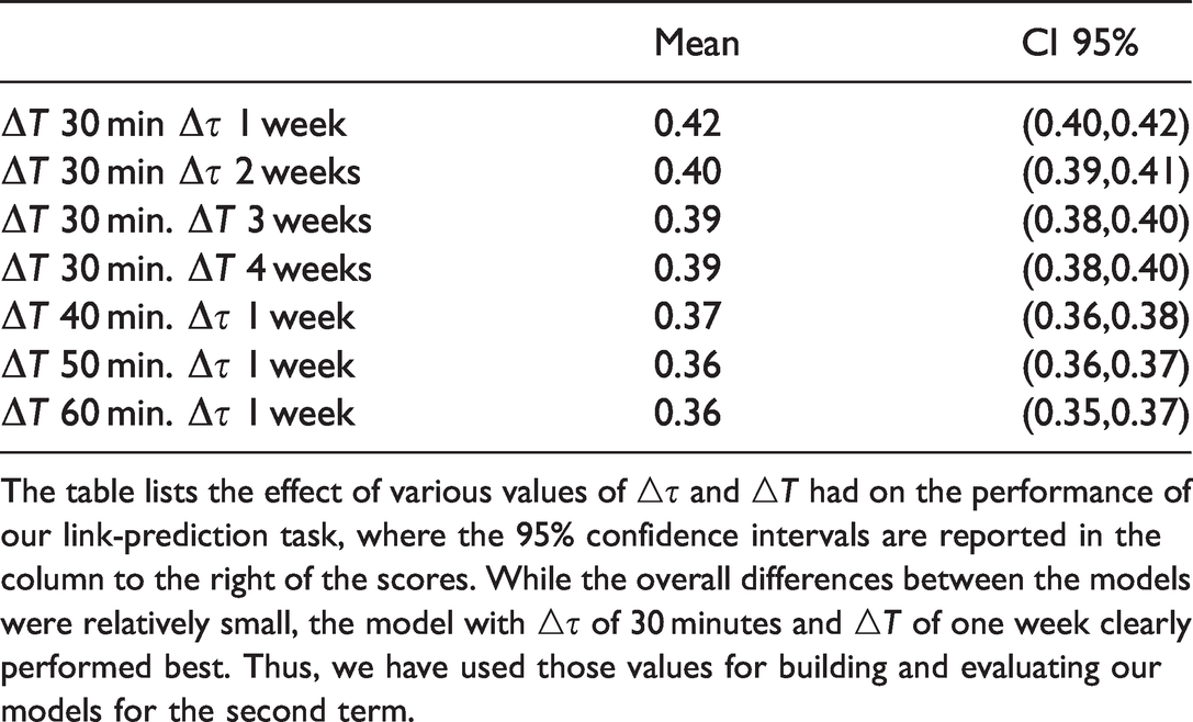
The table lists the effect of various values of $△ τ$ and $△ T$ had on the performance of our link-prediction task, where the 95% confidence intervals are reported in the column to the right of the scores. While the overall differences between the models were relatively small, the model with $△ τ$ of 30 minutes and $△ T$ of one week clearly performed best. Thus, we have used those values for building and evaluating our models for the second term.

Model construction

In order to test the importance of each domain for predicting future encounters, we constructed several different models. Each of the models we built has access to a different set of features. Should the context of an encounter have played a role than our contextual features should have also been relevant for predicting future encounters. Table 3 lists each model and its corresponding features and also indicates, if the feature was derived using $△ T$ or $△ τ$ as a feature preparation interval.

Table 3.

Model features.

Feature	Base	Node	Soc.	Spat.	Temp.	Con.	Net.	Full	Ref.	$△ τ$	$△ T$
Edge	x	x	x	x	x	x	x	x		x
Recency	x	x	x	x	x	x	x	x		x
Time spent together.	x	x	x	x	x	x	x	x		x
Current hour		x			x	x		x			x
Hour-of-the-day vector		x			x	x		x		x
Current weekday		x			x	x		x			x
Day-of-week vector		x			x	x		x		x
Place entropy		x		x		x		x			x
Min (place entropy)		x		x		x		x		x
Relative importance		x		x		x		x			x
MaxRank (relative importance)		x		x		x		x	x	x
Current spatial context		x		x		x		x			x
Time at home tog.		x		x		x		x		x
Time at university tog.		x		x		x		x		x
Time at third places tog.		x		x		x		x		x
Time at other places tog.		x		x		x		x		x
Jaccard similarity		x		x		x		x		x
Avg. amount of people		x	x			x		x	x		x
Triadic periods		0,1,2,3	x			x		x	0,3		x
Preferential attachment							x	x			x
Weighted prop flow							x	x	x		x
Adamic-Adar							x	x			x

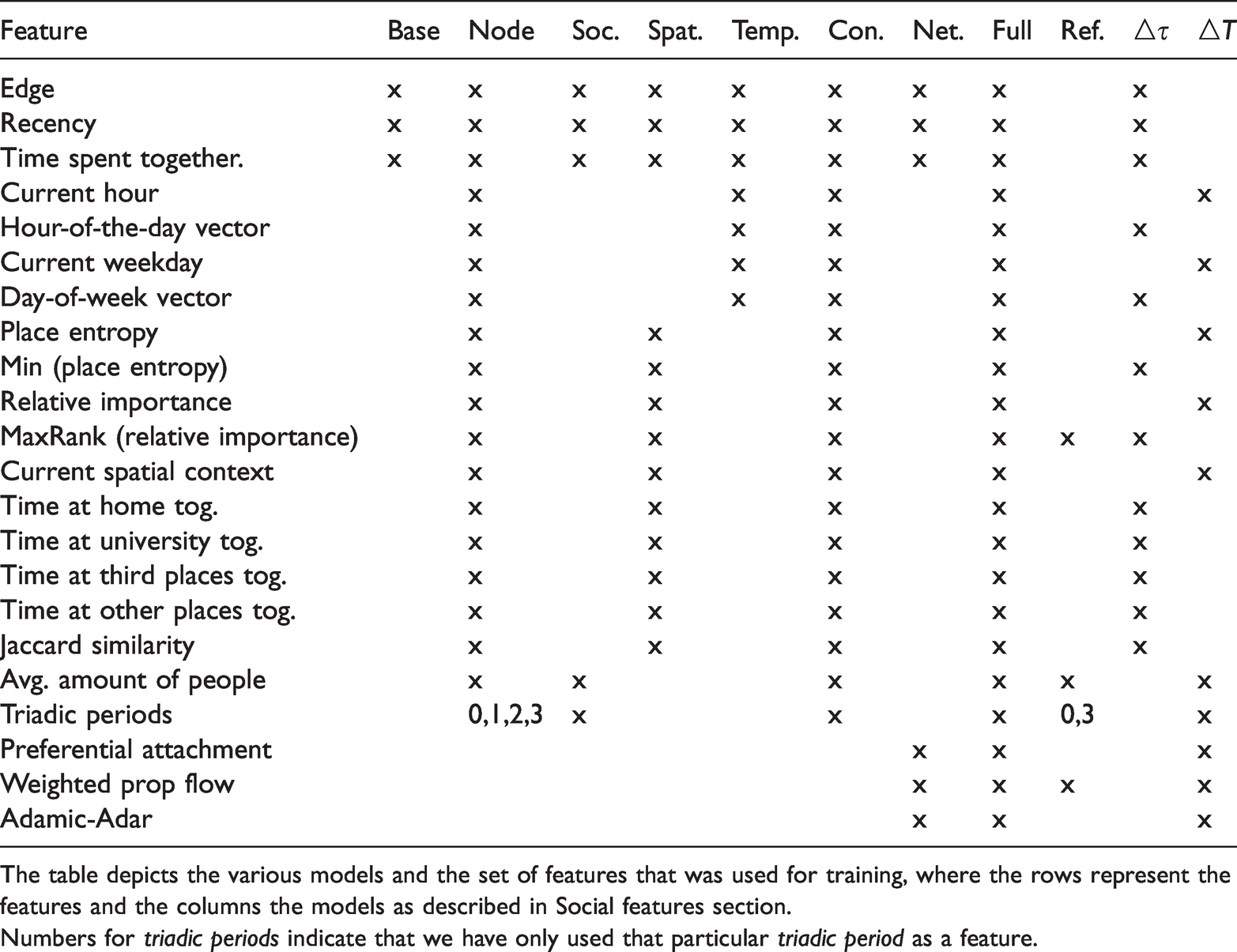
The table depicts the various models and the set of features that was used for training, where the rows represent the features and the columns the models as described in Social features section.

Numbers for triadic periods indicate that we have only used that particular triadic period as a feature.

As a benchmark to test our predictions against we first developed a null model for a time-evolving weighted encounter graph with dissolving ties. Our null model was adapted from Newman and Girvan (2004), where the edges of the graph were randomly rewired under the constraint that the expected degree matches the original degree distribution. In our case, this meant that the expected amount of encounter of each node $u \in G_{t}$ followed the original distribution of meetings, but the encounters between any two nodes $u, v \in G_{t}$ were chosen at random.

Besides the null model, we constructed a base model that only contained the baseline features. We further built a temporal model, a social model, a spatial model and a network topology model by adding to the base models the feature set that pertains to that domain. The context model consisted of the baseline features as well as the temporal, spatial and social features. The full model consisted of all features. We also, after our experiments, constructed a refactored model based on top five features of the full model.

Sometimes one however might not have access to the whole network and might only be in possession of node level data. Hence, one is unable to calculate or reliably estimate the features that utilise the wider network topology we described above. We simulated such a scenario by building node model that only incorporated features that could be obtained from the ego-network of a node. In particular, the features for the node model were: The baseline features, and all the spatial, temporal and social features with the limitation that ‘triad 4’ could not be distinguished from ‘triad 1’ and ‘triad 5’ not from ‘triad 3’.

Findings

To compare the performance of our different models we chose to report the precision, the recall, the precision–recall curve and the area under the precision–recall curve (PR AUC), where precision is plotted on the y-axis and recall on the x-axis (Davis and Goadrich, 2006). Precision and recall are defined as follows (Davis and Goadrich, 2006): In a binary classification task, true positives (TP) are instances correctly labelled as positives, whereas false positives (FP) are incorrectly labelled as positives. Conversely, true negatives (TN) are examples correctly labelled as negatives and false negatives (FN) refer to positive examples erroneously labelled as negatives. Recall is then $\frac{T P}{T P + F N}$ and precision $\frac{T P}{T P + F P}$ .

The area under the PR curve can then be directly used to compare the performance of different models (i.e. the bigger the area the better the model) and is suited to evaluate the performance of an algorithm if there is a large class imbalance as in our data (Davis and Goadrich, 2006).

Performance of the link-prediction algorithm

First, all models performed significantly better than the null model; however, only the network model had a higher PR AUC score than the base model (Figure 1 as well as Table 4). Unsurprisingly, nodes are not randomly interacting with other nodes but exhibit learnable patterns (at least to a certain degree).

Figure 1.

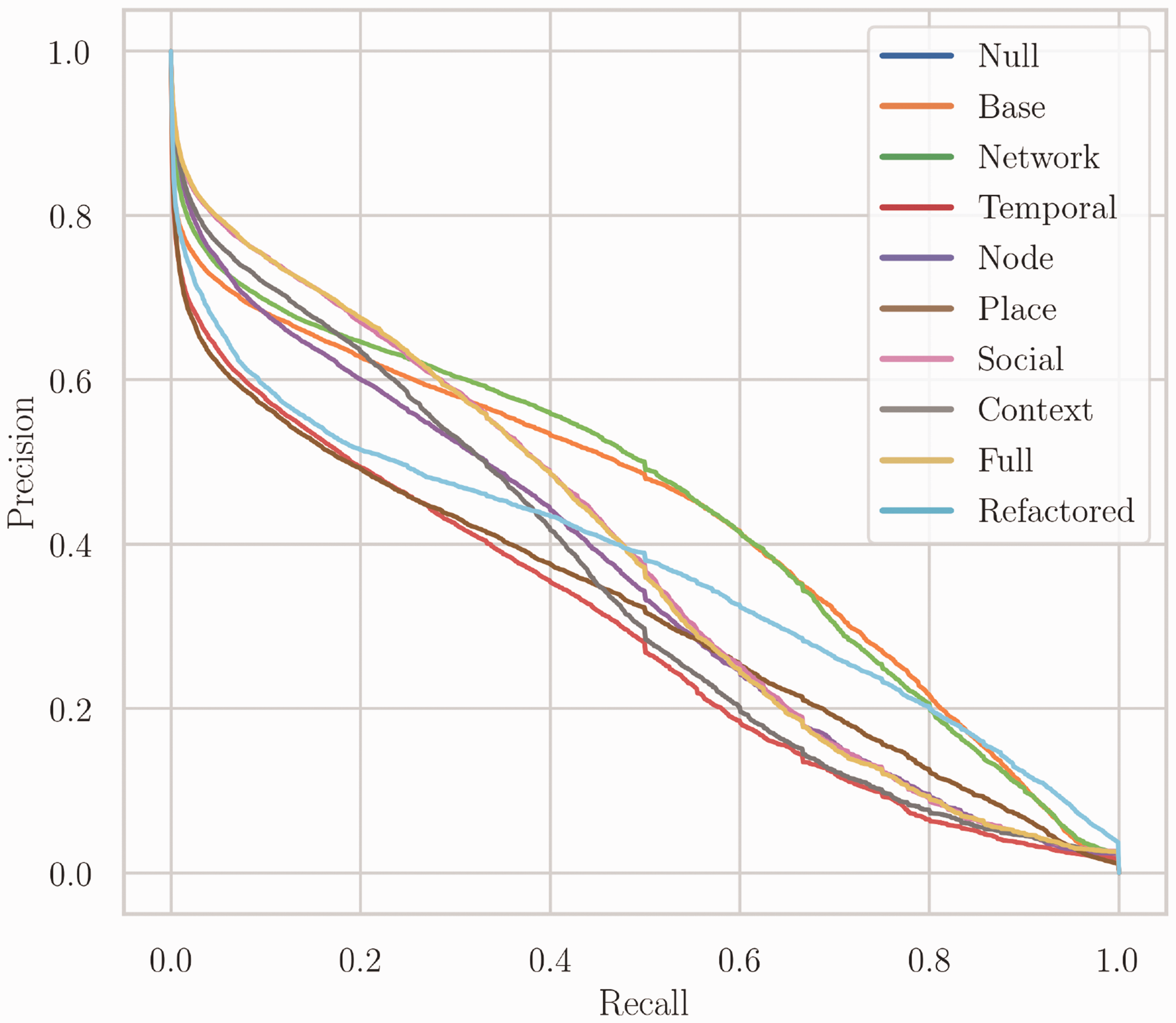
Precision recall curves. The figure depicts the precision-recall curves of the different models. As we fitted a separate tree R for each student, these curves were built by averaging the individual PR curves of each R. The network model performed best, while the base model was only slightly worse overall; in particular those two models managed to keep a relatively high precision score for higher recall values. The social and full model had relatively high precision scores as well.

Table 4.

Model scores.

	${\bar{x}}_{Precision}$	CI 95%	${\bar{x}}_{Recall}$	CI 95%	${\bar{x}}_{P R}$	CI 95%
Null	0.00	(0.00,0.00)	0.00	(0.00,0.00)	0.00	(0.00,0.00)
Base	0.13	(0.12,0.13)	0.69	(0.68,0.70)	0.41	(0.40,0.42)
Network	0.20	(0.20,0.21)	0.71	(0.70,0.72)	0.38	(0.37,0.39)
Time	0.08	(0.08,0.08)	0.74	(0.73,0.74)	0.42	(0.42,0.43)
Node	0.14	(0.14,0.15)	0.71	(0.70,0.72)	0.36	(0.34,0.36)
Place	0.07	(0.07,0.08)	0.65	(0.64,0.66)	0.30	(0.28,0.30)
Social	0.03	(0.04,0.04)	0.77	(0.76,0.77)	0.32	(0.32,0.34)
Context	0.20	(0.20,0.21)	0.71	(0.70,0.72)	0.38	(0.37,0.39)
Full	0.13	(0.12,0.14)	0.60	(0.58,0.60)	0.27	(0.27,0.29)
Refactored	0.13	(0.17,0.19)	0.69	(0.68,0.70)	0.34	(0.33,0.35)

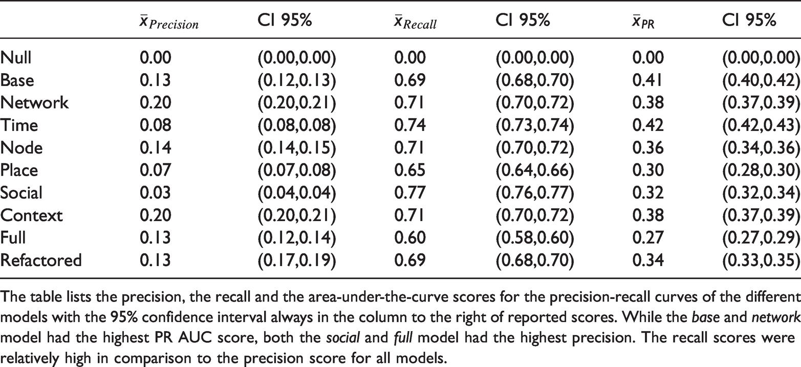
The table lists the precision, the recall and the area-under-the-curve scores for the precision-recall curves of the different models with the 95% confidence interval always in the column to the right of reported scores. While the base and network model had the highest PR AUC score, both the social and full model had the highest precision. The recall scores were relatively high in comparison to the precision score for all models.

Table 5.

The importance of the different features for the full model.

	Mean	CI 95%
Preferential attachment	0.01	(0.01,0.01)
Day of the week	0.01	(0.01,0.01)
Edge	0.04	(0.04,0.04)
Home	0.02	(0.01,0.02)
Current hour	0.02	(0.02,0.02)
Jaccard similarity	0.01	(0.01,0.01)
Max (rel. importance)	0.05	(0.05,0.05)
Met at hour of the day 10	0.01	(0.01,0.01)
Met at hour of the day 14	0.01	(0.01,0.01)
Recency	0.03	(0.03,0.03)
Min (place entropy)	0.04	(0.04,0.04)
Avg. amount of people	0.11	(0.11,0.12)
Place entropy	0.03	(0.03,0.03)
Weighted prop flow	0.11	(0.11,0.11)
Rel. importance	0.04	(0.04,0.04)
Time spent together	0.05	(0.05,0.05)
Time(university)	0.02	(0.02,0.02)
Triadic closure 0	0.10	(0.10,0.10)
Triadic closure 2	0.02	(0.02,0.02)
Triadic closure 3	0.05	(0.05,0.05)
Triadic closure 4	0.02	(0.02,0.02)
Triadic closure 5	0.03	(0.03,0.03)
University	0.02	(0.02,0.02)

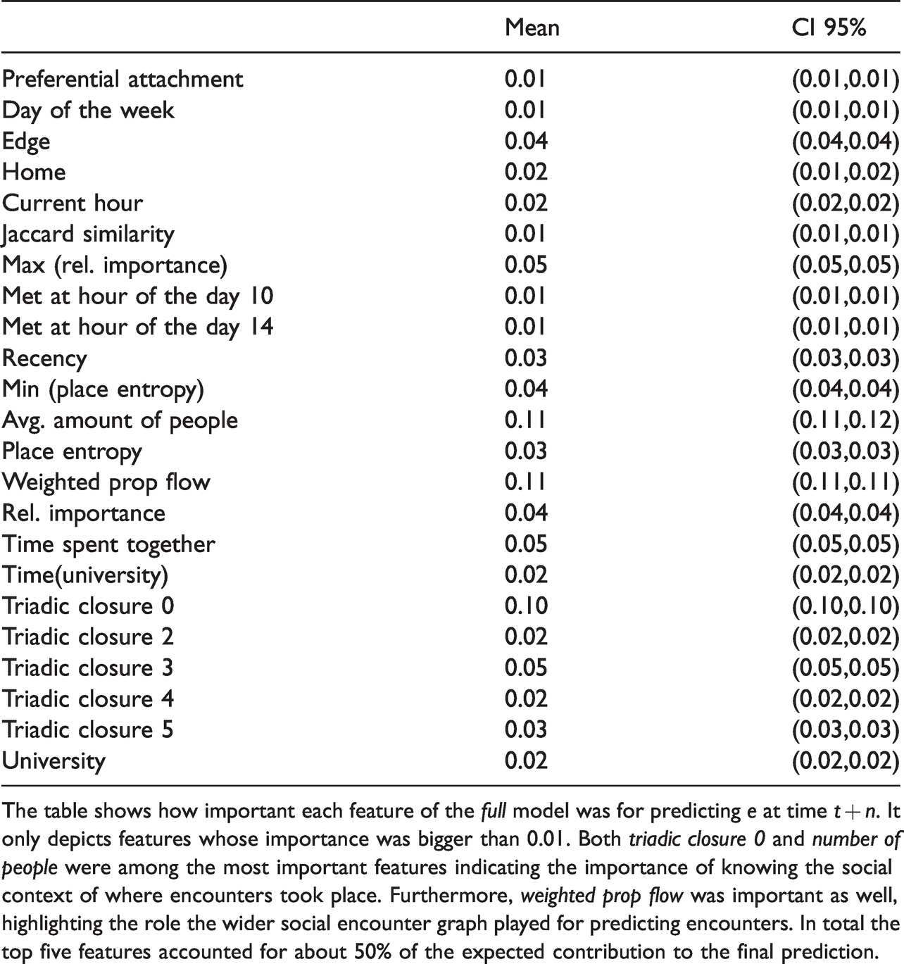
The table shows how important each feature of the full model was for predicting e at time t + n. It only depicts features whose importance was bigger than 0.01. Both triadic closure 0 and number of people were among the most important features indicating the importance of knowing the social context of where encounters took place. Furthermore, weighted prop flow was important as well, highlighting the role the wider social encounter graph played for predicting encounters. In total the top five features accounted for about 50% of the expected contribution to the final prediction.

Second, the models that had the highest PR AUC score were the network and the base model, even though they have access to a lot fewer features than other models. Thus, initially it looked like only a subset of features seemed to be important for the prediction task and some features appeared to even be detrimental for predicting future encounters. The network topology of the social encounter graph G appeared to be very discriminative on its own.

Third, the social and full model had a significantly higher PR AUC score than all models except the base and network model. In particular, with respect to precision both the social and the full model performed much better than any other model, which became apparent not only in the model scores (Table 4) but also in the PRC curves (Figure 1). This indicated that while social features might not have been overall as important as the network topological features, they were still relatively important for correctly predicting whether an encounter occurred.

However, all models had a low precision score compared to the recall scores. This indicated that all models suffered from a relatively large amount of false positives. Given the relatively sparse nature of the social encounter graph G, this finding was not unexpected as there were many more opportunities for false positives than for false positives.

Feature importance

We also investigated the relative importance of the features for predicting future encounters for the full model. Interestingly the top five features – average amount of people, weighted prop flow, triadic closure 0, triadic closure 3 and max(relative importance) accounted for roughly 50% of the expected contribution to the final prediction.

The relative importance of the features was consistent with the low scores for the models that did not include network topological features. Interestingly the social features triadic closure 0 and triadic closure 3 were also important highlighting the process of triadic closure in our dataset and partly explained the comparatively good performance of the social and full model. Triadic closure was consistently shown to be a driving feature of tie formation in networks (Bianconi et al., 2014). This makes sense as when triadic closure occurred, students were already spatially close to each other and thus more likely to encounter each other.

Predicting different types of links

We were also interested in whether the type of relationship (i.e. whether the students were just colleagues, or also socialised outside of university) between nodes affected the predictability of encounters. In order to explore this question, we constructed two new encounter graphs. Recall that G_t was based on all spatial encounters between students regardless of where and when these encounters took place (hereafter $G_{t}^{all}$ ). We constructed $G_{t}^{social}$ based on all the encounters that took place between nodes $u, v \in G_{t}^{social}$ before 9 a.m. or after 6 p.m. local time on weekdays, on the weekend, or in a spatial context other than university. In other words, we were trying to capture the non-university/work related encounters only that happened either after the normal ‘working’ hours, or in a different place than the university. I, furthermore, constructed $G_{t}^{uni}$ that was derived only from encounters between nodes $u, v \in G_{t}^{uni}$ that happened between 9 a.m. and 6 p.m. on weekdays and whose spatial context was university.

Our experiment showed that our model had the highest PC AUC score of 0.49 (0.48–0.49 95% CI) for $G_{t}^{uni}$ followed by a score of 0.38 (0.37–0.39 95% CI) for $G_{t}^{all}$ and a score of 0.34 (0.33–0.35 95% CI) for $G_{t}^{uni}$ . An explanation for the low performance of the model based on $G_{t}^{social}$ could be that ‘social’ encounters are less regular than other encounters; meetings between friends are usually varied in time and place. The performance of the model based on $G_{t}^{uni}$ was significantly better than for any other model. Unsurprisingly students were interacting and meeting regularly; quite likely at the university itself as students from the same year had a similar schedule for lectures.

Discussion

The main finding of our research was that features about whom one meets and the wider network topology of the social encounters significantly improved our predictions, while information about when and where one meets did not seem to play an as important role for our prediction task. Furthermore, and in contrast to previous research that information about where individuals meet did not seem to play a pronounced role for predicting future encounters between individuals in our dataset of students (Scellato et al., 2011b; Yang et al., 2013). It appeared that almost all information was already contained in the network topology of G and the social context rather than in the spatial and temporal setting.

One possible explanation for the relatively low importance of spatial and temporal features could be that as students move through their daily lives, the information of where they are is already embedded in who else is physically close. For example, one is with their partner there is a high chance that one is either at home or at the partner’s home; if one is with their friends from university then there is a high chance that one is meeting them at university. In a sense the social contexts individuals (Sekara et al., 2016) inhabit might intrinsically be linked to spatial places. A competing interpretation for our findings could be that as students are already sharing a lot of places, lectures at the university, for this particular demographic additional opportunity to interact might be less relevant.

Our findings highlight the importance to account for the social embedding of ties for studying mobility behaviour. Specifically, our result indicate the importance of jointly assessing spatial, temporal and social features in order to understand the dynamics of social encounters because human interactions can be spatially, temporally and socially confounded with each other. Such a perspective is usually ignored by mobility studies. Applications that might be informed by our findings range from modelling travel behaviour over understanding the spread of communicable diseases to spatial planning. In essence, applications wherein an understanding of both social as well as mobility behaviour is required for accurately modelling human behaviour can benefit from jointly considering spatial, temporal and social features.

Carrasco et al. (2008) argued that it is important for understanding travel behaviour to study ‘the composition and structure of the personal networks in which these ties are embedded’. Building upon that notion, and while out of scope for this work, one interesting route to explore would thus be to not only map but also conceptualise human behaviour not in the traditional dimensions of time and space as in time-geography (Hägerstrand, 1970) but in a reference frame of time, social and spatial dimensions.

The performance of our link-prediction algorithm was significantly better when considering all ties rather than just social ties but worse than when considering just university ties. We believe that a better understanding the role different types of relationships play for encounters could be a fruitful avenue for future research.

Last, addressing potential other factors such as the weather, the wider social context an interaction takes place in, and might shed light on dynamics that we could not account for in our study. Thus, studying those factors and their relationship with predicting future encounters would also be an interesting topic for future research.It is an open question whether potential other factors such as the weather or can help improve the prediction of social ties.

However, one has to be careful when generalising from our sample of students to the whole population. While we were not aware of any reason our findings should not also hold for broader population groups, the dataset in our study represented after all just one sample of a network. Furthermore, our classification of geographic places was rather broad and did not allow for a detailed analysis of those factors. We believe that a more fine-grained analysis of the role of geographic place is an interesting prospect for future research, especially in conjunction with an expanded analysis of the predictability of different types of ties.

Table 1.

Descriptive statistics of the features.

Feature	Q1	Q2	Q3	Max	Mean	SD
Edge	0.00	0.00	0.00	1.00	0.00	0.02
Recency	0.00	0.00	317,291.0	8,153,620.00	546,661.99	1,239,476.43
Time spent together	0.00	0.00	0.00	454,905.00	178.15	2780.26
Met at hour of the day 0	0.00	0.00	0.00	141.00	0.02	0.74
Met at hour of the day 1	0.00	0.00	0.00	143.00	0.02	0.78
Met at hour of the day 2	0.00	0.00	0.00	139.00	0.02	0.79
Met at hour of the day 3	0.00	0.00	0.00	141.00	0.02	0.82
Met at hour of the day 4	0.00	0.00	0.00	141.00	0.02	0.84
Met at hour of the day 5	0.00	0.00	0.00	143.00	0.02	0.87
Met at hour of the day 6	0.00	0.00	0.00	141.00	0.02	0.87
Met at hour of the day 7	0.00	0.00	0.00	141.00	0.02	0.87
Met at hour of the day 8	0.00	0.00	0.00	137.00	0.02	0.78
Met at hour of the day 9	0.00	0.00	0.00	136.00	0.05	0.92
Met at hour of the day 10	0.00	0.00	0.00	114.00	0.07	1.03
Met at hour of the day 11	0.00	0.00	0.00	111.00	0.09	1.15
Met at hour of the day 12	0.00	0.00	0.00	111.00	0.09	1.13
Met at hour of the day 13	0.00	0.00	0.00	105.00	0.07	0.97
Met at hour of the day 14	0.00	0.00	0.00	102.00	0.08	1.08
Met at hour of the day 15	0.00	0.00	0.00	100.00	0.09	1.11
Met at hour of the day 16	0.00	0.00	0.00	99.00	0.07	1.04
Met at hour of the day 17	0.00	0.00	0.00	96.00	0.06	0.92
Met at hour of the day 18	0.00	0.00	0.00	113.00	0.03	0.72
Met at hour of the day 19	0.00	0.00	0.00	107.00	0.02	0.64
Met at hour of the day 20	0.00	0.00	0.00	107.00	0.02	0.64
Met at hour of the day 21	0.00	0.00	0.00	132.00	0.02	0.67
Met at hour of the day 22	0.00	0.00	0.00	137.00	0.02	0.67
Met at hour of the day 23	0.00	0.00	0.00	138.00	0.02	0.70
Place entropy	0.00	0.14	3.39	9.05	2.10	3.03
Min (place entropy)	0.00	0.00	0.00	9.05	0.38	1.68
Rel. importance	0.00	0.47	0.76	1.00	0.40	0.36
Max (rel. importance)	0.00	0.00	0.00	1.00	0.01	0.05
Home	0.00	1.00	1.00	1.00	0.55	0.50
University	0.00	0.00	0.00	1.00	0.09	0.29
Third place	0.00	0.00	0.00	1.00	0.02	0.15
Other place	0.00	0.00	1.00	1.00	0.34	0.47
Time at home tog.	0.00	0.00	0.00	377,708.00	52.95	2137.18
Time at university tog.	0.00	0.00	0.00	283,323.00	101.12	1291.56
Time at third places tog.	0.00	0.00	0.00	248,728.00	0.17	121.96
Time at other places tog.	0.00	0.00	0.00	345,246.00	6.27	591.79
Jaccard similarity	0.00	0.07	0.14	1.00	0.08	0.09
Avg. amount of people	0.00	0.00	0.00	22.00	0.00	0.14
Triadic period 0	6.00	6.00	6.00	6.00	5.17	1.86
Triadic period 1	0.00	0.00	0.00	5.00	0.00	0.02
Triadic period 2	0.00	0.00	0.00	6.00	0.00	0.06
Triadic period 3	0.00	0.00	0.00	6.00	0.00	0.08
Triadic period 4	0.00	0.00	0.00	119.00	0.01	0.25
Triadic period 5	0.00	0.00	0.00	89.00	0.00	0.20
Preferential attachment	0.00	0.00	0.00	396.00	0.32	3.00
Weighted prop flow	0.00	0.00	0.00	0.38	0.00	0.01
Adamic-Adar	0.00	0.00	0.00	10.10	0.00	0.03

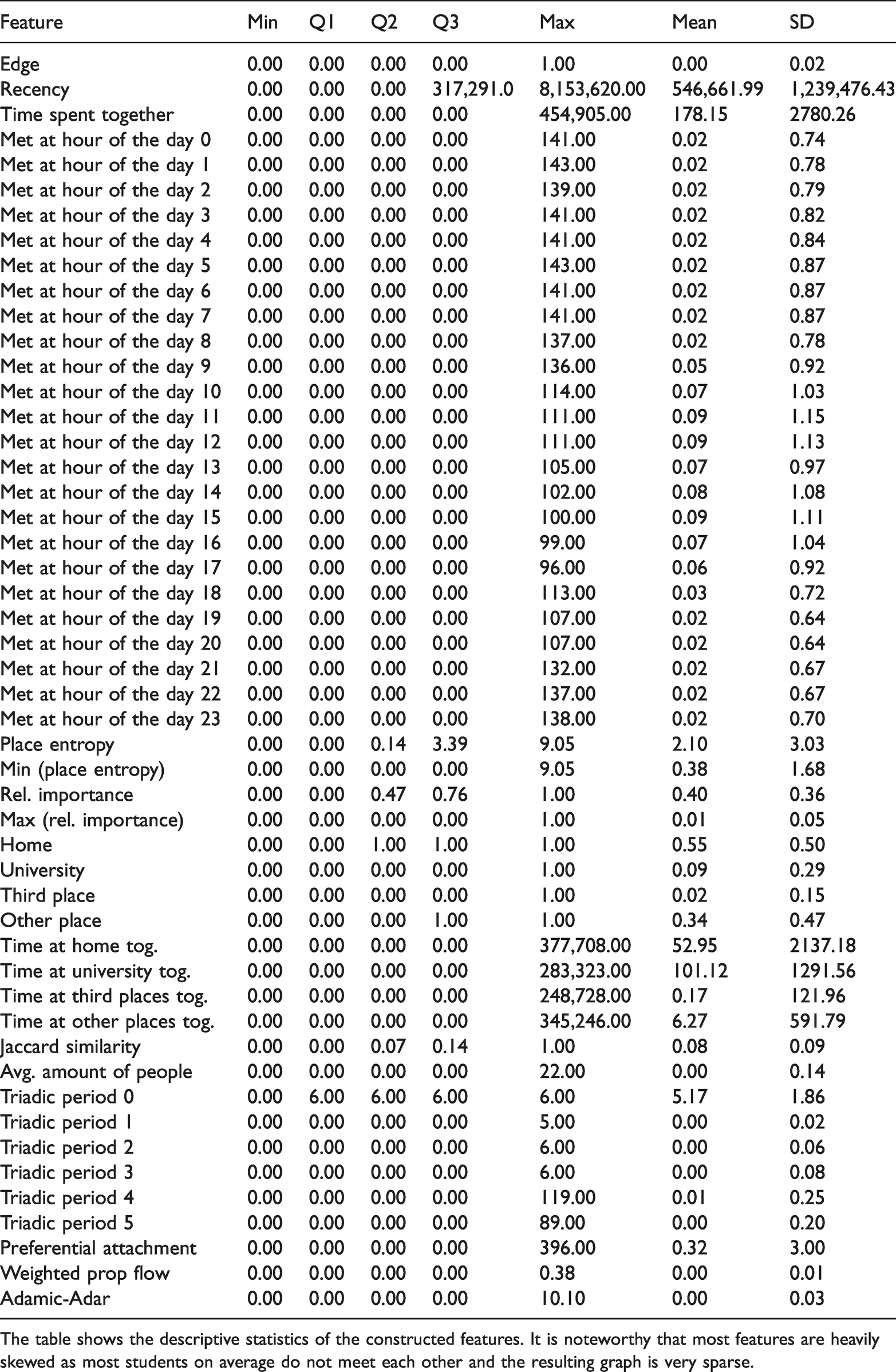
The table shows the descriptive statistics of the constructed features. It is noteworthy that most features are heavily skewed as most students on average do not meet each other and the resulting graph is very sparse.

Footnotes

Declaration of conflicting interests

The author(s) declared no potential conflicts of interest with respect to the research, authorship, and/or publication of this article.

Funding

The authors disclosed receipt of the following financial support for the research, authorship, and/or publication of this article: This research was in part supported by an Economic and Social Research Council PhD scholarship (ES/J50001X/1).

Note

Biographical notes

Christoph Stich: I was a PhD student at the University of Birminhgam studying the interplay of social networks and human mobility. Since graduating I have been working on implementing the state-of-the-art in Poker AI as a commercial product.

Emmanouil Tranos: I am a Reader in Quantitative Human Geography at the University of Bristol and a Fellow at the Alan Turing Institute. My research has been exposing the spatial dimensions of digital technologies and the digital economy from their early stages until today. I have published on issues related to the geography of the internet infrastructure, the economic impacts that such digital infrastructure can generate on cities and regions and the position of cities within spatial, complex networks

Mirco Musolesi: I am Professor of Computer Science at the Department of Computer Science at University College London (UCL). I am a Turing Fellow at the Alan Turing Institute, the UK National Institute for Data Science and Artificial Intelligence. I am the Turing University Lead for UCL. I am also Professor of Computer Science at the Department of Computer Science and Engineering at the University of Bologna.

Sune Lehmann: I’m a Professor of Networks and Complexity Science at DTU Compute, Technical University of Denmark. I’m also a Professor of Social Data Science at the Center for Social Data Science (SODAS), University of Copenhagen. My work focuses on quantitative understanding of social systems based on massive data sets. A physicist by training, my research draws on approaches from the physics of complex systems, machine learning, and statistical analysis.

References

Adams

Faust

Lovasi

(2012) Capturing context: Integrating spatial and social network analyses. Social Networks 34(1): 1–5.

Alessandretti

(2018) Individual mobility in context: From high resolution trajectories to social behaviour. PhD Thesis, University of London, UK. Available at: http://openaccess.city.ac.uk/20077/ (Accessed on 01.04.2019).

Altmann

Tol Si

Sander

, et al. (2010) Permutation importance: A corrected feature importance measure. Bioinformatics Original Bioinformatics 26(10): 1340–1347.

Arentze

Timmermans

(2008) Social networks, social interactions, and activity-travel behavior: A framework for microsimulation. Environment and Planning B: Planning and Design 35(6): 1012–1027.

Backstrom

Sun

Marlow

(2010) Find me if you can: Improving geographical prediction with social and spatial proximity. In: WWW '10: The 19th International World Wide Web Conference Raleigh North Carolina USA April, 2010, pp. 61–70.

Bapierre

Jesdabodi

Groh

(2015) Mobile homophily and social location prediction measures of social cohesion. arXiv 1–17.

Bianconi

Darst

Iacovacci

, et al. (2014) Triadic closure as a basic generating mechanism of communities in complex networks. Physical Review E 90(042806): 1–10.

Boessen

Hipp

Butts

, et al. (2017) The built environment, spatial scale, and social networks: Do land uses matter for personal network structure? Environment and Planning B: Urban Analytics and City Science 45(3): 1–17.

Breiman

(2001) Random forests. Machine Learning 45(1): 5–32. http://link.springer.com/article/10.1023/A:1010933404324

10.

Brown

Noulas

Mascolo

, et al. (2013) A place-focused model for social networks in cities. In: Proceedings of ICSC’13, 8–14 Sept. 2013, Conference Location: Alexandria, VA, USA, pp. 75–80. http://ieeexplore.ieee.org/lpdocs/epic03/wrapper.htm?arnumber=6693315

11.

Butts

Acton

Hipp

, et al. (2012) Geographical variability and network structure. Social Networks 34(1): 82–100.

12.

Carrasco

Miller

Wellman

(2008) How far and with whom do people socialize?: Empirical evidence about distance between social network members. Transportation Research Record: Journal of the Transportation Research Board 2076: 114–122.

13.

Cho

Myers

Leskovec

(2011) Friendship and mobility: User movement in location-based social networks. In: KDD ’11 proceedings of the 17th ACM SIGKDD international conference on knowledge discovery and data mining, San Diego, US, August 2011, pp. 1082–1090. http://dl.acm.org/citation.cfm?id=2020579

14.

Crandall

Backstrom

Cosley

, et al. (2010) Inferring social ties from geographic coincidences. Proceedings of the National Academy of Sciences of the United States of America 107(52): 22436–22441.

15.

Dankowski

Ziegler

(2016) Calibrating random forests for probability estimation. Statistics in Medicine 35(22): 3949–3960.

16.

Davis

Goadrich

(2006) The relationship between precision-recall and ROC curves. In: ICML ’06 proceedings of the 23rd international conference on machine learning, Pittsburgh, Pennsylvania, June 2006, pp. 233–240.

17.

De Domenico

Lima

Musolesi

(2013) Interdependence and predictability of human mobility and social interactions. Pervasive and Mobile Computing 9(6): 798–807.

18.

Doreian

Conti

(2012) Social context, spatial structure and social network structure. Social Networks 34(1): 32–46.

19.

Eagle

Pentland

(2009) Eigenbehaviors: identifying structure in routine. Behavioral Ecology and Sociobiology 63(7): 1057–1066.

20.

Ester

Kriegel

Sander

, et al. (1996) Density-based clustering methods. In: Proceedings of KDD’96, August 2006, Portland, Oregon, Vol. 2, pp. 226–231.

21.

Glover

Parry

(2009) A third place in the everyday lives of people living with cancer: Functions of Gilda’s Club of Greater Toronto. Health & Place 15(1): 97–106.

22.

Hägerstrand

(1970) What about people in regional science? Papers in Regional Science 24(1): 7–21.

23.

(2002) A data complexity analysis of comparative advantages of decision forest constructors. Pattern Analysis & Applications 5(2): 102–112.

24.

Hyndman

Athanasopoulos

(2013) Forecasting: Principles and Practice. Melbourne: OTexts.

25.

Isella

Stehle

Barrat

, et al. (2011) What’s in a crowd? Analysis of face-to-face behavioral networks. Journal of Theoretical Biology 271(1): 166–180.

26.

Kowald

van den Berg

Frei

, et al. (2013) Distance patterns of personal networks in four countries a comparative study. Journal of Transport Geography 31: 236–248.

27.

Lambiotte

Blondel

de Kerchove

, et al. (2008) Geographical dispersal of mobile communication networks. Physica A: Statistical Mechanics and Its Applications 387(21): 5317–5325.

28.

Larsen

Urry

Axhausen

(2006) Mobiliites, Networks, Geographies. Hampshire / Burlington, VT: Ashgate. http://scholar.google.com/scholar?hl=en&btnG=Search&q=intitle:No+Title#0http://scholar.google.com/scholar?hl=en%7B&%7DbtnG=Search%7B&%7Dq=intitle:No+Title%7B#%7D0

29.

Mair

(2009) Club life: Third place and shared leisure in rural Canada. Leisure Sciences 31(5): 450–465.

30.

Newman

MEJ

Girvan

(2004) Finding and evaluating community structure in networks. Physical Review E 69(026113): 1–16.

31.

Noulas

Shaw

Lambiotte

, et al. (2015) Topological properties and temporal dynamics of place networks in urban environments. In: WWW '15: 24th International World Wide Web Conference Florence Italy May, 2015, pp. 431–44.

32.

Oldenburg

Brissett

(1982) The third place. Qualitative Sociology 5(4): 265–284.

33.

Pedregosa

Varoquaux

(2011) Scikit-learn: Machine learning in python. The Journal of Machine Learning Research 12: 2825–2830.

34.

Peng

(2015) Link prediction in social networks: The state-of-the-art. SCIENCE China Information Sciences 58(011101): 1–38.

35.

Ranjan

Zang

Zhang

, et al. (2012) Are call detail records biased for sampling human mobility? ACM SIGMOBILE Mobile Computing and Communications Review 16(3): 33.

36.

Reis

Wheeler

(1991) Studying social interaction. Advances in Experimental Social Psychology 24: 269–318.

37.

Rosenbaum

Ward

Walker

, et al. (2007) A cup of coffee with a dash of love. Journal of Service Research 10(1): 43–59.

38.

Scellato

Noulas

Lambiotte

, et al. (2011a) Socio-spatial properties of online location-based social networks. In: Proceedings of the 5th international AAAI conference on weblogs and social media – ICWSM ’11, July 17–21, 2011 in Barcelona, Catalonia, Spain, pp. 329–336.

39.

Scellato

Noulas

Mascolo

(2011b) Exploiting place features in link prediction on location-based social networks categories and subject descriptors. In: Proceedings of KDD’11, pp. 1046–1054.

40.

Sekara

Lehmann

(2014) The strength of friendship ties in proximity sensor data. PLoS ONE 9(7): e100915.

41.

Sekara

Stopczynski

Lehmann

(2016) The fundamental structures of dynamic social networks. Proceedings of the National Academy of Sciences 113(36): 9977–9982.

42.

Stehle

Voirin

Barrat

, et al. (2011) High-resolution measurements of face-to-face contact patterns in a primary school. PLoS ONE 6(8): e23176.

43.

Stopczynski

Sekara

Sapiezynski

, et al. (2014) Measuring large-scale social networks with high resolution. PloS ONE 9(4): e95978.

44.

Toole

Herrera-Yaqu

Schneider

, et al. (2015) Coupling human mobility and social ties. Journal of the Royal Society Interface 12: 20141128–20141129.

45.

Wang

Pedreschi

Song

, et al. (2011) Human mobility, social ties, and link prediction categories and subject descriptors. Proceedings of KDD’ 11, San Diego California USA August, 2011, pp. 1100–1108.

46.

Yang

Chawla

Basu

, et al. (2013) Link prediction in human mobility networks. In: Proceedings of ASONAM 2013, Niagara Ontario Canada August, 2013, pp. 380–387.

47.

Zhao

Stehlé

Bianconi

, et al. (2011) Social network dynamics of face-to-face interactions. Physical Review E 83(56109): 1–18.