Sage Journals: Discover world-class research

Abstract

The research presented in this paper addresses a current gap in the availability of building geometry data and provides estimates of individual building characteristics at city scale. Such data are crucial for a wide range of subjects such as modelling building energy consumption as well as regional housing market studies. However, such data are currently not available in the UK. In this work, a new approach was developed to automatically estimate the geometric characteristics of buildings, including height and floor count. A wide range of datasets have been brought together including high-resolution light detection and ranging data to accurately estimate building elevation and to obtain the external dimension of buildings. In the UK, most of the datasets required for this model are available for urban areas, allowing the model to be widely applied both in cities and beyond. The paper presents the results of building height and floor count determined from this model and compares these with the actual data obtained from a survey of 108 representative buildings in the city of Southampton. The results show good accuracy of the model with 97% of the estimates having an error under ±1 floor and an absolute mean error of 0.3 floors. These results provide confidence in utilising this model for future building studies at a city scale.

Keywords

Built environment cities geographic information system model validation remote sensing

Introduction

Characteristics of building internal space such as total floor area and the floor count (number of floors) are important factors for a wide range of studies such as house price analysis (Orford, 2010) and building energy simulations (Balaras et al., 2005; Hong et al., 2006; Jaggs and Palmer, 2000). Detailed information on urban building pattern is also essential for city-scale analysis including urban planning and socio-economic analysis (Wu et al., 2017a). However in the UK, there is a paucity of such data (González-Aguilera et al., 2013; Orford, 2010). Existing datasets cannot be directly used to obtain internal attributes of individual buildings at city, or larger, scales. As a result, research into city-scale building stocks often adopt various methods to estimate building dimensional characteristics, but the accuracy of these methods remains uncertain. For example, building height information in the model of Iowerth et al. (2013) was extracted from the UK Building Classification dataset provided by the Geoinformation Group (2014). This dataset, however, has low spatial resolution as it separates buildings into district-level areas and assigns unified height values to all buildings in the area. As a result, this dataset is not able to provide elevation data for individual buildings. Using a different approach, a number of studies such as Gupta and Gregg (2014) and Hong et al. (2006) chose to conduct on-site surveys to obtain actual building data, but such an approach could only be conducted on a limited number of sample buildings and is difficult to apply widely and at scale. Reinhart and Cerezo Davila (2016) also reviewed recent works that are based on a different approach by separating buildings in a city into a number of archetypes, but such approach would still require considerable manual effort and statistical building data and would not be able to reflect the characteristics of each individual building within a city. To address this challenge, Iannelli and Dell’Acqua (2017) developed a deep learning methodology using street view images at scale, and their model was able to estimate the number of floors for individual buildings based on visual interpretation.

In 2014, the Ordnance Survey (OS) as part of their MasterMap® dataset published an alpha version of building height dataset. This dataset has not been widely adopted in city-scale building studies, and its results require further assessments to validate the methodology utilised. The OS dataset uses digital terrain model (DTM) to estimate the altitude of bare earth surfaces, and the DTM was derived from digital surface model (DSM) by using interpolation methodologies (Galvanin and Dal Poz, 2011). Such an approach, however, as demonstrated by Chen et al. (2012) is likely to have low accuracy and the results may contain significant errors due to the influence of undetected buildings or other objects such as trees. Meng et al. (2010) reviewed current works on ground surface detection and summarised the most typical error sources from DTM interpolation, which include the influence of shrubs, short walls, bridges, and the fact that most interpolation works lack reliable accuracy assessment. It is further demonstrated by Truong-Hong and Laefer (2015) that building detection methodologies, even with the utilisation of high-density datasets, could have limited accuracy in identifying certain types of buildings, such as terraced houses with an accuracy of 65%. In addition, the elevation of building roofs in the OS dataset was estimated by combining DSM data with vector data of the outlines of building footprint. This approach, however, overlooks the possibility that the two datasets may not be fully aligned due to errors during the data collection process or due to poor dataset resolution. Furthermore, this approach does not also take into account the influence of objects, such as tree branches, which may extend over building roofs and cause errors. In this work, light detection and ranging (LiDAR) data analysis, coupled with validation surveys of buildings, was conducted to compare the results obtained from the model with that of the OS dataset.

In recent years, a number of building detection methodologies were developed utilising LiDAR data, which uses remote sensing technologies to automatically estimate elevation of objects on the earth surface (Li and Guan, 2011; Sampath and Shan 2010; Siddiqui et al., 2013; Wu et al., 2017a). Huang et al. (2017) separate the aim of such works into two main categories, building characteristics extraction (Chen et al., 2005; Rottensteiner, 2003; Rottensteiner and Briese, 2002) and building classification (Abellán and Moral, 2003; Tobergte and Curtis, 2013; Yan et al., 2016). However, only a limited number of studies were carried out to estimate the floor count in specific buildings. Some of the relevant and existing studies were mainly focused on building roof detection or segmentations, and the reconstruction of buildings in a virtual environment (Amini et al., 2014; Arefi and Reinartz, 2013). For example, Zheng et al. (2017) developed a hybrid approach using LiDAR, building footprint, and orthophotography data to accurately model buildings’ shape and structure. Yu et al. (2010) used DSM and DTM that were derived from LiDAR to generate a normalised DSM layer, which is then used to detect the shape of vegetation and buildings. With the utilisation of multiple thresholds, their model is capable of dealing with buildings that have significant height variations such as high-rise building complexes, which can be seen in numerous urban areas. Their models, however, have not included the conversion from building height to the building floor count (number of floors), which is more closely correlated with the size of living spaces within a building and therefore is an important factor required for various building-level simulations such as for space heating demand or thermal comfort.

González-Aguilera et al. (2013) developed a model using predominantly LiDAR data, and the model is capable of segmenting building roofs into a number of planes. The model uses a roof extraction method (Galvanin and Dal Poz, 2011; Sampath, 2010) to generate outlines of building footprints from DSM. This approach, however, was demonstrated by Orford (2010) to be less accurate than traditional building survey results, such as the MasterMap® data provided by OS for England and Wales. In addition, estimates of building height from the model are not accurate and require users to carry out an additional step for a final review in cases dealing with complex structures. It is also pointed out in Wu et al. (2017b) that models using LiDAR face limitations when dealing with buildings with transparent roofs. Such buildings, however, are very rare to be seen in urban areas in the UK due to climate condition, and therefore are not specifically discussed in this paper.

Orford (2010) developed a model for the application in the UK, which extracts outlines of building footprints from OS MasterMap® and divides them into a series of ‘rectilinear polygons’. The height of each subdivided polygon is then estimated separately. This allowed the model to take into account buildings that consist of multiple structures, e.g. extensions that have different height within a building main body. However, the model described in Orford (2010) uses the median value of LiDAR points associated with a building’s roof to represent the roof elevation. But this value, unlike the elevation of roof base (e.g. eaves), does not directly correlate with the volume of living spaces within the building as the slope of each roof varies.

In this work, a model was developed to automatically estimate the geometry of individual buildings. The model detects not only the elevation of a building roof but also the ground surfaces on which the main construction part of the building stands, namely the building base. It does not rely on DTM data that are obtained by interpolating DEM data, but directly detects ground surfaces that are close to the base of a building. A tier-based methodology is further developed to convert the obtained building heights into estimates of the floor count. The results of the modelling were validated by comparing with actual building data obtained from surveys of randomly selected sample buildings in Southampton, UK.

Methodology

Figure 1 shows modelling processes used within the model to estimate height and floor count of buildings. The model uses predominantly two GIS-based datasets: a shapefile of building outlines provided as part of OS MasterMap® (Ordnance Survey, 2014) and LiDAR data provided by the Environment Agency (2013) as input data, both of which are widely available in UK urban areas. The MasterMap® provides a detailed vector layer containing the outline of buildings in the format of polygons, which are results of continuous manual survey works by OS. The LiDAR datasets were generated from a series of surveys carried out by the Environment Agency in 2015, and the point cloud has a resolution of 1 m (Environment Agency, 2013). In this work, the two datasets are spatially merged to identify LiDAR points that fall within the outline of a building. These points represent the elevation of surface areas that are either on top of a building roof or in close proximity to a building.

Figure 1.

Flowchart of processes developed in the model where building outline is obtained from OS MasterMap® (Ordnance Survey, 2014), LiDAR obtained from the Environment Agency (2013). LiDAR: light detection and ranging; OS: Ordnance Survey.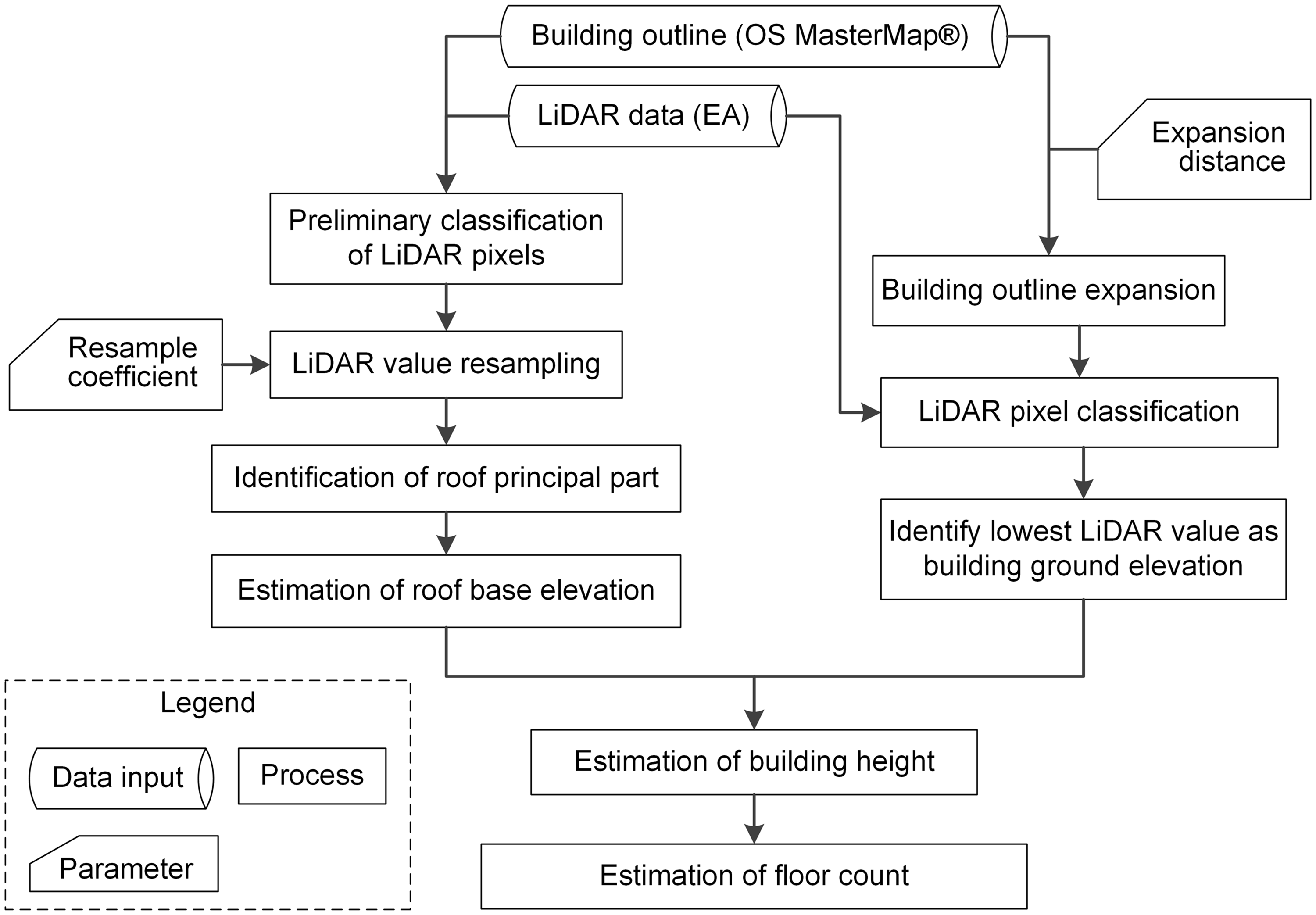

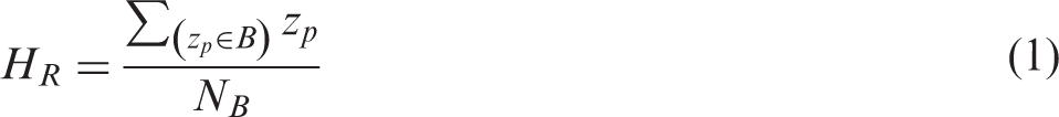
To identify the base height of a building’s roof, the model resamples the values of LiDAR points that are enclosed within a building outline into a number of bands so that small variations caused by components that have similar elevations can be taken into account. A statistical analysis is then carried out to identify the most frequently repeated elevation band for each building, and LiDAR points included in this band are used to represent the principal part of the building roof which is most likely to be, or close to, the roof base. This approach is designed to take into account the diversity of roof geometries and to avoid the influence of various forms of protrusions caused by objects that are likely to be installed on top of a roof surface such as chimney and machinery, as well as trees. The elevation of a building roof is estimated by calculating the average elevation of all LiDAR points in the principal roof areas, and this process is described by equation (1)

\begin{matrix} H_{R} = \frac{\sum_{(z_{p} \in B)} z_{p}}{N_{B}} \end{matrix}

(1)

where H_R is the roof base elevation, z_p denotes the elevation of individual LiDAR points, B is the principal roof elevation band, and N_B is the number of LiDAR points included in this band.

To estimate the elevation of the base of buildings (ground level), a new approach has been developed to identify ground surfaces that are in close proximity to individual buildings, rather than to generate a complete DTM for the bare earth surfaces in a city. This reduces significantly the computation time needed to study a region and avoids errors that could be caused due to interpolation of geographic terrain. In this approach, the footprint outline of a building (base) is expanded by a small distance of 1 m (expansion coefficient in Figure 1), and the LiDAR data enclosed within the expanded area are extracted for further analysis. The lowest point within this area represents the ground surface, and its elevation is used as the elevation of the base of individual buildings.

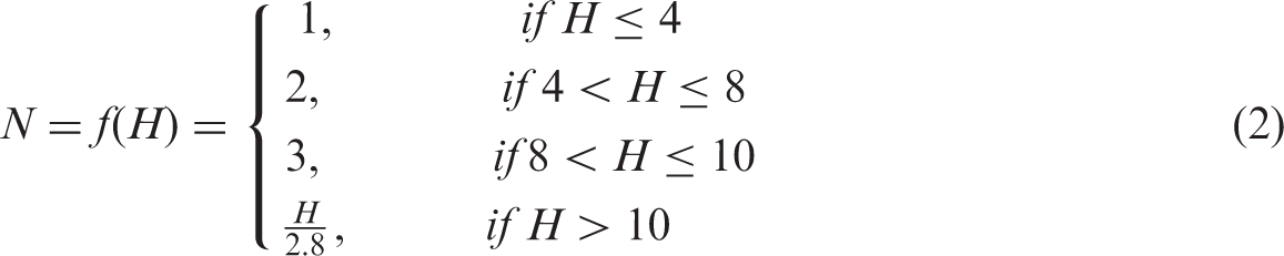
The net height of a building, which is equal to the difference between roof elevation and ground surface elevation, is then utilised to estimate the floor count of each building. This conversion is illustrated by equation (2)

\begin{matrix} N = f (H) = {\begin{matrix} 1, & ifH \leq 4 \\ 2, & if 4 < H \leq 8 \\ 3, & if 8 < H \leq 10 \\ \frac{H}{2.8}, & ifH > 10 \end{matrix} \end{matrix}

(2)

where N denotes the estimate of floor count and H denotes the estimated building height. In other words, for buildings under 10 m, the model uses a tier-based algorithm (equation (2)) with thresholds set at 4 m (floor count = 1), 8 m (floor count = 2), and 10 m (floor count = 3), respectively. This is to take into account the variation of unit height of a single floor, which can be found among buildings constructed at different periods, and errors in the estimate of H (Department for Communities and Local Government, 2017). For buildings that are over 10 m, the model uses a linear equation (last section of equation (2), i.e. N = H/2.8) to convert building height into floor count. The value of 2.8 m was chosen based on floor height data extracted from bulk Energy Performance Certificate datasets by the UK government (Department for Communities and Local Government, 2017), in which the average height of each floor in domestic buildings was found to be in the range 2.6–2.9 m, varying with geographic location. Results from this conversion will be presented as fractional values, giving flexibility to the model results in predicting buildings that have inconsistent floor structure, as discussed further in ‘Buildings with multiple roof sections’ section.

Results and analysis

The floor count in each building is estimated by the model utilising the results derived from building height estimates. As the floor count correlates strongly with the size of living spaces within a building, it is an important factor for the simulation of the thermal energy in buildings. However, although the floor count of buildings can be recognised easily by visual inspection, undertaking such a task for all buildings in a city will be cumbersome and labour intensive. As this type of data for buildings are not available for all individual buildings within a city, the model presented in this paper is intended to address this gap of knowledge. In order to test the accuracy of the model of estimating the floor count of a building, visual external observations (surveys) were carried out on a sample of buildings in Southampton and the results were compared with model estimates. Prior to this test, the performance of the model in identifying building roof base has been tested, and the results and discussions are presented in online supplementary material.

Sample selection and surveys

In order to attain a representative sample size of buildings for the City of Southampton, a method proposed by Liang and Shen (2012), which is based on well-established statistical methods for calculating required sample sizes (Kreyszig et al., 2011) but simplified to suit building studies with large population and sample size. The method introduced in Liang and Shen (2012) is shown in equation (3)

n = \frac{t^{2} s^{2}}{Δ_{\bar{x}}^{2}}

(3)

where n is the required sample size,

Δ_{\bar{x}}

is the confidence interval, t is the degree of probability, and s is the standard deviation of the sample.

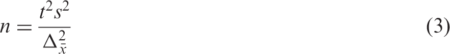
This method is deemed to achieve a 95% of confidence in representation with a 10% of error margin. The validation process is further improved by separating residential buildings in Southampton into five categories namely:

Detached houses (stand-alone buildings that do not share a wall with other buildings).

Semi-detached houses (with one wall shared with the next building).

Terraced houses (buildings sandwiched between the two adjacent properties – both sidewalls shared).

Low-rise multi-occupancy buildings or flats (apartments) with floor count ≤ 3.

Medium- and high-rise multi-occupancy buildings or towers of flats with the floor count > 3.

The above classification encompassed 30,912 buildings in the city. The required sample sizes stipulated by Liang and Shen (2012) methodology for each classification and the results of the analysis of the model are shown in Table 1. The estimated results of the floor count for terraced houses and semi-detached houses have standard deviation of 0.28 and 0.24, respectively, indicating that these buildings have similar values in terms of floor count, and the sample size of buildings required is 7 and 6, respectively. These sample sizes were derived from sampling the entire terrace instead of individual properties. High-rise buildings, however, have much higher standard deviation in the estimated floor count, and therefore the samples of buildings needed are 62 buildings. Conversely, for low-rise multi-occupancy buildings of flats and detached houses the required sample sizes are 17 and 26, respectively.

Table 1.

Building type and the sample size required to validate the estimated floor count of a building by the model.

	Mean (95% CI)	St dev (95% CI)	Total no. of buildings	Sample size
Detached house	1.76 (1.61,1.93)	0.46 (0.33,0.56)	11,391	26
Semi-detached house	1.97 (2.00,2.00)	0.24 (0,0)	11,180	6
Terraced house	2.03 (1.60,2.12)	0.28 (0.07,0.88)	3899	7
Low-rise flat	2.16 (2.13,2.70)	0.46 (0.47,0.81)	3704	17
High-rise flat	4.64 (3.89,4.79)	1.95 (0.80,3.02)	738	62
Total			30,912	118

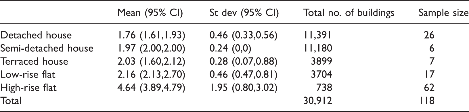
CI: confidence interval.

As can be seen from Table 1, the total number of buildings in Southampton required to validate the model stands at 118. The identification of the buildings in each sample was determined randomly by considering the 30,912 buildings in the city and utilising a MATLAB® script shown in online supplementary material. The results in Figure 2 show the distribution of the samples of each building types, their location, as well as their proximity to open spaces in the city. Furthermore, to test the statistical significance of the 118 samples, a bootstrapping test (Field et al., 2012) has been conducted using the boot package (Canty and Ripley, 2017) in statistical computing language R (version 3.4.2). The script is provided in online supplementary material. In the test, a subsample was repeatedly selected from the original sample with a total number of replications of 100,000. Results of the bootstrapping test, as shown in Table 1, give the 95% confidence interval, which agrees well with the statistic used in the sample selection. The only exception occurs in the sample of semi-detached houses, where all samples selected are found to have two floors.

Figure 2.

Location of building types for the sample size determined in Table 1 which is required to validate model estimates of building floor count.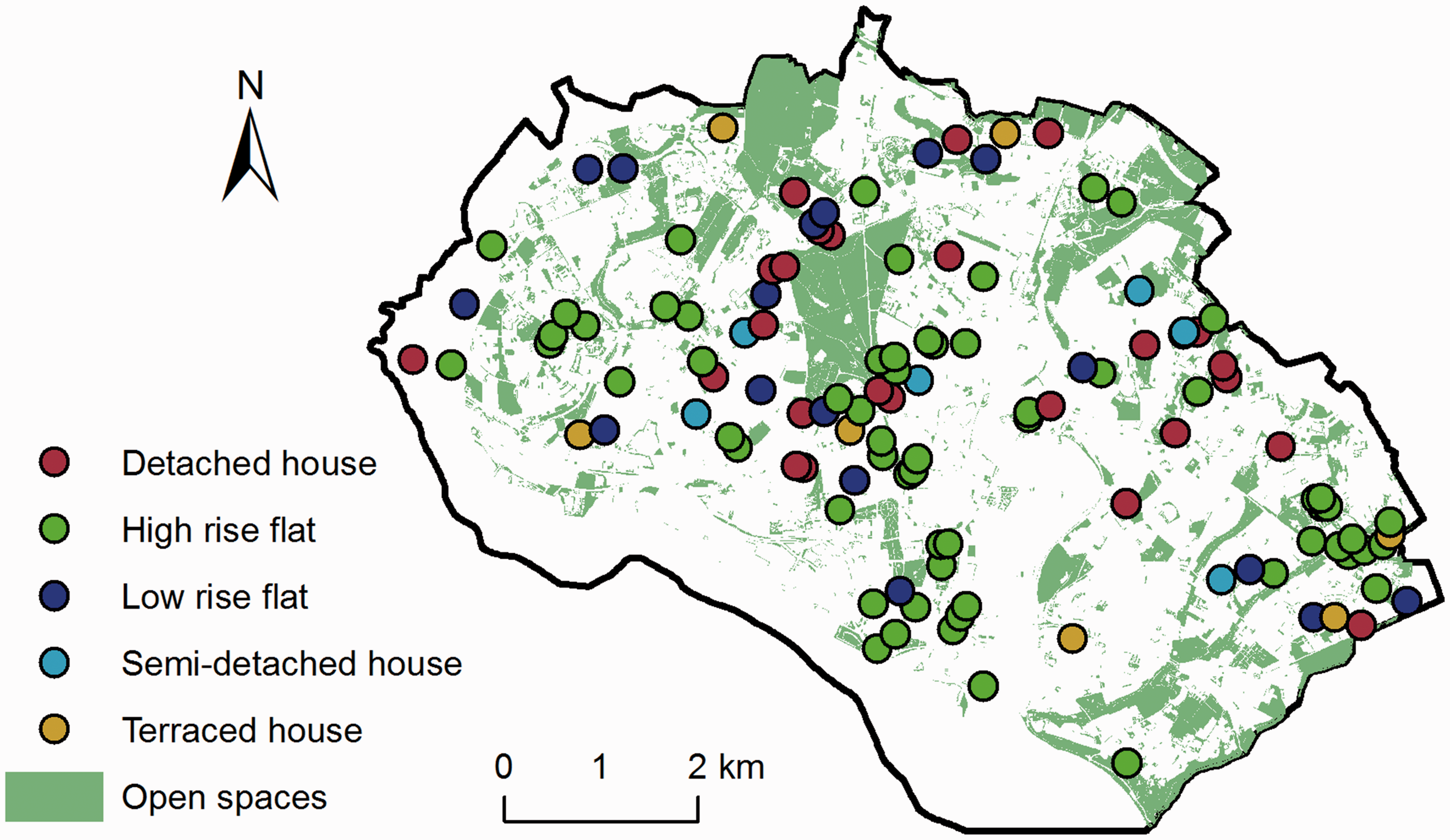

External visual surveys to determine the floor count and other features of the selected buildings were conducted in a single month in December 2014. For buildings where the floor count was difficult to judge visually during the survey, the Southampton City Council (2015) online planning portal database was used to obtain actual building information. It is important to note that the data collection procedure through the planning portal is labour intensive and time consuming, requiring manual effort to extract data from non-digital format. Conversely, visual surveys can be carried out easily and efficiently and are able to provide accurate results of the floor count of the most of the buildings. As a result, in this study visual surveys are chosen as the primary method of collecting the actual results of building floor count.

The actual floor count of the sample buildings determined from visual surveys was compared with model estimates, and the results are shown in Figure 3. As can be observed from the results, the model estimates (triangular dots) are close to the actual floor count (solid line), with a maximum error of 1.3 floors and an absolute mean error of 0.26 floors. The model estimates were also fitted to a linear correlation (dashed line in Figure 3) with an R² value of 0.95. The results are also very close with those of the actual results determined from the surveys. Nevertheless, ‘Error analysis’ section provides more details of errors analysis including observations with large residuals and a discussion on any impacts on the modelling.

Figure 3.

Comparison of the model estimates against the actual building floor counts.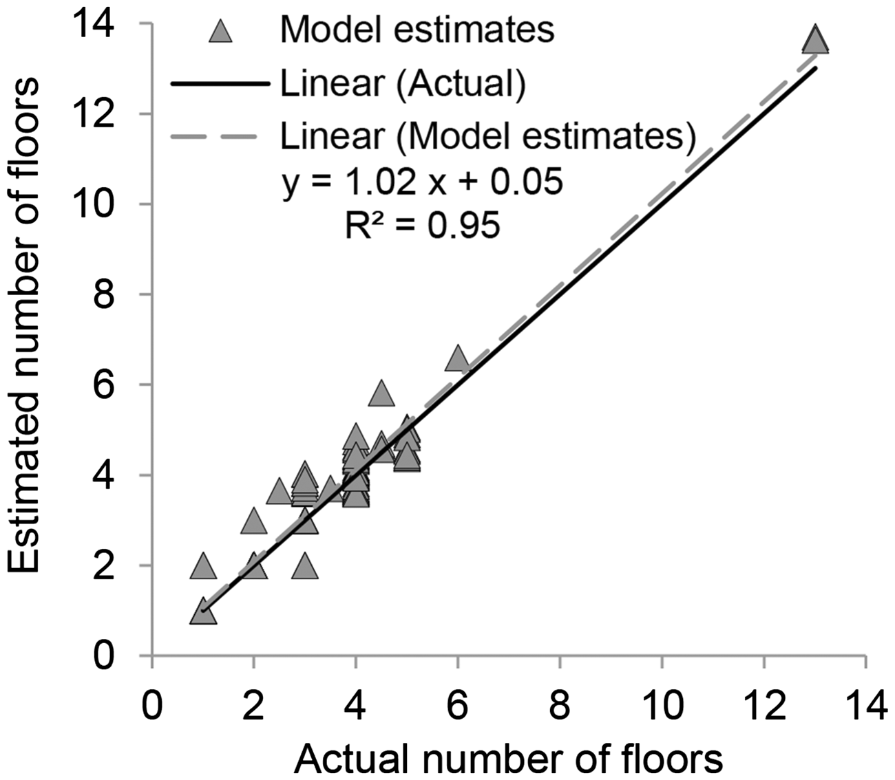

Figure 4 shows the LiDAR point occurrence densities from all the 118 sample buildings shown across different elevation bands. These include bands that have the highest/lowest elevations, the band that is identified for the principal roof part of each building, and the average results of the rest of the bands. Figure 4 also shows the results of key statistics of the analysis including max, min, median, and the range of ±1 standard deviation (σ). In this model, the first band (band of lowest elevation) is used to estimate the elevation of ground surfaces, and number of LiDAR points included in this band account for around 4.3% of the whole sample. This takes into account a fixed value of 1.2 m to enclose ground surfaces surrounding a building established in the methodology. Since the size of the 1.2 m extended areas is not comparable to the original footprint of the building, the proportion of LiDAR points in this band is relatively small compared with that in other bands.

Figure 4.

Quantity distribution of LiDAR points in various bands identified by model for each roof.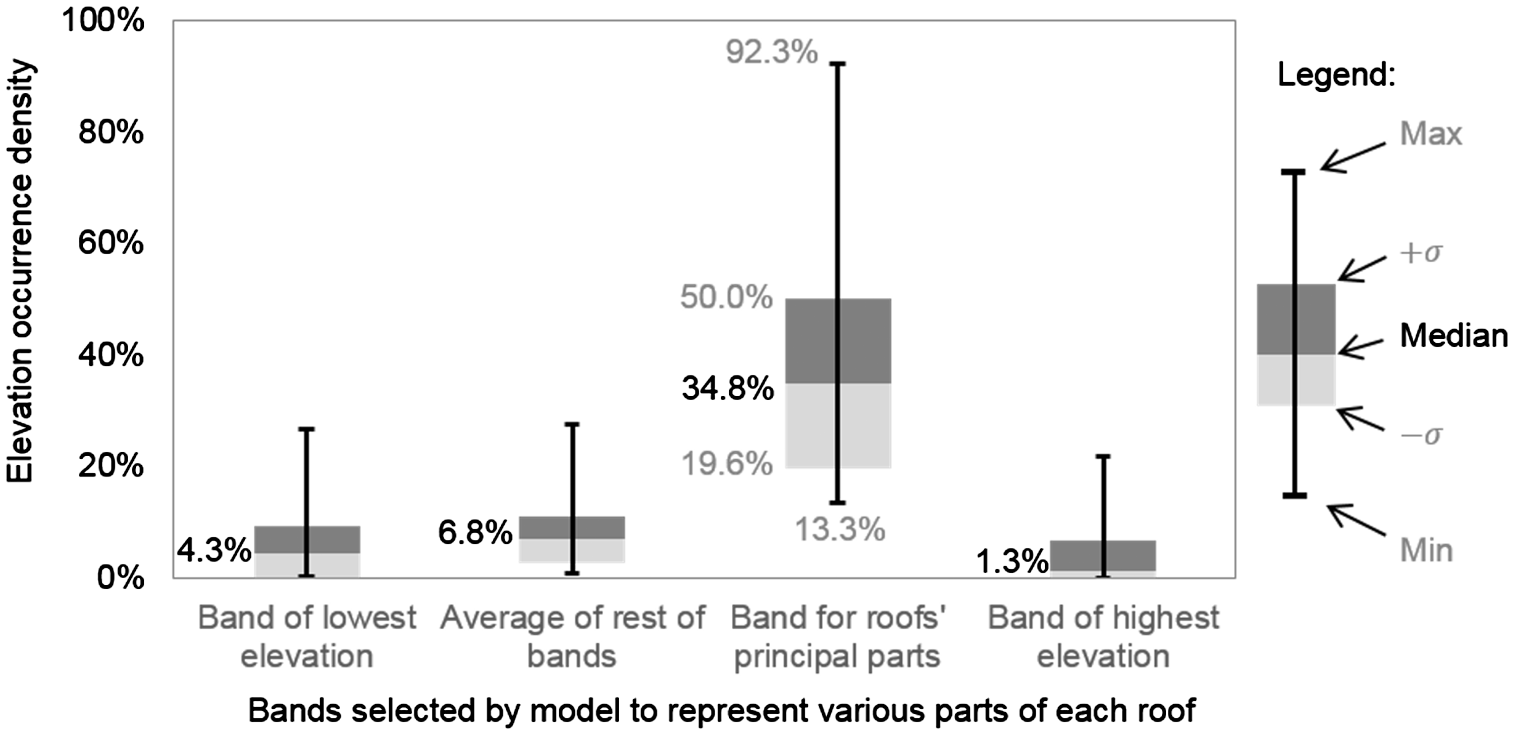

The two bands marked in the figure as the ‘roofs’ principal parts’ and ‘highest elevation’ are both for LiDAR points that are likely to be on top of a building roof, but the occurrence density (median) in the two bands varies significantly, having values of 34.8 and 1.3%, respectively. This finding agrees with the approach used in this model as the highest point on top of a roof can be affected by noise detected due to objects such as trees and chimneys, which cannot be used to represent the ceiling of living spaces underneath the roof.

Figure 4 shows that the proportion of LiDAR points falling in the principal band can vary significantly among different buildings, from 13 to over 92%. This variation is caused by differences in the structures of building roofs. For example, a flat roof would have all LiDAR points sharing the same elevation, hence a high proportion of LiDAR points in the principal band. Conversely, sloping roofs and roofs with complex structure would have a less amount of LiDAR points sharing a same band. Results of the model indicate that the lowest LiDAR point density in the roof principal band is 13%.

Buildings with multiple roof sections

Buildings in a city are likely to possess significant volumetric diversity, and the accuracy of this model on buildings of irregular shapes was tested. Figure 5 shows a building in Southampton that was initially constructed to be a four-storey block of flats but an additional floor has been added on the top of the building to serve as a penthouse accommodation (Southampton City Council Planning Portal). The penthouse, however, takes up only 50% of the roof area. This discrepancy is detected by the model, which confirms that the floor count predicted by the model is between 4 and 5, and concurs with the survey undertaken for the building (Figure 5).

Figure 5.

Sample building that has complex floor structure – block of flats with additional rooftop penthouse added to the building. Address: Balmoral Court, 16 Winn Road, Southampton, SO17 1EN.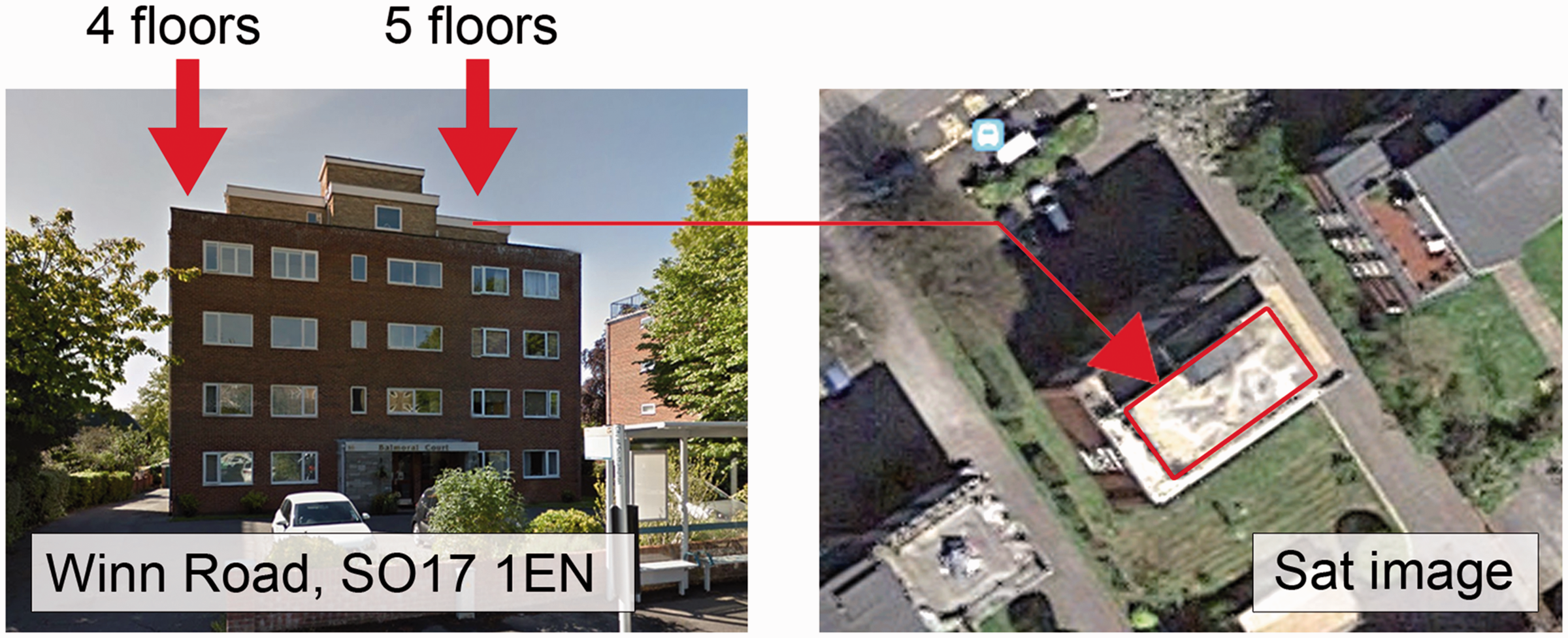

Figure 6 shows a row of terraced buildings, which have non-uniform roof structure. Buildings at the right side of the image look relatively modern and have four floors including the loft floor. On the middle of the image, buildings have three floors, whilst those on the left only have two floors. Therefore, this row of buildings has an inconsistent floor count at different sections, varying from 2 to 4. For this building block, the floor count estimated by the model is 3.70, which is within the range of the actual survey data results (i.e. a range from 2 to 4 floors). Nevertheless, as considered in equation (2) (‘Methodology’ section) and as we are addressing the building block of the whole city, this analysis is believed to cover the majority of buildings, with further discussion given in the following section.

Figure 6.

A row of terrace buildings that has varying floor counts. Address: Onslow Road, Southampton, SO14 0JD.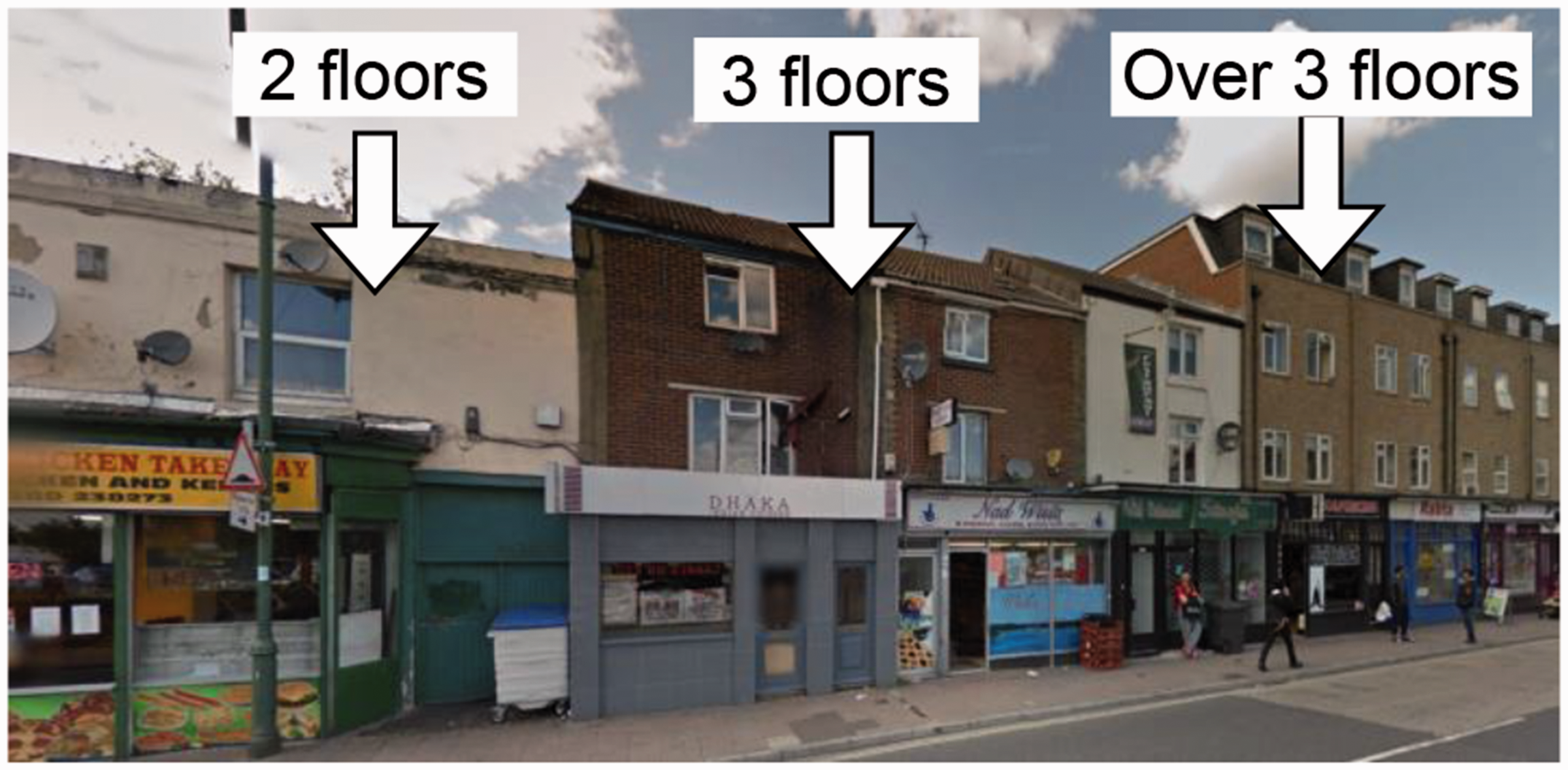

Error analysis

Error analysis was conducted to provide resilience in the model. The analysis encompasses a comparison of the model estimates with the actual building characteristics determined from visual surveys as described in ‘Sample selection and surveys’ section. The results are presented in the following sections.

Errors caused by mixed-use buildings

Figure 7 shows a building that has noticeably complex structure. Information obtained from the Southampton City Council (2015) indicated that in recent years this building has been redeveloped a number of times with frequent changes of use including semi-detached house, school, multiple occupation block of flats, hotel, and dental surgery, respectively. Currently, it is a highly mixed-use building, containing a semi-detached house on the right half (Figure 7), a dental surgery, and a residential flat on the left half. The results from the model gave an estimated floor count of 3.7 but in reality has two floors. Therefore, the abnormal building structure and the history of frequent redevelopments may have influenced the accuracy of the model when considering such buildings. Nevertheless, such cases are uncommon when considering the entire residential building stock of a city.

Figure 7.

Images of a mixed-use building which proved challenging for the model estimation of floor count. Location – Westwood Road, Southampton, SO17.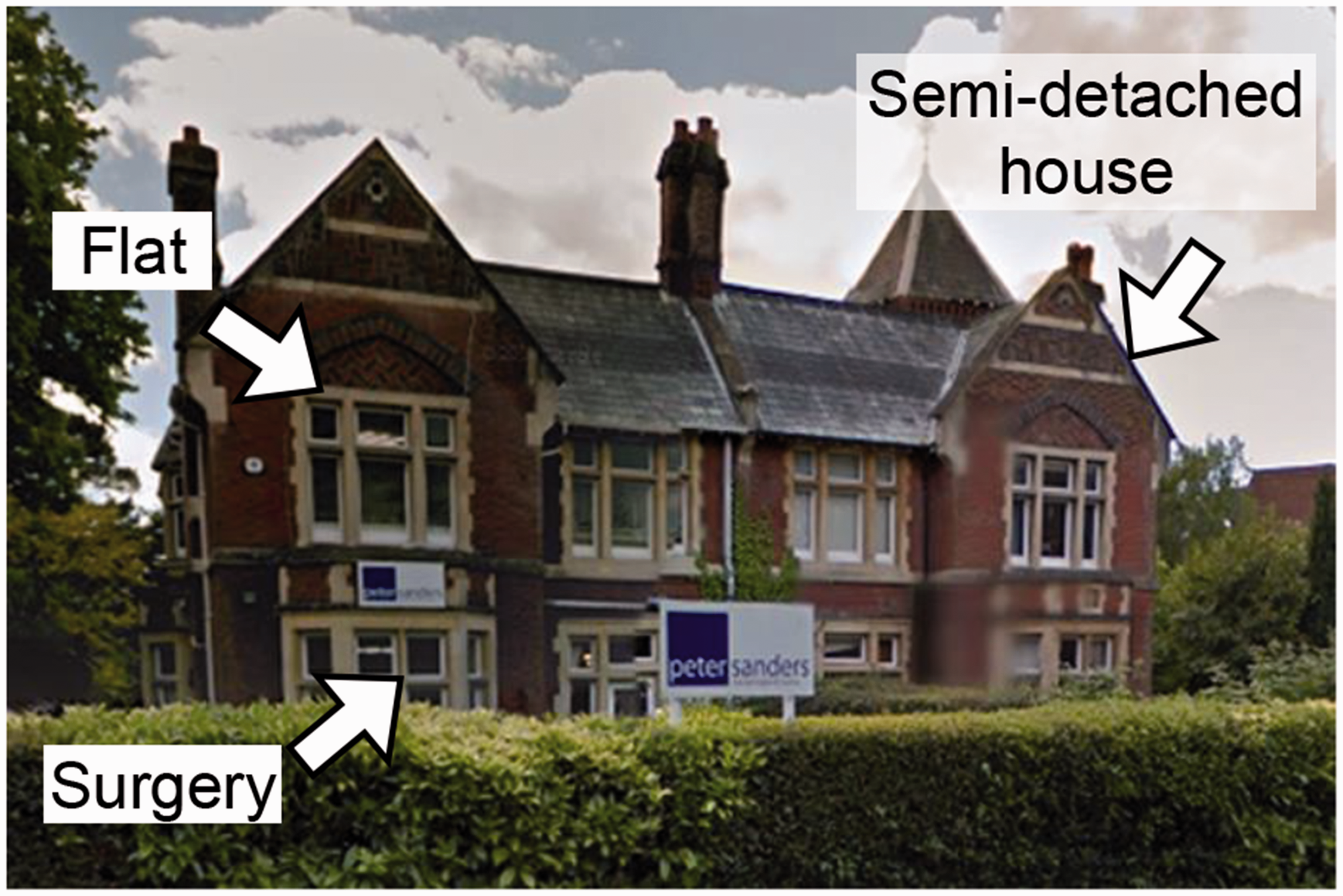

Recently in the UK, an increasing number of mixed-use buildings have been constructed as part of building redevelopment schemes, as they provide multifunctional usage of a single piece of land and are therefore more suitable for densely populated urban areas. However, currently, only a very small fraction of buildings in a city are mixed used, and they only account for 2% of the buildings in Southampton (Southampton City Council, 2012). As a result, errors caused by this group of buildings are likely to be very small when considering the overall applicability of the model over the whole city.

Errors caused by out-of-date data

Figure 8 shows a series of images of the same building from various data sources. The building occupies a total ground area of almost 1000 m². Up to 2011, this site was used to accommodate 73 flats. Part of the building was then demolished and redeveloped and now consists of a three-storey building providing 34 flats for the elderly. Such redevelopment has not been updated by the OS Building MasterMap®, obtained on September 2014. As shown in Figure 8(a), building outlines drawn by OS have the same shape of buildings shown in the satellite image dated 2004 (Figure 8(b)), but the outlines show significant discrepancy with the 2015 satellite image (Figure 8(c)). It is clear that the left (west) half of the construction was built with sloping roofs, whereas the previous had a single piece of flat roof. In the OS dataset, however, the two parts of the building site have been linked together, and the outlines have been merged into a single polygon. As a result, the height difference between the two parts of the building has not been recognised by the model, hence an estimation error. Clearly, the output of the model will rely significantly on the input data, hence care is needed to check such datasets and update them accordingly.

Figure 8.

Variation in data availability where the images show a building complex that was not updated on OS building MasterMap® as compared with recent data. (a) OS building outline, (b) Satellite image (2004), and (c) Satellite image (2015, Google).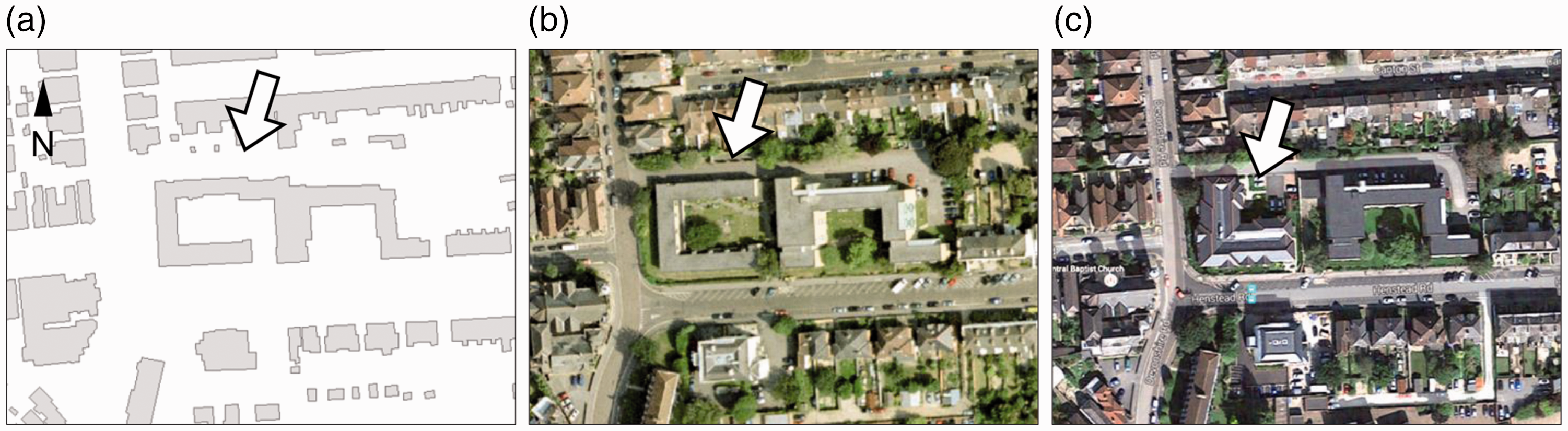

Comparison with OS building height dataset

Since 2015, the OS has released a series of datasets of estimated height of individual buildings using its own developed model (hereinafter referred to as the ‘OS dataset’). In this section, results from the OS dataset (beta version, which is the latest version released in February 2018) were compared with estimates from the presented model. The comparisons are aimed at testing the ability of the two models to provide an accurate estimate of the floor count in a building. The estimates of building heights provided by OS dataset and the model were first converted into estimates of building floor count using the same algorithm (see ‘Methodology’ section). These results were then compared with the actual floor counts obtained from visual surveys conducted on the sample buildings discussed in ‘Results and analysis’ section. The comparison results are presented in Table 2. It shows that both results are close to the actual floor counts of buildings. The mean absolute error of the presented model is 0.26, which is 23% smaller than that of the OS data (0.32). Furthermore, the OS data also have a greater maximum error, three floors, compared with that of the presented model, which is only 1.32 floors. Both results have a similar proportion of errors that are under ±0.5 floors, which are 79% from the presented model versus 74% by the OS dataset.

Table 2.

Errors in the estimates of building floor count: present model versus OS dataset.

	Mean abs. error	Max abs. error	Percentage of errors under ±0.5 floors
Model here by presented	0.26	1.32	79
OS dataset	0.32	3.00	74

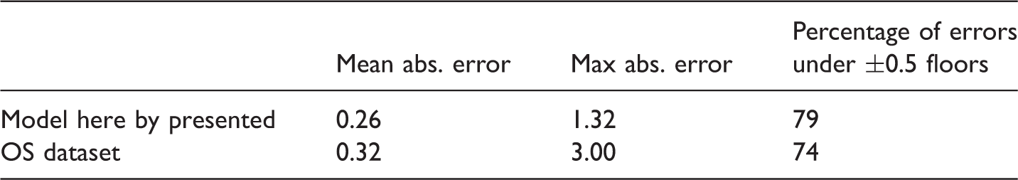
OS: Ordnance Survey.

Conclusions

This work presents a new modelling approach to estimate the height and floor count of individual buildings at city scale. LiDAR data were used to identify the principal part of a building roof and the ground surface in close proximity to the building. The elevation of these two positions was used to estimate the net height and the floor count of a building under consideration. This approach avoids errors that can be caused by objects such as those installed on top of buildings and by the interpolation procedure for estimating the elevation of ground surface. The accuracy of the developed model was validated using actual data obtained from visual observation of a number of randomly selected buildings in Southampton. The results obtained for the estimated floor count of a building have a mean absolute error of 0.26 floors, with the maximum error of 1.32 floors. All of the computations were conducted on a consumer-level PC with an Intel(R) Core(TM) i7-2600 3.4 GHz CPU, 16 GB RAM, running the Windows 7 64-bit operating system. The average time for the floor count estimation was 0.24 s per building, and the test on all buildings in Southampton (n = 30,912) was completed within 124 minutes.

The approach and the model described in this paper address a current gap in knowledge reported numerous times in the literature as an obstacle for conducting building-level simulations (González-Aguilera et al., 2013; Orford, 2010). The model provides an automatic estimation of building height or floor count conducted in a GIS platform. The information provided by the model, especially at a city scale is crucial as it provides internal volume of a building which is needed for determining the energy demand, property price, level of wellbeing, and a number of socio-economic factors.

Supplemental Material

Appendices -Supplemental material for City-wide building height determination using light detection and ranging data

Supplemental material, Appendices for City-wide building height determination using light detection and ranging data by Yue Wu, Luke S Blunden and AbuBakr S Bahaj in Environment and Planning B: Urban Analytics and City Science

Footnotes

Acknowledgements

This work is part of the activities of the Energy and Climate Change Division and the Sustainable Energy Research Group at the University of Southampton (). The authors would also acknowledge Southampton City Council for providing citywide data.

Declaration of conflicting interests

The author(s) declared no potential conflicts of interest with respect to the research, authorship, and/or publication of this article.

Funding

The author(s) disclosed receipt of the following financial support for the research, authorship, and/or publication of this article: This work is supported by EPSRC under grants: City-Wide Analysis to Propel Cities towards Resource Efficiency and Better Wellbeing (EP/N010779/1), Transforming the Engineering of Cities to Deliver Societal and Planetary Wellbeing (EP/J017698/1), and International Centre for Infrastructure Futures (EP/K012347/1).

Yue Wu is a researcher in sustainable energy within the Energy and Climate Change Division at the University of Southampton. His research interest includes city-scale energy modelling, carbon reduction, and sustainable development. He is currently working on a number of city-scale research projects aiming at improving citizen’s wellbeing while reducing the carbon emissions from the use of domestic and non-domestic energy.

Luke S Blunden is researcher in Sustainable Energy within Engineering and the Environment at the University of Southampton. His research interest includes marine renewable energy resources, energy for development, and sustainability of cities. He is currently working on a number of city-scale research projects aiming at improving citizen’s wellbeing while reducing the carbon emissions from the use of domestic and non-domestic energy.

AbuBakr S Bahaj (FICE, FRSA, MInstP, CPhys) leads the 55-strong Energy and Climate Change Division at the University of Southampton, where he completed his PhD, progressing from a researcher to a Personal Chair in Sustainable Energy. For more than 25 years, Bahaj has pioneered sustainable energy research and established the energy theme within the University. His major research programmes can be found at . These include Cities and Infrastructure, Data and Modelling, Energy and Behaviour, Energy and Buildings, Energy for Development, Environmental Impacts, Microgeneration Technologies, and Renewable Energy (Solar Photovoltaics and Marine Energy).

References

Abellán

Moral

(2003) Building classification trees using the total uncertainty criterion. International Journal of Intelligent Systems 18(12): 1215–1225.

Amini H, Pahlavani P and Karimi R (2014) 3D reconstruction of buildings with gabled and hipped structures using LiDAR data. In: ISPRS – International Archives of the Photogrammetry, Remote Sensing and Spatial Information Sciences XL-2/W3, November, pp.47–52.

Arefi

Reinartz

(2013) Building reconstruction using DSM and orthorectified images. Remote Sensing 5(4): 1681–1703.

Balaras

, et al. (2005) Heating energy consumption and resulting environmental impact of European apartment buildings. Energy and Buildings 37(5): 429–442.

Canty A and Ripley B (2017) boot: Bootstrap R (S-Plus) functions. R package version 1.3-20.

Chen

, et al. (2012) Upward-fusion urban DTM generating method using airborne Lidar data. ISPRS Journal of Photogrammetry and Remote Sensing 72: 121–130.

Department for Communities and Local Government (2017) Energy performance of buildings data: England and Wales. Available at: https://epc.opendatacommunities.org/ (accessed 21 July 2017).

Environment Agency (2013) LIDAR composite DSM. Available at: http://www.environment-agency.gov.uk/default.aspx (accessed 21 July 2017).

Field AP, et al. (2012) Discovering statistics using R. London, SAGE.

10.

Galvanin EADS Dal Poz

(2011) Extraction of building roof contours from LiDAR data using a Markov-random-field-based approach. IEEE Transactions on Geoscience and Remote Sensing 50(3): 981–987.

11.

Geoinformation Group (2014) UK buildings: Property insights through smarter data. Available at: http://www.geoinformationgroup.co.uk/#!ukbuildings/c1his (accessed 21 July 2017).

12.

González-Aguilera

, et al. (2013) Automated urban analysis based on LiDAR-derived building models. IEEE Transactions on Geoscience and Remote Sensing 51(3): 1844–1851.

13.

Gupta R and Gregg M (2014) Using urban energy modelling to rapidly assess potential for climate change mitigation and adaptation of UK homes. In: Building simulation and optimization BSO14.

14.

Hong

Oreszczyn

Ridley

(2006) The impact of energy efficient refurbishment on the space heating fuel consumption in English dwellings. Energy and Buildings 38(10): 1171–1181.

15.

Huang

, et al. (2017) A novel building type classification scheme based on integrated LiDAR and high-resolution images. Remote Sensing 9(7): 679.

16.

Iannelli

Dell’Acqua

(2017) Extensive exposure mapping in urban areas through deep analysis of street-level pictures for floor count determination. Urban Science 1(2): 16.

17.

Iowerth H, et al. (2013) A SAP sensitivity tool and GIS-based urban scale domestic energy use model. In: Proceedings of BS2013, pp. 452–459.

18.

Jaggs

Palmer

(2000) Energy performance indoor environmental quality retrofit – A European diagnosis and decision making method for building refurbishment. Energy and Buildings 31(2): 97–101.

19.

Kreyszig E (2011) Advanced Engineering Mathematics. Hoboken, NJ, John Wiley.

20.

Guan

(2011) 3D building reconstruction from airborne lidar point clouds fused with aerial imagery. In: Yang

(ed.) Urban Remote Sensing: Monitoring, Synthesis and Modeling in the Urban Environment, Chichester: John Wiley & Sons, Ltd, pp. 75–91.

21.

Liang-Chien C, Tee-Ann T, Rau JY, et al. (2005) Building reconstruction from LIDAR data and aerial imagery. In: Proceedings. 2005 IEEE International Geoscience and Remote Sensing Symposium, 2005. IGARSS '05., pp. 2846–2849.

22.

Liang

Shen

(2012) Determining sample size for building energy consumption surveys using statistical theory. Energy and Buildings 47(1): 533–539.

23.

Meng

Currit

Zhao

(2010) Ground filtering algorithms for airborne LiDAR data: A review of critical issues. Remote Sensing 2(3): 833–860.

24.

Office for National Statistics; National Records of Scotland; Northern Ireland Statistics and Research Agency (2016): 2011 Census aggregate data. UK Data Service (Edition: June 2016). DOI: http://dx.doi.org/10.5257/census/aggregate-2011-1.

25.

Ordnance Survey (2014) OS MasterMap. Available at: http://digimap.edina.ac.uk/digimap/home (accessed 21 July 2017).

26.

Orford

(2010) Towards a data-rich infrastructure for housing-market research: Deriving floor-area estimates for individual properties from secondary data sources. Environment and Planning B: Planning and Design 37(2): 248–264.

27.

Reinhart

Cerezo Davila

(2016) Urban building energy modeling – A review of a nascent field. Building and Environment 97: 196–202.

28.

Rottensteiner

(2003) Automatic generation of high-quality building models from LiDAR data. IEEE Computer Graphics and Applications 23(6): 42–50.

29.

Rottensteiner

Briese

(2002) A new method for building extraction in urban areas from high-resolution LIDAR data. International Archives of Photogrammetry and Remote Sensing 34(3): 295–301.

30.

Sampath A and Shan J (2010) Segmentation and Reconstruction of Polyhedral Building Roofs From Aerial Lidar Point Clouds, In: IEEE Transactions on Geoscience and Remote Sensing 48(3): 1554–1567.

31.

Siddiqui FU, et al. (2013) An improved building detection in complex sites using the LIDAR height variation and point density. In: International conference image and vision computing, New Zealand, pp.471–476.

32.

Southampton City Council (2015) Southampton city council planning applications and decisions public portal. Available at: https://planningpublicaccess.southampton.gov.uk/online-applications/ (accessed 1 August 2017).

33.

Tobergte

Curtis

(2013) Spatial autoregressive model for population estimation at the census block level using LIDAR-derived building volume information fang. Journal of Chemical Information and Modeling 53(9): 1689–1699.

34.

Truong-Hong

Laefer

(2015) Quantitative evaluation strategies for urban 3D model generation from remote sensing data. Computers & Graphics 49: 82–91.

35.

, et al. (2017a) A graph-based approach for 3d building model reconstruction from airborne LiDAR point clouds. Remote Sensing 9(1): 92.

36.

, et al. (2017b) An extended minimum spanning tree method for characterizing local urban patterns. International Journal of Geographical Information Science 32(3): 1–26.

37.

Yan

, et al. (2016) Phase analysis of three-dimensional Zernike moment for building classification and orientation in digital surface model. IEEE Geoscience and Remote Sensing Letters 13(1): 58–62.

38.

, et al. (2010) Automated derivation of urban building density information using airborne LiDAR data and object-based method. Landscape and Urban Planning 98(3–4): 210–219.

39.

Zheng

Weng

Zheng

(2017) A hybrid approach for three-dimensional building reconstruction in Indianapolis from LiDAR data. Remote Sensing 9(4): 310.

Supplementary Material

Please find the following supplemental material available below.

For Open Access articles published under a Creative Commons License, all supplemental material carries the same license as the article it is associated with.

For non-Open Access articles published, all supplemental material carries a non-exclusive license, and permission requests for re-use of supplemental material or any part of supplemental material shall be sent directly to the copyright owner as specified in the copyright notice associated with the article.

0.00 MB

0.87 MB