Sage Journals: Discover world-class research

Abstract

Location and accessibility are core concepts for land-value research. However, the perspective is still limited in their conceptual and methodological application to cities from the Global South. The objective of this research is to bridge concepts and definitions to comprehensively operationalize accessibility indicators and uncover its relation with residential land-values in Guatemala City. We developed a multivariate regression model using the following access metrics: (1) geographic-access indices that were computed using time-based analyses per transport mode; (2) geometric-access metrics estimated via Space Syntax at various spatial scales; (3) a proposed geometric via geographic-access metric computed as potential access to network centrality. A variable selection process allowed to assess the information contribution of each variable in building a parsimonious model. We assessed the model in the context of model variations that represent common approaches used in existing literature. Geographic access to the core business district has the highest impact on the land-values, followed by proximity to urban areas with high geometric-access, measured as geometric via geographic access. Geometric accessibility at neighbourhood and city-wide scales add spatialized information that contributes to a parsimonious model and reduces spatial dependence. The model yielded the highest goodness of fit and prediction accuracy compared with the model variations. We concluded that Guatemala City land-values follow a predominant monocentric structure. Additionally, potential access to vital urban areas as identified via Space Syntax denotes the presence of economic activities, or potential for such, which were not explicitly addressed through the geographic-access metrics. The results have limitations but pose methodological possibilities relevant for research and practice in similar Latin American cities.

Keywords

Land-value Space Syntax accessibility multivariate regression Guatemala

Introduction

Following Krause and Bitter (2012), trends in land and property value research can be grouped in three. First, uncovering the relation between the various factors that can influence the value formation is commonly done using hedonic pricing, and implemented through multivariate linear regression techniques (Liu et al., 2010; Munroe, 2007). However, there is a growing body of literature concerned with the presence of spatial dependence and the statistical methodological expansions to address it, such as spatial econometrics (Bourassa et al., 2007; Lesage and Pace, 2009). Second, literature is placing attention on studying the value of land after recognizing differences between this value and the value of the improvements (i.e. construction). Land is fixed both in territorial location and its supply (Evans, 1987), which could make it more volatile and sensitive to the effects of demand, location and economic shocks (Krause and Bitter, 2012). Third, interest is taking place on studying the value effects derived from sustainable urban processes such as mixed-uses, mass transport and street connectivity (Anantsuksomsri and Tontisirin, 2015; Matthews and Turnbull, 2007). It can be said that this has always been central in this research area, but only implicitly by means of the urban accessibility concept (Adair et al., 2000; Ahlfeldt, 2007; Des Rosiers et al., 2000; Giuliano et al., 2010; Liu et al., 2010).

Location and accessibility are core concepts in land-value and house-price research (Orford, 2002; Webster, 2010). Important urban economic theories (Alonso, 1964; Evans, 1987; Muth, 1969) and a large body of literature prove that relative location and access externalities are associated with the economic value of various land-uses (Dale-Johnson and Brzeski, 2001; Evans, 1987; Kivell, 1993; Liu et al., 2010; Peiser, 1987). Basic accessibility concepts and methods have been commonly at the core of previous research on land-value modelling, particularly in urban areas (Iacono and Levinson, 2011; Saeid, 2011). However, cities are no simple phenomena and there is still room for exploring their application, particularly in cities from the Global South.

We address location using two types of accessibility. Geographic-accessibility reflects the easiness to reach a location or to be reached given available infrastructure to overcome impedance between origin and destination (Batty, 2009). Distance, travel-time, cumulative opportunities and gravity-type measurements are metrics commonly used in research and practice (Geurs and Van Eck, 2001). In turn, Geometric-accessibility is defined as a resource given the topologic-geometric characteristics of a city urban layout (Jiang et al., 1999; Webster, 2010). Network-closeness and network-betweenness are common network centrality metrics that are associated with geometric-accessibility (Freeman, 1977; Porta et al., 2005). Space Syntax (SSx) is a set of theories and methods based on graph theory and dual representations of the urban layouts that is pioneer in network centrality applied to urban areas (Bafna, 2003; Hillier et al., 2012; Webster, 2010). Integration and choice are SSx metrics, adopted in this research, equivalent to closeness and betweenness correspondingly.

The trade-off neoclassic theory (Alonso, 1964; Evans, 1987) constitutes a fundamental basis for land-value and house-price literature (Ahlfeldt and Wendland, 2011; Kivell, 1993). Accessibility is then mainly addressed as proximity to a core business district (CBD) and other location externalities. Proximity measurements are commonly included as aerial or network-based distances (Bourassa et al., 2007; Dale-Johnson and Brzeski, 2001; Heikkila et al., 1989; Liu et al., 2010; Munroe, 2007; Orford, 2002; Waddell et al., 1993). Metric distances are not realistic measurements as road characteristics and transport modes pose different travel times or costs over the same distance (Mavoa et al., 2012; Ryan, 1999). Some literature used travel-times instead (Ahlfeldt and Wendland, 2011; Iacono and Levinson, 2015; Ottensmann et al., 2008; Pujol et al., 2013). However, the focus has mostly been placed on travel times by private mobility. Relatively few research has tested more complex methods such as the potential measurements to replace the traditional CBD proximity (Adair et al., 2000; Ahlfeldt, 2007; Du and Mulley, 2012; Giuliano et al., 2010; Osland and Thorsen, 2013). The rationale is that a monocentric CBD assumption might not adequately capture access to economic opportunities due to emergence of polycentric structures.

The availability of public transport is mostly addressed as proximity to access points (i.e. stops and stations) to such infrastructure (Ryan, 1999) (e.g. Anantsuksomsri and Tontisirin, 2015; Iacono and Levinson, 2011; Ibeas et al., 2012; Rodríguez and Mojica, 2009; Waddell et al., 1993). Such approach is commonly used to sort out the effects of public transport investments on house-value properties, again assuming mono-centricity (Ryan, 1999). Only very limited research has used simultaneously travel-times measurements by more than one transport mode (Adair et al., 2000; Des Rosiers et al., 2000; Du and Mulley, 2012). Adair et al. (2000) used travel times per transport mode and estimated mean access values for each neighbourhood in its study area.

Only a small body of literature has addressed geometric accessibility combined with basic geographic access metrics. Desyllas (1997) investigated the relationships between the evolution of land-use and geometric-access with land-values in Berlin. Matthews and Turnbull (2007) investigated the effects of integration and proximities to selected land-uses on house-prices in Washington. Enström and Netzell (2008) investigated the effects of integration on office-rent variation in downtown Stockholm. Chiaradia et al. (2009) researched on the associations between geometric access and dwellings values in London. Saeid (2011) analysed the relation between integration with land-values in Wroclaw. Xiao et al. (2016) studied various spatial scales at where geometric-accessibility, together with selected geographic-access metrics, better explains house-price variability in Cardiff.

Overall, the outcomes of these works provide evidence on how geometric access can explain land-values more accurately. SSx metrics at various spatial scales provide additional information about the quality of the urban layout that other access metrics cannot capture. Furthermore, these metrics could have the potential to improve the quality of the model itself in terms of reducing heteroskedasticity and spatial autocorrelation (Xiao et al., 2016). SSx methodologies have evolved and developed in more sophisticated analyses compared to the early applications (Steadman, 2004; Turner, 2007), but only limited research have implemented along newer techniques in land-value investigations (Chiaradia et al., 2009; Xiao et al., 2016). Additionally, these works are mostly limited to case studies from developed and planned cities.

We define the research gap as the need of bridging available concepts and methods in the field of accessibility studies with the land-value modelling task. We introduce the following hypotheses. (1) Addressing the disparity of geographic-access opportunities due to available transport modes and the geometric-access at various spatial scales could contribute to an increased capacity to explain land-values variability and prediction accuracy. (2) Geometric-accessibility capitalizes land not only at location, but also as a reachable resource by means of geographic-access. Thus, geometric via geographic accessibility is defined as the easiness to reach geometric access by means of private or public transport-based mobility. Such metrics could reflect access to urban areas with presence of facilities or economic activities (or a potential for such), which are not explicitly addressed in other geographic-access metrics.

The objective of this research is to bridge concepts and definitions to comprehensively operationalize accessibility indicators and uncover its relation with residential land-values in Guatemala City. We developed one multivariate regression model that used the following access metrics: (1) geographic access indexes that were computed using time-based analyses per transport mode; (2) geometric access metrics estimated via SSx at various spatial scales; (3) a proposed geometric via geographic access metric computed as a potential access to network centrality as analysed in SSx. A parsimonious model is estimated following a variable selection procedure and then assessed using various performance statistics.

The remainder of this paper is organized as follows. Materials and methods introduce the study area, data pre-processing and methods. Then, the results are presented and discussed. Here, we interpret the impacts of the various access metrics on the value of residential land, as well as the performance of the model. Finally, we address the conclusions where we reflect on the limitations and implications of the results in further research and practice.

Materials and methods

Case study

Our case study city is Guatemala City, Guatemala. Similar to other Latin American cities with colonial origins, Guatemala’s historic centre has a gridiron urban structure (Gellert, 1990; Pacione, 2005: 447–602). First expansions by the end of 1800s and up to middle 1900s were carried out by local planners. Later, a combination of socio-political conditions, natural events and a massive migration from rural areas resulted in unplanned expansion towards the periphery. A CBD of white collars emerged towards the south of, and linked to, the historic core following important infrastructure such as the inter-American road (CA-1) and the international airport (Figure 1). Jobs and important economic activities are highly centralized there, whilst population density tends to show a decentralized pattern (DPU, 2009). The case study is relevant for the region as various Latin American cities display similar city structure and dynamics (Ford, 1996; Ingram and Carroll, 1981).

Figure 1.

Appraisals location (top), and land-value frequency distributions before and after transformation (bottom).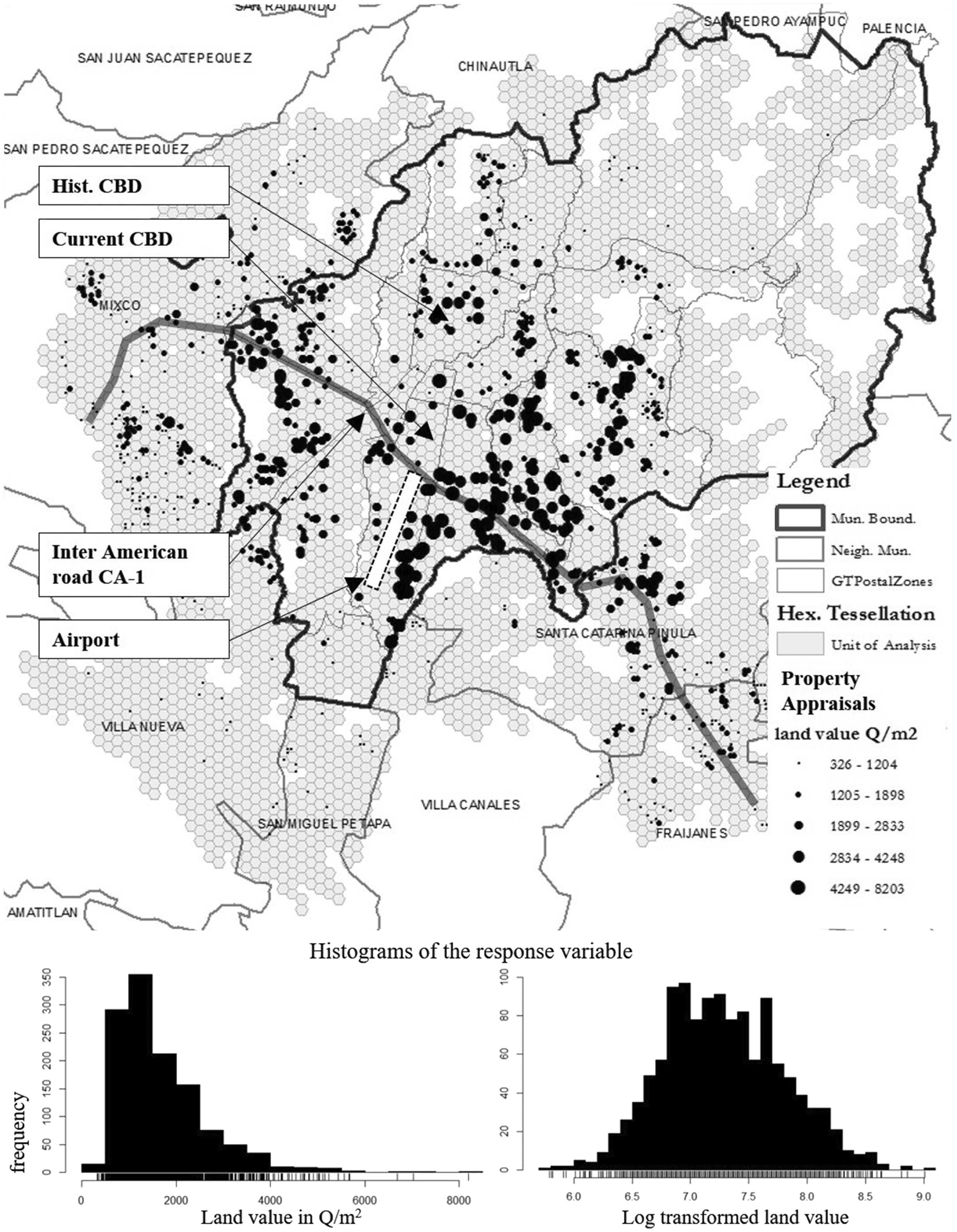

Data pre-processing, variables and descriptive statistics

Land-value data were collected during fieldwork (August 2014–April 2015). We built a spatial database indexing 2000 records of real-estate property appraisals (observations) dating from the years 2008–2014, and carried out by a Guatemalan private office (AO). Observations were geo-referenced to the centroid of each property using the WGS84 co-ordinate system (Decker, 1986). According to the AO, the observations report “arm-length values” reflecting optimum transaction values where there is no pressure to sell or buy, and parties have complete information. Land-values are in local currency Quetzal (Q) per square meter of plot surface area. These were deflated to the year 2014 using the Guatemalan consumer price indexes (Ine, 2016), and transformed to natural logarithms to deal with a non-normal distribution and potential non-linear relations with the predictors. We only used observations of residential uses (excluding flats) and plots with surface areas between 100 and 1000 m². Figure 1 shows the location of the 1026 observations used in this research.

Accessibility metrics were mostly produced in previous work and are aggregated in a hexagonal tessellation (Morales et al., 2016). The size of the hexagons (300 m inner-diameter) provided an adequate resolution at an affordable computational demand. Geographic access metrics were available per transport mode. Additional variables, further described, were also mapped and aggregated to this tessellation (except property-level characteristics). Where one hexagon contained more than one observation, same predictor values were attached to the observations.

Table 1 shows descriptive statistics of the land-values and the predictors included in our model. Geographic accessibility metrics addressed location externalities that are assumed and empirically proven to influence residential markets in existing property-value literature (Des Rosiers et al., 2000; Du and Mulley, 2012; Liu et al., 2010). According to local experts, access to these externalities is relevant to define location quality (Morales et al., 2016). Access to neighbourhood-scale groceries, banks and restaurants, parks, schools, clinics and open markets were assumed to benefit a location within limited time radii and are of an “optional nature”, meaning that users appreciate close proximity and amount of available options. Thus, access to those was measured as a cumulative opportunity within a 10-minute travel time (Morales et al., 2016). We assumed that a cumulative measurement would capture the benefit from accessible concentrations of such facilities, compared to the shortest travel-time to one of the facilities.

Table 1.

List of variables and descriptive statistics.

Group	Acronym	Description	Type	Mean	St. Deviation	Min	Max	% coded 0	% coded 1
Response variable	lv	Land value in Q/m²	Ratio	1678.45	958.41	325.75	8203.43	□	□
Geographic accessibility by public transport	stand_groceries	Standardized access score (from 0 to 1) based on number of facilities accessible within 10 minutes driving	Ratio	0.08	0.14	0.00	0.80	□	□
	stand_bank_rest			0.04	0.09	0.00	0.94	□	□
	stand_parks			0.05	0.09	0.00	0.76	□	□
	stand_schools			0.03	0.10	0.00	1.00	□	□
	stand_clinics			0.06	0.13	0.00	1.00	□	□
	stand_markets			0.03	0.13	0.00	1.00	□	□
	time_cbd	Travel time to CBD	Ratio	27.21	9.74	2.13	51.59	□	□
	time_jobs	Gravity-based access to job opportunities		116,375	50,122	1244	240,368	□	□
	time_xl_mall	Travel time to closest facility using public transport		39.50	18.56	3.00	109.00	□	□
	time_xl_grocery			29.08	15.26	2.00	93.00	□	□
	time_university			39.86	22.89	2.00	130.00	□	□
	time_culture			42.44	21.23	2.00	111.00	□	□
	time_hospital			30.90	19.11	0.00	101.00	□	□
	time_xl_sports			50.20	24.12	4.00	136.00	□	□
Geographic accessibility by private vehicle	s_groceries	Standardized access score (from 0 to 1) based on number of facilities accessible within 10 minutes driving	Ratio	0.24	0.20	0.00	0.91	□	□
	s_ban_rest			0.10	0.16	0.00	0.99	□	□
	s_parks			0.13	0.19	0.00	1.00	□	□
	s_schools			0.12	0.18	0.00	1.00	□	□
	s_clinics			0.17	0.21	0.00	0.95	□	□
	s_markets			0.10	0.18	0.00	1.00	□	□
	time_cbd	Travel time to CBD using private vehicle	Ratio	59.72	20.92	8.70	127.80	□	□
	time_jobs	Gravity-based access to job opportunities		48,502	20,746	9964	96,362	□	□
	time_xl_mall	Driving time to closest facility		14.60	6.42	0.00	33.00	□	□
	time_xl_grocery			11.36	6.47	1.00	33.00	□	□
	time_university			17.02	9.65	1.00	48.00	□	□
	time_culture			19.26	9.69	0.00	42.00	□	□
	time_hospital			12.56	8.24	0.00	41.00	□	□
	time_xl_sports			21.48	9.87	1.00	51.00	□	□
Geometric accessibility (Space Syntax)	int_08	Average integration r_0.8Km	Ratio	49.95	35.86	6.37	272.05	□	□
	int_15	Average integration r_1.5Km		106.21	90.15	6.33	558.83	□	□
	int_25	Average integration r_2.5Km		206.21	191.25	8.80	1060.01	□	□
	int_50	Average integration r_5Km		524.75	475.18	58.28	2399.83	□	□
	int_75	Average integration r_7.5Km		922.39	754.09	135.55	3244.11	□	□
	int_n (global)	Average integration r_N		3063.56	863.52	1396.33	4807.18	□	□
	nach_08	Max. normalized choice r_0.8Km		1.26	0.18	0.00	1.56	□	□
	nach_15	Max. normalized choice r_1.5Km		1.23	0.18	0.00	1.53	□	□
	nach_25	Max. normalized choice r_2.5Km		1.21	0.18	0.00	1.44	□	□
	nach_50	Max. normalized choice r_5Km		1.16	0.18	0.00	1.43	□	□
	nach_75	Max. normalized choice r_7.5Km		1.14	0.19	0.00	1.44	□	□
	nach_n	Max. normalized choice r_N		1.10	0.19	0.00	1.49	□	□
Proximity to infrastructure	dist_mroad	Planar distance to main roads as classified in OSM, expressed in meters	Ratio	333.11	313.19	0.19	1492.12	□	□
Proximity to infrastructure	dum_prox_bus	1 if location is within 500mt distance to any bus line	Dummy	□	□	0	1	33%	67%
Submarkets	dum_west	1 if area is within the west municipalities	Dummy	□	□	0	1	78%	22%
	dum_east	1 if area is within the east municipalities	Dummy	□	□	0	1	84%	16%
	condo_seg	Average total selling price of horizontal housing offer classified from 0 to 3 accord.	Ratio	1.83	1.11	0.00	3.00	□	□
	flat_seg	Average total selling price of vertical housing offer classified from 0 to 3 accord.	Ratio	0.84	1.07	0.00	3.00	□	□
Neighbourhood characteristics	pop_dens	Population density projected to 2015*	Ratio	46.83	21.62	3.38	98.26	□	□
	soc_economic	Predominant socio economic level (from 1 to 5) per census block		4.28	0.97	1.00	5.00	□	□
	percent_priv	Percentage of private-vehicle-based generated trips per TAZ		0.22	0.18	0.03	0.89	□	□
	dens_flats	Density of recent horizontal housing offer (2013–2014) expressed in units/km²	Ratio	4785.69	7024.00	0.00	36605.64	□	□
	dens_condos	Density of recent vertical housing offer (2013–2014) expressed in units/km²	Ratio	5367.09	4381.67	0.00	15915.49	□	□
Plot characteristics	year	Year when the property was appraised	Ratio	6.46	1.49	4.10	8.98	□	□
	plot_area	Plot surface area in m² without construction		277.24	182.10	100.29	997.00	□	□
	const_area	Total construction area in m² without plot surface area		251.85	111.94	100.48	784.00	□	□
	dum_geometry	1 if plot geometry is rectangular, else 0	Dummy	□	□	0	1	26%	74%
	dum_intrablock	1 if plot is located on the corner of the block	Dummy	□	□	0	1	86%	14%
	pot	Value indicates building potential according to current policy	Ordinal	3.25	1.08	0	5	□	□
	f_x	Estimated quadratic function of “x”	Ratio	7.29	0.24	6.50	7.50	□	□
	f_y	Estimated quadratic function of “y”	Ratio	7.28	0.21	6.44	7.45	□	□

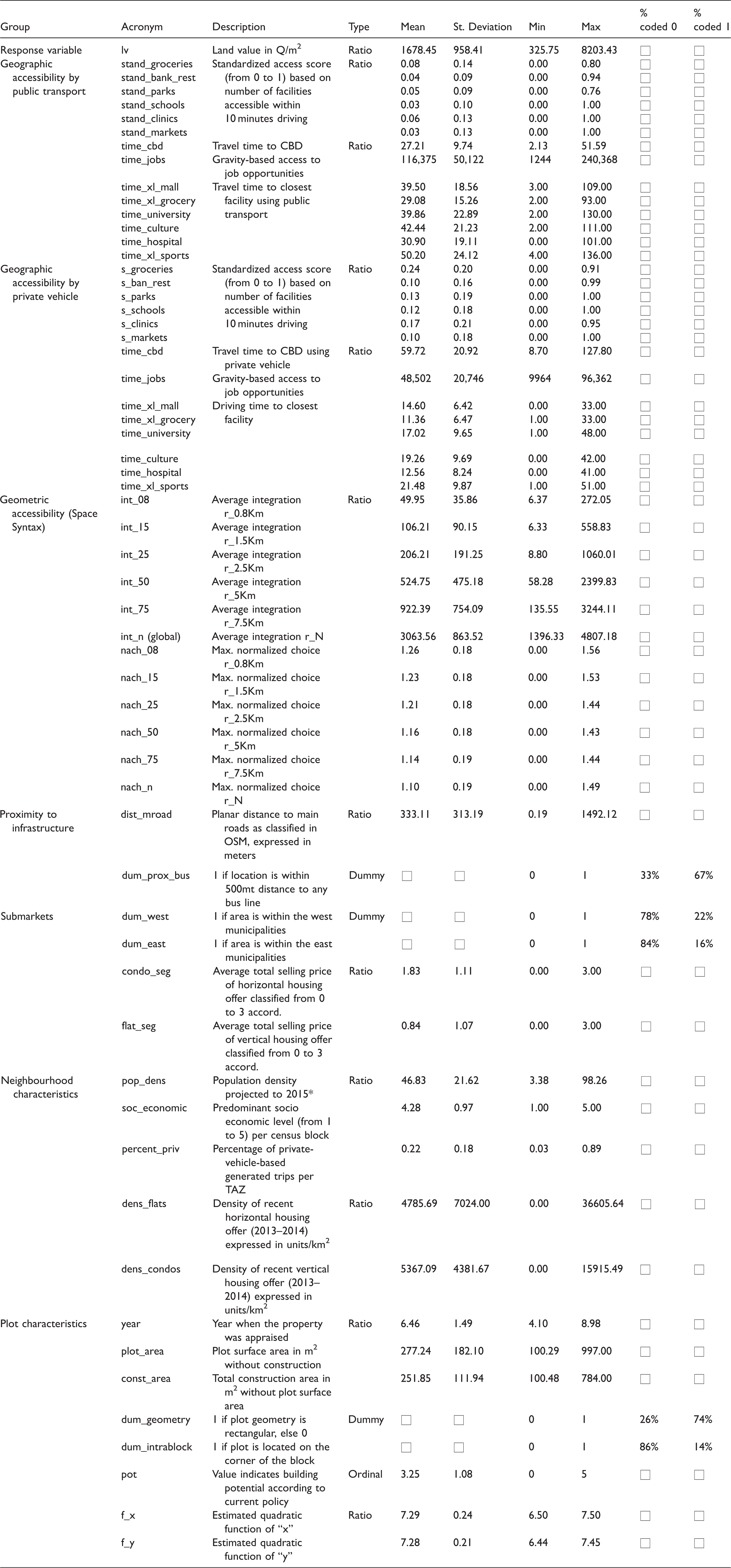
Grey highlighted cell indicates measurements that were transformed into natural logarithms (nl).

The CBD, jobs location, large-scale malls, large-scale groceries, universities, culture, hospitals and large-scale sport facilities are destinations for which people are more willing to overcome impedance, and influence location quality at a city scale. Access was measured as shortest travel-times, except for jobs access (Morales et al., 2016). This was mapped as potential access using the Hansen (1959) formulation. Decay parameters ( α , β ) were estimated using an origin-destination (OD) matrix containing trip volumes of traffic analysis zones (TAZ) per transport mode during morning peak-hours from year 2005. Travel-times were estimated for each OD pair. Then, trip volumes were ranked by travel-time and a decay function was fitted allowing to identify the optimum parameters for each transport mode. Values of trips attraction were calculated at the hexagon level. These were used as proxy values to indicate accessible jobs at each origin (hexagon centroids).

Geometric access includes SSx metrics, integration and choice, at various spatial scales (radii). High geometric access at lower radii (e.g. r_0.8 Km) benefit areas associated with pedestrian flows and important streets at a neighbourhood level. Access at higher or global (r_N) radii analyses benefit areas associated with important economic activity and reveal a roads hierarchy at a city-wide scale. Proximity to mobility infrastructure includes distance to main roads and whether or not a location is within a threshold distance of access points to a bus line.

Following Bourassa et al. (2007), we used submarket variables to address auto-correlated errors. Auto-correlated errors indicate the presence of a spatial structure due to nearby observations sharing similar locational and unmeasured externalities (Basu and Thibodeau, 1998; Lesage and Pace, 2009). Submarket classifications were mapped based on location (east or west periphery) and using expert knowledge from the AO. Submarket predictors classify the urban areas in reference to the selling-price segmentation of available new residential projects. Thus, indicating the non-existence of projects in an area (0), and the incremental selling-price coded from 1 to 3.

Neighbourhood characteristics include the following information: population density projected to 2015 (World_Pop, 2014); classification of socio economic groups per census track (Urbanistica, 2009); percentage of private mobility users per TAZ (percent_priv); and density of new residential projects. The “percent_priv” was estimated as the proportion of trips generated by private vehicles, from the total of trips generated per TAZ. Densities of new residential projects (dens_flats, dens_condos) were assumed to be able to capture popularity and demand for residential location. Geo-referenced locations of projects dating 2013 and 2014, provided by the AO, were processed using a point-density analysis at a 2 km radius (average neighbourhood size).

The year variable aimed to capture any temporal trend that was independent to monetary inflation. The plot surface area aimed to capture the relation where appraised value per m² decreases with increasing surface area (Lin and Evans, 2000). Construction area was a proxy variable included to isolate the land-value increase due to residence structural characteristics. We included dummy variables indicating whether the plot had a regular geometry or not, and the property intra-block location. These are locally used as appraisal “adjustment factors” (Dicabi, 2005). The POT variable, ranging from 1 to 5, attempted to capture the relation between the land-value with potential for future development into non-residential uses and/or larger constructions following current Territorial Ordinance Plan (DPU, 2009). Although it only applies for properties within Guatemala municipal boundaries, we classified the remaining plots using the same guiding principles.

Observation co-ordinates were used as predictors, also following Bourassa et al. (2007). Left side of Figure 2 shows initial scatterplots of each “x” and “y” co-ordinate at the upper and bottom areas correspondingly. Standardized co-ordinate values on the horizontal axis are plotted against land-values on the vertical axis. By fitting a quadratic function, the concave trends on both co-ordinates (x and y) reflect that the highest land-values are in the city core (matching CBD location) and these decrease as the co-ordinates move towards east or west (x co-ordinate), and south or north (y co-ordinate). Such trends were expected to be captured by the accessibility variables. Yet, we kept the co-ordinates as predictors to either capture any remaining trends or to reduce auto-correlated errors. Using the quadratic functions, we estimated new values to use as predictors (f_x and f_y) to remove the non-linearity. On the right side of the figure are the corresponding scatterplots.

Figure 2.

Scatterplots of x and y co-ordinates against the nl_land-values (left side); and scatterplots of estimated f_x and f_y plotted against nl_land-values (right side).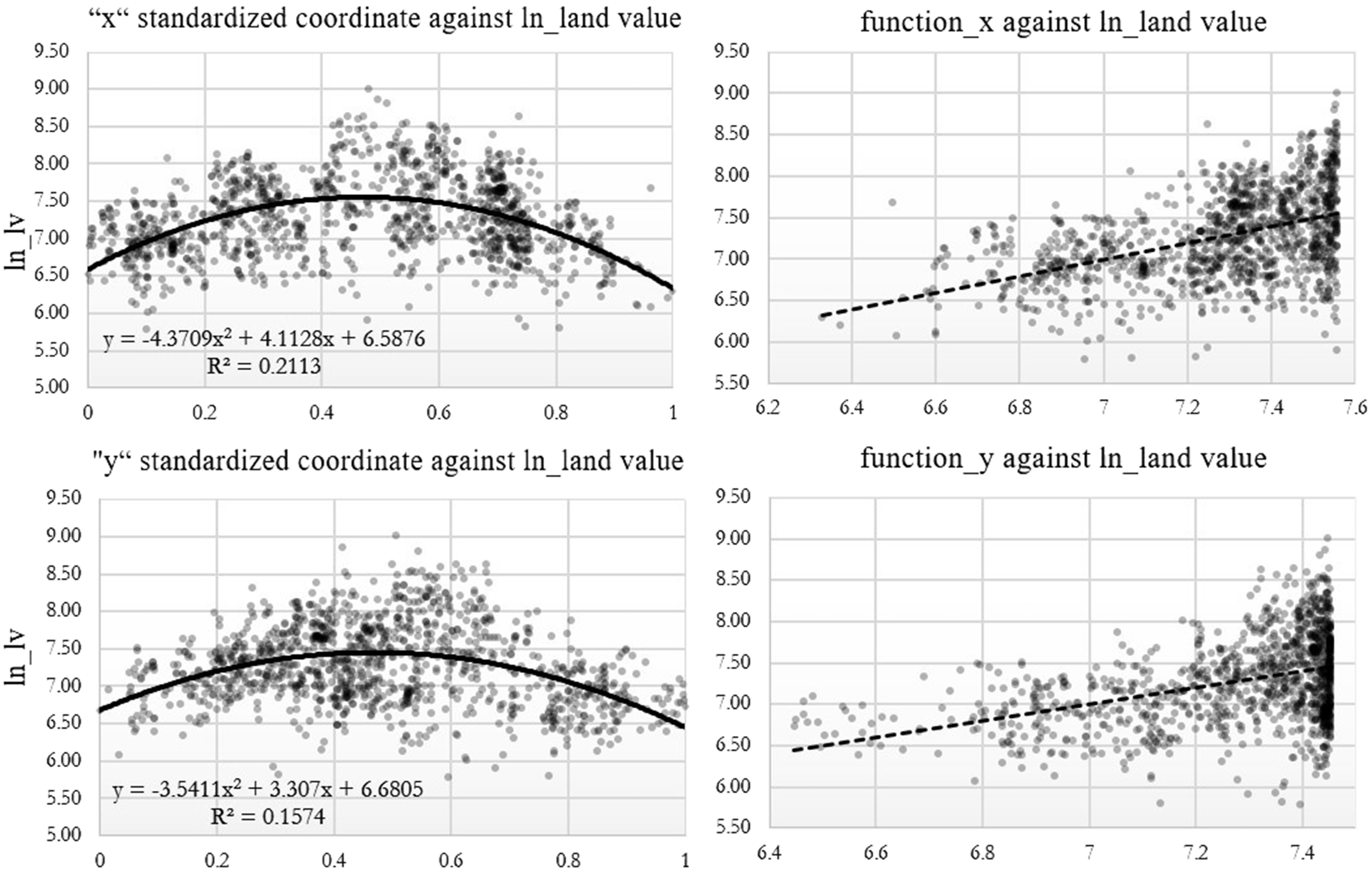

Methods

We used multivariate regression as a commonly accepted method in this research area, particularly in hedonic pricing studies. The regression model included the following access metrics: (1) geographic access indexes were computed based on travel-times per transport mode to various land uses; (2) geometric access incorporated SSx network metrics at various spatial scales; (3) we proposed a geometric via geographic-access metric formulated as the potential access to network integration (as measured in SSx). Additionally, other relevant variables were also included, such as submarket information, neighbourhood and property-level information. Following an initial correlation exploration, the model was first fully specified. Then, a variable selection process was implemented to assess the relevance of the information added by each variable and deduce the most parsimonious model. Finally, the model was assessed using performance statistics contrasted with alternative model versions representing common approaches in land-value modelling literature.

Geographic access indexes per facility were estimated using equation (1). Computations were done at the tessellation level for the entire city area. Access measurements per transport mode were all standardized to ranges from 0 (poor access) to 1 (high access). Then, combined_access to facilities at location i is given by the standardized access value by private vehicle times percent_priv , plus the equivalent formulation for access by public transport. Unlike Adair et al. (2000), our index was adjusted to the variation of the transport-mode predominance across the city. This variation is given by the percent_priv variable (see previous section), and represents the changing proportions of modal split aggregated to the hexagonal level. We assumed that areas where residents predominantly use public transport, public transport based access was locally more important compared to private-based access and vice-versa.

combined_{access}_{i} = (A_{priv}_{i} * perc_{priv}_{i}) + (A_{pub}_{i} * (100 - perc_{priv}_{i}))

(1)

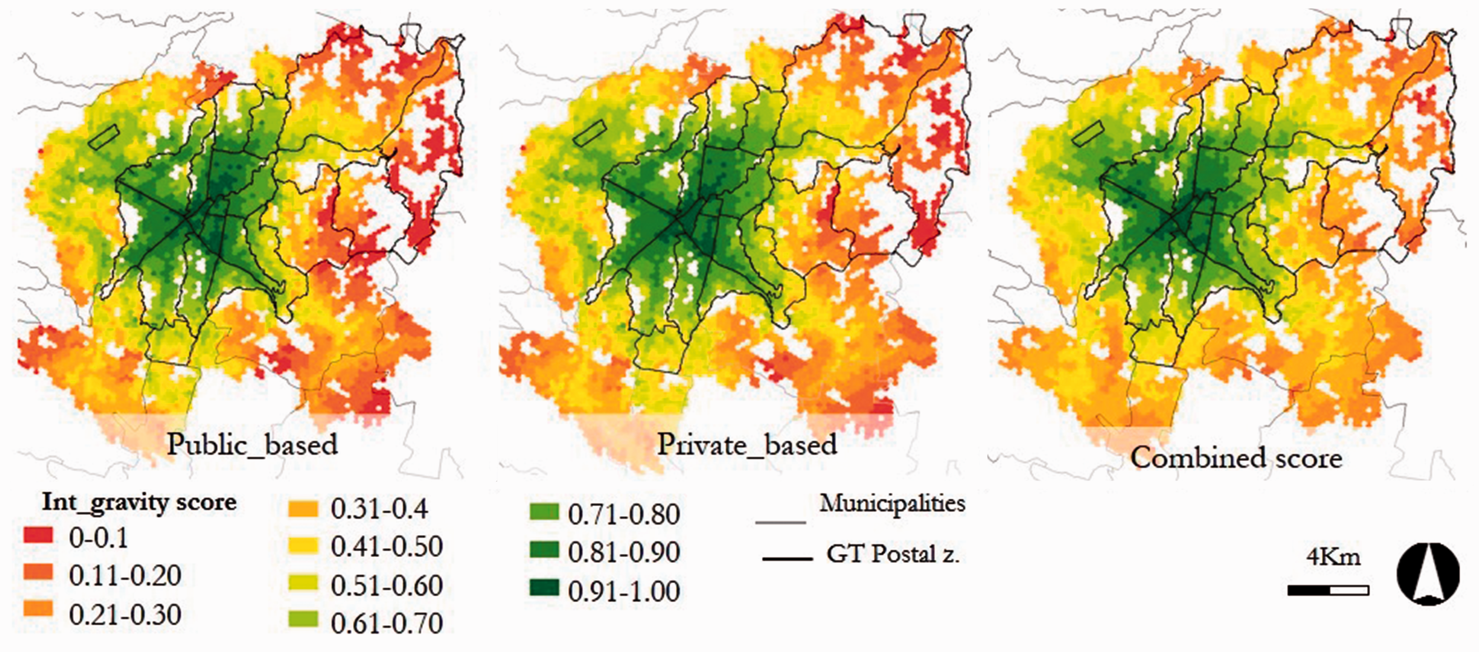
Geometric via geographic access was estimated as “ integration_gravity ” per hexagon i. We used equation (2), which is a potential access formulation (Hansen, 1959) where the attraction size is given by the average global integration (r_N) at any reachable hexagon, hex j, where n is equal to the number of segments in the system, and D_θ is the angular depth between a x segment and any other segment in the network, i (Hillier et al., 2012). We used global integration as it had the highest positive correlation with land-values. Decay parameters, α and β, exponentially penalize attraction size based on travel-time (t) between origin (hex i) and reachable destinations (hex j). The parameters applied in this computation were the same as used in Morales et al. (2016) to estimate job access: α = 1.2 for private and 1.3 for public transport; and β = 0.052 and 0.02 correspondingly. Although, this leads to potentially high collinearity with job access, it was still expected that integration_gravity would add additional information at a higher level of resolution. Figure 3 shows the results of implementing this metric.

integration_gravityhex i = \sum \frac{\overset{\sum}{(} (\frac{n - 1}{\sum_{i = 1}^{n} D_{θ} (x, i)}) hex j}{Nseg at hex j}) α exp (- β * t_{hex i - hex j})

(2)

Figure 3.

Geometric via geographic-accessibility from low (red) to high (green).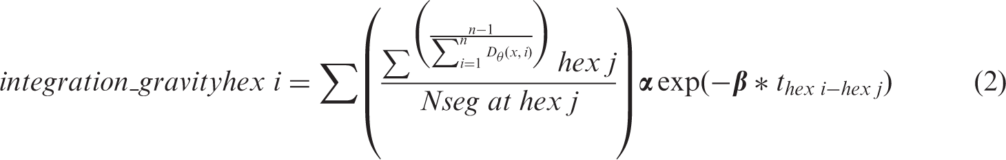

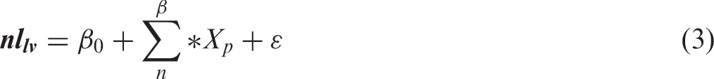
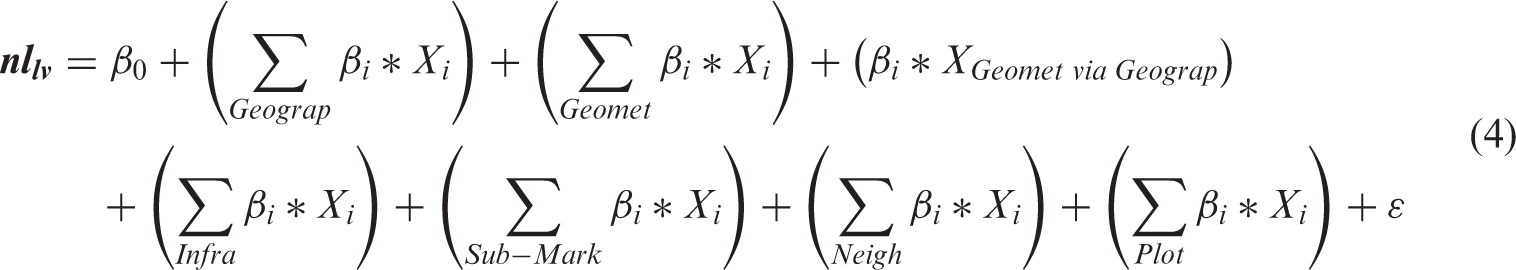
The regression model assumes that land-values can be decomposed into numerical contributions from the locational predictor attributes (Liu et al., 2010). A generalized specification follows equation (3). Where the land-value (nl_lv) of a property is estimated as a function of a constant intercept $β_{0}$ , plus the summation of the products between estimated coefficients (βi) with the measured attributes X, plus a random error ɛ.

{nl}_{lv} = β_{0} + \sum_{n}^{β} * X_{p} + ɛ

(3)

Our model takes the form of equation (4). Where the land-value predictors are grouped into geographic access, geometric access, geometric via geographic access, infrastructure proximity, submarket, neighbourhood and plot-level characteristics. The model was fitted via ordinary least squares in R software (Team, 2016) using 879 randomly selected observations (75%) to train the model, and the remaining observations for cross validation.

\begin{matrix} {nl}_{lv} = β_{0} + (\sum_{Geograp} β_{i} * X_{i}) + (\sum_{Geomet} β_{i} * X_{i}) + (β_{i} * X_{Geomet via Geograp}) \\ + (\sum_{Infra} β_{i} * X_{i}) + (\sum_{Sub - Mark} β_{i} * X_{i}) + (\sum_{Neigh} β_{i} * X_{i}) + (\sum_{Plot} β_{i} * X_{i}) + ɛ \end{matrix}

(4)

It was expected that not every predictor would add meaningful information to the model and that access variables would introduce some multicollinearity, which makes almost impossible to discriminate predictors based on their coefficients and significance. Therefore, we applied an automated bi-directional stepwise regression using the MASS package (Ripley et al., 2002), where variables are retained or discarded based on their contribution to the Akaike Information Criterion (AIC) statistic (Bozdogan, 1987). For the final reduced model we used the Breusch–Pagan test and White’s correction to correspondingly detect heteroskedasticity and adjust the coefficients, and the Variation Inflation Factor (VIF) to detect multicollinearity (Fox and Weisberg, 2011).

The estimated coefficients represent the impact of each variable on the land-value. However, those are not comparable among each other as they are scale-dependant. First, not all the predictors are expressed in the same units (e.g. logarithmic scales versus standardized access-scores). Second, the predictor values come from a systematic mapping for the whole city area. So, the value ranges differ even for predictors expressed in the same units (Table 1). Therefore, standardized beta-coefficients (Fletcher, 2015) are also reported.

We used the following performance statistics to assess the models: adjusted R², AIC, semivariogram modelling to assess the presence of auto-correlated errors (Gräler et al., 2016), the root mean squared error over prediction (RMSEP) of test-data and the normalized RMSEP to compare the proportional difference of error variance among models. The RMSEP used the difference between the maximum and minimum observed values of the test-data (2.82).

Semivariogram models assume that the similarity between any pair of residuals is inversely proportional to the lag (distance) between them. Dissimilarity is estimated as gamma values. Three parameters can be read from the semivariogram: (1) the nugget is the value of gamma at lag = 0 and associated to statistical noise; (2) the partial sill is the difference between the nugget and the value of gamma when auto-correlation becomes negligible; (3) the range indicates the distance between observations where auto-correlation becomes negligible and the partial sill is reached. The variograms fitted here are exponential and assume isotropy, meaning that the spatial dependence at a given lag is constant throughout the area and that the resulting range is effective up to three times its distance.

The model was assessed in comparison to six alternative models, which were formulated as variations of equation (4) and estimated using the same approach. First and second are model variations where corresponding access predictors only address one of the transport modes. The third model is as the original, but excludes all of the geometric-access predictors. The fourth considers exclusively a mono-centric assumption and excludes potential jobs access. In turn, the fifth model replaces CBD access with potential job access, relaxing the mono-centric assumption. The sixth model is a variation that excludes all of the submarket predictors and the observations co-ordinates.

Results and discussion

Accessibility and land-values

Figure 4 shows pairwise correlations between the access metrics relying on transport modes (geographic access and geometric via geographic access) with the land-values. Correlations of the private and public transport-based access metrics were included for reference purposes. A label indicates in which definition each metric (travel time, cumulative opportunity or potential access) was originally measured.

Figure 4.

Pearson’s correlations between accessibility metrics and nl_land-value.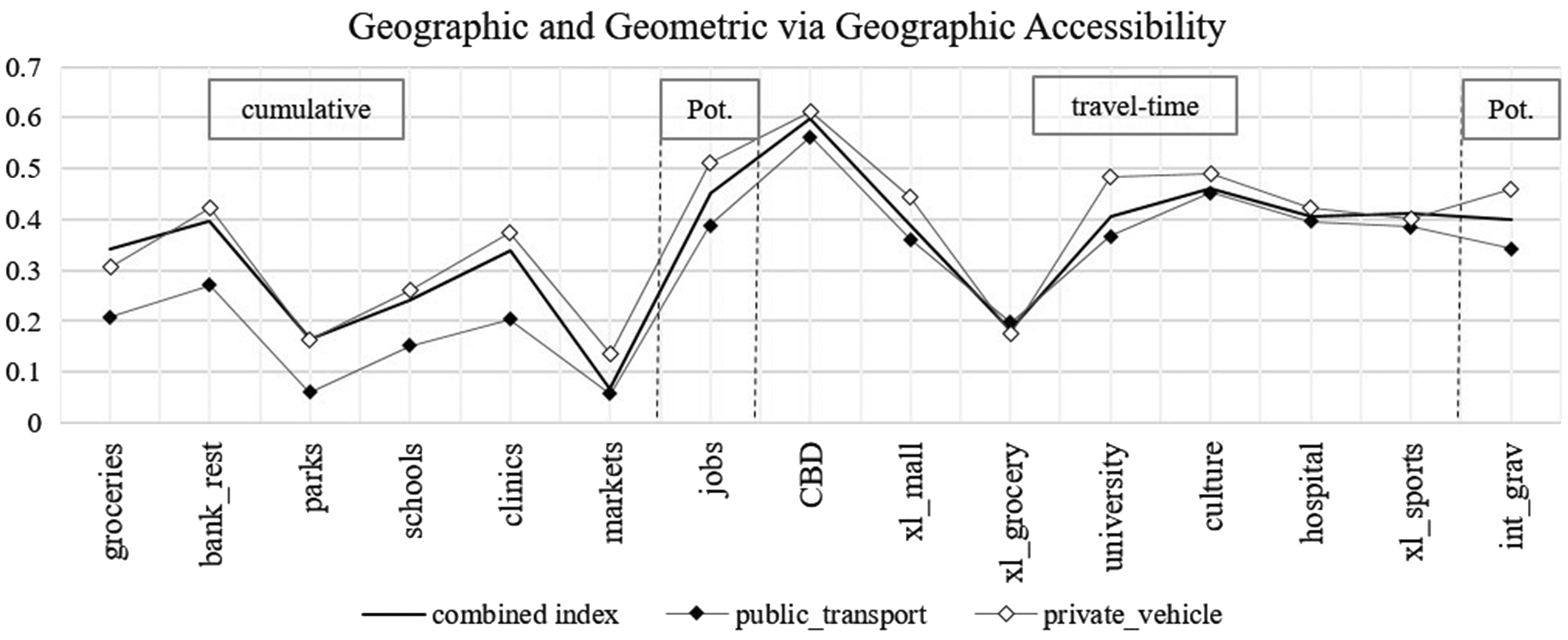

The strengths of the correlations for each variable are similar for both transport modes except for the first five land uses. Private mobility strongly increase access opportunities to concentrations of such land uses. This is reflected in higher pairwise correlations with higher land-values in contrast with access by public mobility. This comparison seems applicable to all the variables considered. However, cumulative-opportunity metrics, aiming to analyse quality location at a neighbourhood scale, made the mobility disparity more evident.

Correlation strengths of the combined indices fall between the correlation strengths by transport mode. This was expected as the indices incorporate and reflect the difference on the strength of the pairwise correlations by transport mode, previously discussed. However, the combined indices are sensitive to spatial variations of the access benefits derived from simultaneous availability of transport modes as well as to the residents’ predominant preference for those. This was expected to contribute with additional information to the model, compared to only addressing one transport mode.

Importance of a monocentric land-value structure is preliminarily detected as the strongest correlation is observed with CBD access (∼0.6). Access to jobs, geometric via geographic access (integration_gravity), universities, cultural institutions and large-scale malls reach correlations up to ∼0.5. Then, access to banks and restaurants, clinics, hospitals and large-scale sports infrastructure reach correlations up to 0.4.

Figure 5 shows correlations of the geometric access metrics that were computed via SSx. Geometric access metrics, estimated via SSx, all show positive correlations. Those increase when increasing the radii of analysis (0.8 km-Global), from 0.09 to 0.16 for the choice values and from 0.07 to 0.4 for the integration values. This means that, at first glance, geometric-access is a quality-location that tends to be more important when indicating relative location to the city as a whole and lesser at the neighbourhood scale. Also, compact grids with small blocks are less favoured than longer blocks.

Figure 5.

Pearson’s correlations between geometric accessibility and nl_land-value.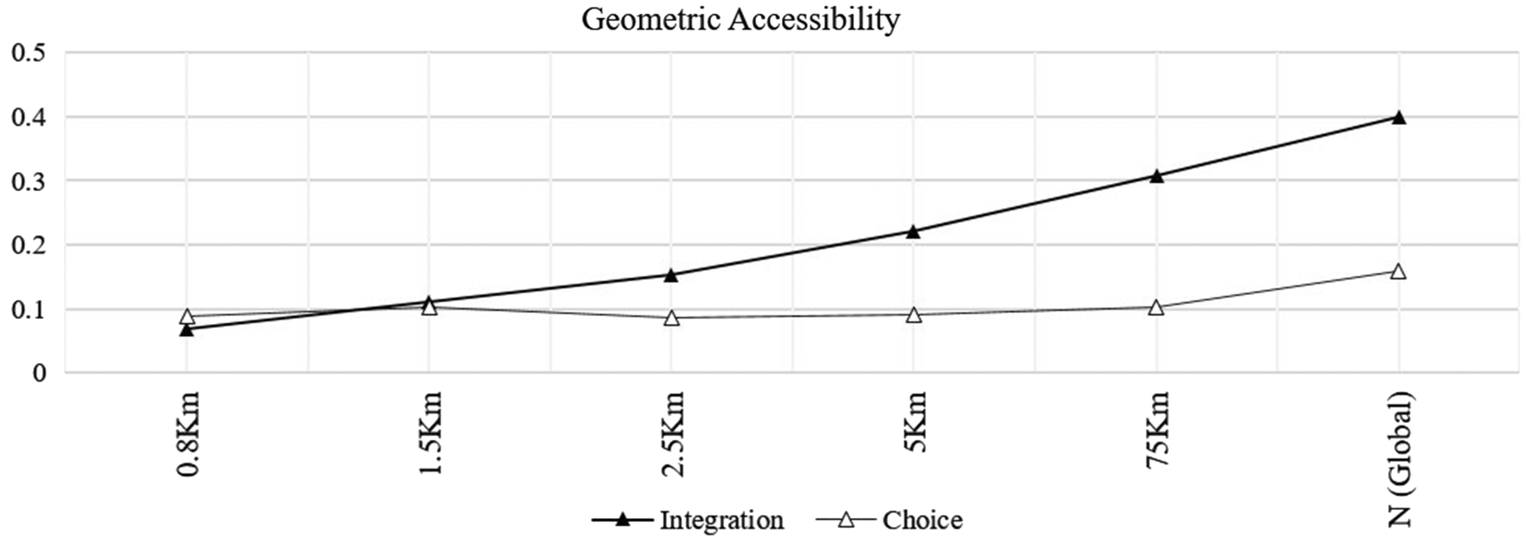

Table 2 shows model results after the variable selection process. Only relevant variables were kept in the model based their information contribution, reflected through the AIC statistic. Variables expressed in logarithmic form are interpreted as the percentage change in land-values per 1% change in the predictor value. This is also applicable to coefficients of indices ranging from 0 to 1 (i.e. geographic and geometric via geographic access). Other coefficients are interpreted as the percentage change in land-values given 1 unit change in the predictor.

Table 2.

Regression coefficients and normalized coefficients. Grey colour bars on the normalized coefficients indicate relative importance.

Predictors		Coeff.	Std. error	t	Significance		VIF	n_coeff.
	Intercept	−0.32	1.09	−0.28	0.77
Geographic accessibility	access_groceries	□	□	□	□		□	□
	access_ban_res	0.80	0.22	3.62	0.00	***	3.6	0.15
	access_parks	□	□	□	□		□	□
	access_schools	0.42	0.17	2.38	0.02	*	2.8	0.09
	access_clinics	□	□	□	□		□	□
	access_markets	□	□	□	□		□	□
	access_cbd	2.53	0.45	5.55	0.00	***	19.0	0.47
	access_jobs	−1.26	0.29	−4.42	0.00	***	48.7	−0.50
	access_xl_mall	1.16	0.24	4.75	0.00	***	7.2	0.23
	access_ xl_grocerie	−1.17	0.20	−5.85	0.00	***	4.0	−0.20
	access_university	1.21	0.22	5.50	0.00	***	7.7	0.26
	access_culture	−1.87	0.38	−4.87	0.00	***	21.0	−0.40
	access_hospital	1.21	0.24	5.01	0.00	***	7.4	0.24
	access_xl_sport	□	□	□	□		□	□
Geometric accessibility	nl_int_08	−0.09	0.03	−2.80	0.01	**	4.1	−0.10
	nl_int_15	□	□	□	□		□	□
	nl_int_25	−0.12	0.03	−3.77	0.00	***	7.2	−0.18
	nl_int_50	□	□	□	□		□	□
	nl_int_75	□	□	□	□		□	□
	nl_int_n (global)	0.28	0.11	2.51	0.01	*	11.9	0.16
	nl_nach_08	□	□	□	□		□	□
	nl_nach_15	0.38	0.13	3.00	0.00	**	1.5	0.07
	nl_nach_25	□	□	□	□		□	□
	nl_nach_50	□	□	□	□		□	□
	nl_nach_75	□	□	□	□		□	□
	nl_nach_n	□	□	□	□		□	□
Geomet. via Geog.	access_int_grav	0.62	0.30	2.07	0.04	*	47.1	0.26
Proximity to infrastructure	dist_mroad	□	□	□	□			□
Proximity to infrastructure	dum_prox_bus	−0.11	0.02	−4.22	0.00	***	2.0	− 0.10
Submarket variables	dum_east	0.25	0.08	3.23	0.00	**	9.2	0.19
	dum_west	−0.10	0.04	−2.67	0.01	**	3.3	−0.07
	condo_seg	0.07	0.02	3.95	0.00	***	4.2	0.16
	flat_seg	0.09	0.02	5.01	0.00	***	4.1	0.20
Neighbourhood characteristics	nl_pop_dens	0.12	0.03	3.78	0.00	***	6.4	0.16
	soc_economic	0.04	0.01	3.49	0.00	***	1.3	0.07
	perc_private	0.33	0.09	3.74	0.00	***	2.4	0.11
	nl_dens_flats	0.01	0.00	3.59	0.00	***	2.3	0.09
	nl_dens_condos	0.01	0.01	2.09	0.04	*	2.2	0.06
Plot characteristics	year	0.09	0.01	17.46	0.00	***	1.1	0.34
	nl_plot_ar	−0.17	0.03	−6.15	0.00	***	2.1	−0.19
	nl_const_ar	0.14	0.04	3.68	0.00	***	2.0	0.11
	dum_geometry	□	□	□	□		□	□
	dum_intrablock	□	□	□	□		□	□
	pot	□	□	□	□		□	□
	f_x	0.29	0.07	3.82	0.00	***	4.4	0.13
	f_y	□	□	□	□		□	□

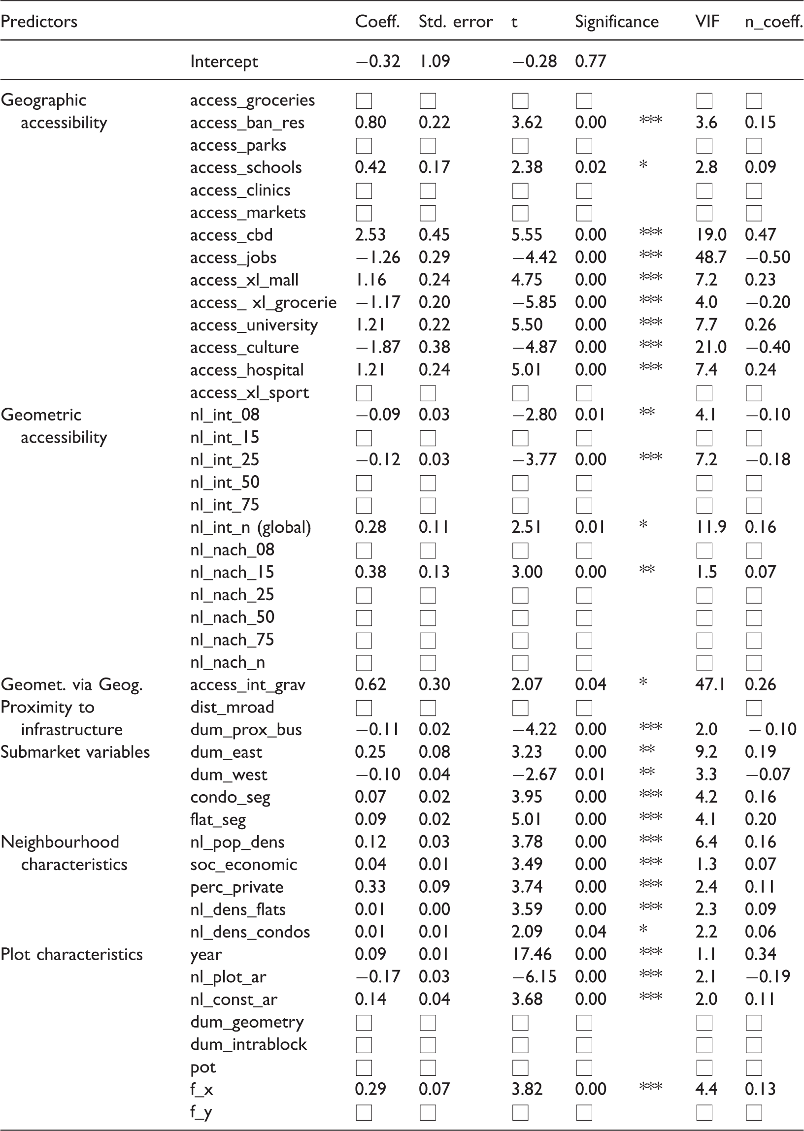
VIF: Variation Inflation Factor.

Significance: ***0.001, **0.01, *0.05.

From the cumulative access metrics, only access to banks and restaurants and schools were retained. Both have a positive impact of 0.80% and 0.42% per 1% increase of access to those facilities. A 1% increment in CBD access has a positive impact of 2.53% on the value of land. Meaning that land-values at the CBD are ∼253% more expensive than those at periphery. Job access has an unexpected negative sign. Values decline 1.26% per 1% increase in the access index. We tested the sign reversal by manually removing, one by one, the following predictors that showed multicollinearity and correlation with job access: integration_gravity, global integration, CBD and culture access. Nevertheless, we found the sign remained negative. We hypothesise that in our case study when adding job access to the model simultaneously with other predictors, the index might be actually capturing the negative effects of urban centrality (e.g. pollution and congestion). Particularly when considering that this metric uses the number of trips attracted to an area as a proxy to availability of jobs.

Land-value increases by 1.16% with a 1% increase in access to large-scale malls. In turn, a 1% increase in access to large-scale grocery shops means a decline of 1.17%. The comparison between these two coefficients could be revealing that the attractiveness of agglomerated commerce and recreational activities is the one that overweighs the potential negative impacts (noise and congestion) that the vicinity of either facility poses. Furthermore, a 1% increase in the access score of the following externalities implies an increase of land-values: universities (1.21%) and hospitals (1.21%). Unexpectedly, access to cultural facilities has a negative effect of a 1.87% decrease in land-values. In Guatemala City, cultural facilities are mostly located in the core and historic areas of the city. Negative externalities, such as pollution, congestion, street robbery, and informal commerce are common in these areas, which could explain the positive association with the land-values in the pairwise correlation, but a negative sign when placed jointly with other predictors.

As in Chiaradia et al. (2009), SSx integration has contrasting effects according to the analysed spatial scale. An increase of 1% in integration at lower radii (0.8 km and 2.5 km) implies a decline of land-values of 0.09% and 0.12% correspondingly. In Guatemala City most of the areas highlighted at low radii integration correspond to deteriorated single family neighbourhoods. These are areas with compact gridiron street patterns built during the first planned expansions. Middle-low and low-income groups predominantly reside in these areas, vulnerable to pollution and street robbery. In turn, the effect of integration is positive at a city-wide scale (global). Land-values increase by 0.28% per 1% increase of global integration. SSx choice at 1.5 km has a positive impact of 0.38%. Neither distance to main roads nor normalized choice at higher radii were selected. From the results we interpret that residential land-values benefit only when located nearby streets that are important at a neighbourhood scale, even tough, such streets are commonly part of or are connected to city-structuring roads outlined by choice analyses at higher radii.

Geometric via geographic access has a positive influence of 0.62% per 1% increase in the access index, implying that quality locations benefit from geometric access not only at location, but also as a reachable resource. This metric might be capturing access to vital urban areas, or with potential for doing so, containing economic activities not addressed explicitly by the other predictors.

The strongest multicollinearity (VIF ∼50) was observed with jobs and geometric via geographic access, meaning, as expected, there is a strong correlation between them and implying that their interpretation should not be considered without caution. However, we are able to claim that each predictor still adds complementary information to the model following their impact on the AIC statistic. This is further discussed in the model assessment.

Observations within a 300 m distance of the bus lines network showed a decline of 0.11%. This was expected as previous access predictors address the true benefit of public transport, while the mere physical proximity to the network itself might be associated with negative externalities such as noise and pollution.

We observe a difference between the sub-market variables indicating east and west peripheral municipalities. Assuming that the rest of the variables are held constant, residential land on the eastern periphery is more expensive by 0.25% compared to the rest of the observations, whereas land is 0.10% cheaper in the western peripheral areas. For the average plot, this means a difference of +Q445/m² ($60) and –Q115/m² ($15) respectively. Density of new condominiums predominates in both peripheral areas, particularly at the west. However, selling price segmentation clearly points out a more expensive market at the peripheral east side. Selling-price segmentation of residential projects (horizontal and vertical) have both a positive impact of 0.07% and 0.09% on the land-value.

Neighbourhood characteristics all have a positive contribution. An increase of 1% in the population density represents higher land-values by 0.12%. The predominance of different socio-economic groups, incremental from 1 (low incomes) to 5 (high incomes), is associated with a land-value increase of 0.43%. This is equivalent to a difference of Q345/m² (∼$45) for an average plot located either in an area classified as 1 or 5. An increase of 1% in the proportion of private vehicle users in an area is associated with a land-value increase of 0.33%. Furthermore, an increase of 1% in density of new vertical and horizontal residential projects has a positive influence of 0.01%. This is equivalent to a difference of ∼5–7 new residential projects within a radius of 2 km.

The coefficient of the year predictor reveals that in these data there is an increase in the land-values of 0.09% every year. Such value increase over time is additional to money inflation. This variable could be reflecting the influence of dynamics that were not captured by any other predictor. For example, urban transformations along time (e.g. city expansion, redevelopment) and overall macroeconomic growth. The average annual growth of the gross domestic product (GDP) per capita was 0.93% between 2008 and 2014 (Bank, 2017). Furthermore nl_land-value per m² is appraised 0.17% lower per 1% increase in the plot surface area. In turn, a 1% increase in built-up areas has a positive impact of 0.14%. Lastly, the co-ordinate function f_x reflects an increase of 0.29% per one unit increase, meaning that there is a value increase trend along the east-west direction additional to the access benefits and any other location characteristic addressed by the predictors included.

Finally, the normalized coefficients can be interpreted as changes in standard deviations of the land-values per one standard deviation change in the predictor variable. These coefficients are comparable. Access to CBD was the most important variable that positively influenced the residential land-values in Guatemala City, thus confirming a mono-centric land-value structure. It is followed by the year predictor, outlining the relevance of land-value gains over the years. Interestingly, geometric via geographic accessibility becomes the third most important predictor that capitalizes residential land, then followed by access to universities, malls and hospitals.

Model performance and diagnostics

Table 3 shows a summary of the performance statistics of our original model, contrasted with the alternative models. Those represent existing land-value modelling approaches. The upper part of the table indicates the predictors that were excluded from the initial model formulations, and the predictors kept in each model after the variable selection procedure.

Table 3.

Model performance in contrast with alternative models.

Predictors		Original	1. Public	2. Private	3. Geographic	4. CBD	5. Jobs	6. Without Sub-Markets
Geographic accessibility	access_groceries				✓
	access_ban_res	✓	✓			✓	✓	✓
	access_parks
	access_schools	✓	✓	✓			✓
	access_clinics				✓	✓		✓
	access_markets			✓			✓
	access_cbd	✓	✓	✓	✓	✓	□	✓
	access_jobs	✓	✓		✓	□	✓
	access_xl_mall	✓	✓	✓	✓	✓	✓	✓
	access_ xl_grocerie	✓	✓	✓	✓	✓	✓	✓
	access_university	✓	✓	✓	✓	✓	✓	✓
	access_culture	✓	✓	✓	✓	✓	✓	✓
	access_hospital	✓	✓	✓	✓	✓	✓	✓
	access_xl_sport
Geometric accessibility	nl_int_08	✓	✓	✓	□	✓	✓	✓
	nl_int_15				□
	nl_int_25	✓	✓	✓	□	✓	✓
	nl_int_50				□			✓
	nl_int_75				□
	nl_int_n (global)	✓	✓	✓	□	✓	✓	✓
	nl_nach_08				□
	nl_nach_15	✓	✓	✓	□	✓	✓	✓
	nl_nach_25				□
	nl_nach_50				□			✓
	nl_nach_75				□
	nl_nach_n		✓		□		✓
Geomet. via Geog.	access_int_grav	✓	✓	✓	□		✓	✓
Proximity to infrastructure	dist_mroad
Proximity to infrastructure	dum_prox_bus	✓	✓	✓	✓	✓	✓	✓
Submarket variables	dum_east	✓	✓	✓	✓	✓	✓	□
	dum_west	✓	✓	✓	✓	✓	✓	□
	condo_seg	✓	✓	✓	✓	✓	✓	□
	flat_seg	✓	✓	✓	✓	✓	✓	□
Neighbourhood characteristics	nl_pop_dens	✓	✓	✓	✓	✓	✓
	soc_economic	✓	✓	✓	✓	✓	✓	✓
	percent_private	✓	✓	✓	✓	✓	✓	✓
	nl_dens_flats	✓	✓	✓	✓	✓	✓	✓
	nl_dens_condos	✓		✓	✓	✓		✓
Plot characteristics	year	✓	✓	✓	✓	✓	✓	✓
	nl_plot_ar	✓	✓	✓	✓	✓	✓	✓
	nl_const_ar	✓	✓	✓	✓	✓	✓	✓
	dum_geometry		✓			✓	✓	✓
	dum_intrablock
	pot							✓
	f_x	✓	✓	✓	✓	✓	✓	□
	f_y		✓	✓			✓	□
Goodness of fit	Adjusted R²	0.728	0.704	0.718	0.711	0.723	0.720	0.687
Goodness of fit	AIC	167	243	199	213	180	192	274
Auto correlated errors	Nugget	0.0055	0.0053	0.0059	0.0059	0.0053	0.0049	0.0060
	Partial Sill	0.0611	0.0671	0.0627	0.0675	0.0625	0.0624	0.0678
	Effective range (m)	741	763	771	938	734	703	942
Cross validation	RMSEP	0.3177	0.3184	0.3183	0.3211	0.3203	0.3136	0.3373
Cross validation	N_RMSEP	0.1127	0.1129	0.1129	0.1139	0.1136	0.1112	0.1196
□ predictor excluded ✓ predictor selected

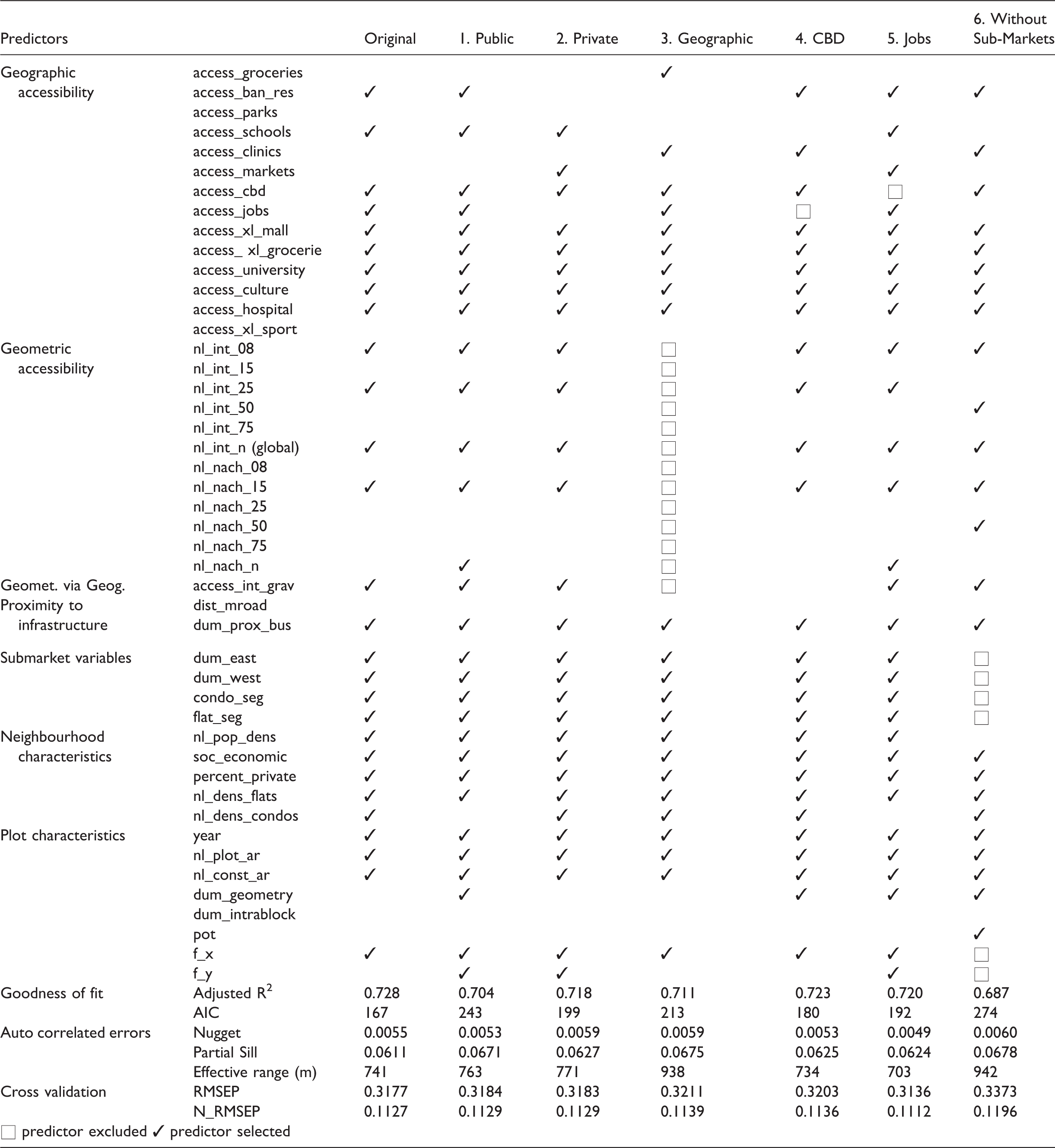
The original model was found to have the highest performance of all the models. It has the highest goodness of fit over the train data explaining up to 72.8% of the land-values variability. It has the lowest AIC value (167), meaning it is the most parsimonious model and closer to reflect the process that generates the land-value observations. Comparison of the AICs reflects an improvement of 31% and 16% over a model based only on public (1st) and private (2nd) mobility correspondingly. Furthermore, it improves by 22% over a model that excludes geometric access information (3rd). We do not observe major differences (up to 4%) in the adjusted R² across the models. However, judging by the AIC comparisons, there is an important improvement in the land-value modelling approach when addressing more than one transport mode.

By comparing the original model against the 4th and 5th alternatives, we determined that together both CBD and “jobs” access contribute to a better model. It is clear that CBD access is a dominant predictor when considering its estimated coefficient (Table 2) and observing its effect on the AIC statistic when excluded in the 5th model, while some caution should be taken when interpreting what is being revealed by “jobs access” given its sign reversal and its multicollinearity with the CBD and the geometric via geographic-access itself.

Furthermore, it seems that addressing geometric accessibility does not only improve the goodness of fit, but also reduces the spatial dependence of the regression residuals by almost 200 m, meaning that less variability in the land-value observations is left unexplained and indicating that geometric access predictors add spatialized information at a localized scale. Such information is comparable to the information that is contributed to the model by the submarket predictors and the observation co-ordinates. This is also deduced from observing the AIC statistic of the 6th model, and the increase of geometric access predictors being kept in this model.

The cross-validation with the test data shows that variations of prediction accuracy among models are modest. The original model shows the lower RMSEP (0.3150), which is equivalent to 1.37 units in local currency. The N_RMSEP shows that the standard deviation of the prediction errors for all the models remains relatively the same. These statistics were somehow unexpected. However, even at this minor scale, the highest differences are observed when excluding geometric-access and the submarket predictors.

Finally, Figure 6 shows the regression diagnostics. From left to right, we observe that the dispersion of the residuals follows an approximately constant variance. The QQ plot shows that prediction errors closely follow a normal distribution. The plot on the right shows that errors are mostly centred in 0, with a slight tendency to overestimate extremely low values and underestimate extremely high values. This indicates a slight non-linearity behaviour in the data. However, by visually judging this figure and considering the magnitude of the errors in the cross-validation, we determined that such behaviour has minor effects in the performance of the model.

Figure 6.

Diagnostics of model residuals.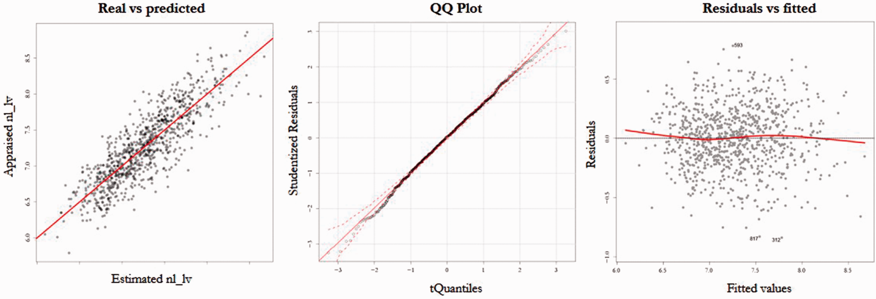

Conclusions

We implemented a comprehensive operationalization of accessibility indicators to develop a residential land-value model in Guatemala City. The model incorporated metrics of geographic, geometric and geometric via geographic access. Those were computed as indices that incorporate the variation of the access disparity due to current availability of transport modes and adjusted to the predominant use of each mode across the city.

Following our first hypothesis, land-value research would benefit from considering more comprehensive definitions of accessibility. Integrating the available transport modes into the model modestly improved the goodness of fit to the observed data (adjusted R²) and the prediction accuracy of non-observed data. Nevertheless, it yielded a model that better represents the true process generating the observations (AIC), compared to similar models addressing access by only one transport mode. Furthermore, geometric accessibility brings spatialized and localized information that contributes to a parsimonious model and better explains the variability of land-values. This was deduced from observing a reduction of the spatial dependence in the model residuals.

Following our second hypothesis, we conclude that geometric accessibility does capitalize land at location (to some extent) and as a reachable resource. Similar to the results of Chiaradia et al. (2009), integration (network closeness), analysed at a localized radius of 0.8–1.5 km, has a negative effect on residential land-values. In Guatemala City, local integration outlines areas with compact gridiron layouts in old neighbourhoods. In turn, relative closeness to anywhere in the city in areas with larger blocks seems to capitalize land-values. Only hierarchy of roads on the neighbourhood scale, as analysed by SSx choice (network betweenness), has a positive impact on residential land-values. Furthermore, we determined that the potential reachability of geometric access by available transport modes is positively associated with the value of land. We consider this metric as complementary, as it could reflect access to economically vital areas (or with the potential for such) not addressed explicitly in other access metrics.

From the model results, we found that land-values in Guatemala City differ up to 253% following CBD access, which was the strongest predictor. Thus, we conclude that there is a predominance of a mono-centric land-value structure, which strongly reflects centralized economic activities, as described by Ford (1996). Access to jobs was the most important negative externality. We assume that when other predictors better explain such opportunities, this metric reveals the negative effects of urban centrality (pollution and congestion), also considering that it is computed using trips attraction as a proxy of job opportunities.

The results have some limitations and open a few paths for further research. Geographic access metrics per transport mode might bring multicollinearity problems when using a multivariate regression method. In this research we addressed this situation by computing access indices that, unlike Adair et al. (2000), are weighted by the predominance or preference for each transport mode across the city. However, it is necessary to consider potential mobility shifts along time, to test improvements by using other approaches to estimate the indices, or to use other regression techniques to deal with multiple collinear predictors. Unlike Bourassa et al. (2007), the use of submarket variables and geographic co-ordinates did not fully remove spatial dependence, meaning that some unexplained localized information could be further addressed with the help of spatial econometrics or geostatistical approaches. The ability of the geometric via geographic accessibility variable to explain land-values should be investigated in different urban contexts. Different time-decay parameters could increase or reduce the information that is added to the land-value model.

Several Latin American cities show centralized economic activities reflected in mono-centric structures, similar to Guatemala City. Yet, Guatemala City also has its unique characteristics such as the urban form, topography, immediate proximity of the airport with the CBD, arrangement of main infrastructure and particular local values, meaning that the methodological approach presented in this research could be replicated to other Latin American cities and other areas, but not without adjusting it by using local knowledge.

Finally, some implications can be drawn for planning and land administration practice. More robust models for mass valuation purposes, with added transparency to the process, could be achieved by simultaneously addressing public and private accessibility from a geographic perspective. Furthermore, it could be relevant for transport planners to explicitly model the relations between accessibility by public transport infrastructure and the value of land. In developing countries, this could mean producing useful information to help the planning of transport projects in relation to the attractiveness and capitalization of land. Moreover, the approach could be an initial step towards foreseeing the potential impact of mobility-related projects on land-value. This is of great relevance to ground different financial mechanisms to enforce the economic viability and sustainability of projects such as land-value captures.

Footnotes

Acknowledgements

We would like to thank the collaboration by local experts from “Inspecciones Globales” in Guatemala City for their support on collecting real estate appraisals data, and granting access to their reports on the local real estate market.

Declaration of conflicting interests

The author(s) declared no potential conflicts of interest with respect to the research, authorship, and/or publication of this article.

Funding

The author(s) disclosed receipt of the following financial support for the research, authorship, and/or publication of this article: The work reported in this research was funded by NUFFIC through the NICHE Project.

Jose Morales holds a degree in Architecture (2009) from Istmo University in Guatemala. He worked during two years and a half at the Urban Planning Bureau of Guatemala City. In 2011 he started his master’s studies in ITC Faculty, University of Twente. In 2013 completed his MSc in Geoinformation Science and Earth Observation applied to Urban and Regional Planning. He develops his current research in the same university. His research interests are urban accessibility, residential land values, participatory planning, sustainable housing.

Dr Johannes Flacke holds a Diploma degree in Geography (1994) from Ruhr-University Bochum in Germany. He received his PhD in Geosciences at the Ruhr-University Bochum in 2002 with a dissertation on information systems promoting sustainable land use based on spatial indicators. Before joining ITC at the University of Twente as assistant professor Spatial Planning and Decision Support Systems in 2007 he worked as a post-doc researcher at the Department of Urban and Regional Planning, TU Dortmund University.

Prof. Dr. Jaap Zevenbergen has a Doctors degree (PhD) on Systems of Land Registration of Delft University of Technology (2002). In 1990 he graduated in Geodetic Engineering from the former Faculty of Geodesy, Delft University of Technology, and in 1992 in Dutch Law from the Faculty of Law, Leiden University. Between 1989 and 2003 he worked first as research assistant and later as assistant professor in the Faculty, later Department, of Geodesy, and between 2003 and 2010 as associate professor at the OTB Research Institute for Urban, Housing and Mobility Studies. In 2008 he was appointed professor in Land Administration Systems within the Department of Urban and Regional Planning and Geo-information Management (PGM) of the ITC, University of Twente.

References

Adair

Mcgreal

Smyth

et al. (2000) House prices and accessibility: The testing of relationships within the Belfast urban area. Housing Studies 15: 699–716.

Ahlfeldt GM (2007) If Alonso was right: Accessibility as determinant for attractiveness of urban location. Hamburg contemporary economic discussions.

Ahlfeldt

Wendland

(2011) Fifty years of urban accessibility: The impact of the urban railway network on the land gradient in Berlin 1890–1936. Regional Science and Urban Economics 41: 77–88.

Alonso

(1964) Location and Land Use: Towards a General Theory of Land Rent, Cambridge, MA: Harvard University Press.

Anantsuksomsri

Tontisirin

(2015) The impacts of mass transit improvements on residential land development values: Evidence from the Bangkok Metropolitan Region. Urban Policy and Research 33: 195–216.

Bafna

(2003) Space syntax: A brief introduction to its logic and analytical techniques. Environment and Behavior 35: 17–29.

Bank W (2017) GDP per captia growth in Guatemala [Online]. Available at: http://data.worldbank.org/indicator/NY.GDP.PCAP.KD.ZG?end=2015&locations=GT&start=2001&view=chart (accessed June 2017).

Basu

Thibodeau

(1998) Analysis of spatial autocorrelation in house prices. The Journal of Real Estate Finance and Economics 17: 61–85.

Batty

(2009) Accessibility: In search of a unified theory. Environment and Planning B: Planning and Design 36: 191–194.

10.

Bourassa

Cantoni

Hoesli

(2007) Spatial dependence, housing submarkets, and house price prediction. The Journal of Real Estate Finance and Economics 35: 143–160.

11.

Bozdogan

(1987) Model selection and Akaike's information criterion (AIC): The general theory and its analytical extensions. Psychometrika 52: 345–370.

12.

Chiaradia

Hillier

Barnes

et al. (2009) Residential property value patterns. In: Koch

Marcus

STEEN

(eds) 7th International Space Syntax Symposium, Stockholm: KTH.

13.

Dale-Johnson

Brzeski

(2001) Land value functions and land price indexes in Cracow, 1993–1999. Journal of Housing Economics 10: 307–334.

14.

Decker BL (1986) World geodetic system 1984. DTIC Document.

15.

Des Rosiers

Thériault

Villeneuve

P-Y

(2000) Sorting out access and neighbourhood factors in hedonic price modelling. Journal of Property Investment & Finance 18: 291–315.

16.

Desyllas

(1997) Berlin in transition. Proceedings of the first international space syntax symposium, London: University College London, UCL.

17.

Dicabi (2005) Manual de Valuación Inmobiliaria. Guatemala: Ministerio de Finanzas Públicas.

18.

DPU (2009) Guia de Aplicación. Plan de ordenamiento Territorial. Guatemala: Municipalidad de Guatemala.

19.

Du H and Mulley C (2012) Understanding spatial variations in the impact of accessibility on land value using geographically weighted regression. Journal of Transport and Land Use 5: 46–59.

20.

Enström

Netzell

(2008) Can space syntax help us in understanding the intraurban office rent pattern? Accessibility and rents in downtown Stockholm. The Journal of Real Estate Finance and Economics 36: 289–305.

21.

Evans

(1987) Urban Economics: An Introduction, Oxford: Blackwell.

22.

Fletcher TD (2012) QuantPsyc: Quantitative Psychology Tools. R package version 1.5. Available at: https://CRAN.R-project.org/package=QuantPsyc.

23.

Ford

(1996) A new and improved model of Latin American City structure. Geographical Review 86: 437–440.

24.

Fox J and Weisberg S (2011) An {R} Companion to Applied Regression. 2nd edn. Thousand Oaks CA: Sage.

25.

Freeman

(1977) A set of measures of centrality based on betweenness. Sociometry 40: 35–41.

26.

Gellert

(1990) Desarrollo de la estructura espacial en la ciudad de Guatemala: Desde su fundación hasta la revolución de 1944. Anuario de Estudios Centroamericanos 16: 31–55.

27.

Geurs

Van Eck

(2001) Accessibility Measures, Review and Applications, Bilthoven: Rijksinstituut voor Volksgezondheid en Milieu (RIVM).

28.

Giuliano

Gordon

Pan

et al. (2010) Accessibility and residential land values: Some tests with new measures. Urban Studies 47: 3103–3130.

29.

Gräler B, Pebesma E and Heuvelink G (2016) Spatio-Temporal Interpolation using gstat. The R Journal 8: 204–218.

30.

Hansen

(1959) How accessibility shapes land use. Journal of the American Institute of Planners 25: 73–76.

31.

Heikkila

Gordon

Kim

et al. (1989) What happened to the CBD-distance gradient? Land values in a policentric city. Environment and Planning A 21: 221–232.

32.

Hillier

Yang

Turner

(2012) Normalising least angle choice in Depthmap-and how it opens up new perspectives on the global and local analysis of city space. Journal of Space Syntax 3: 155–193.

33.

Iacono

Levinson

(2011) Location, regional accessibility, and price effects: Evidence from home sales in Hennepin County, Minnesota. Transportation Research Record: Journal of the Transportation Research Board 2245: 87–94.

34.

Iacono M and Levinson D (2015) Accessibility dynamics and location premia: Do land values follow accessibility changes? Urban Studies 54: 364–381.

35.

Ibeas

Cordera

Dell’olio

et al. (2012) Modelling transport and real-estate values interactions in urban systems. Journal of Transport Geography 24: 370–382.

36.

Ine INDE (2016) Índice de Precios al Consumidor [Online]. Guatemala. Available at: www.ine.gob.gt/index.php/estadisticas-continuas/indice-de-precio-al-consumidos (accessed 5 February 2016).

37.

Ingram

Carroll

(1981) The spatial structure of Latin American cities. Journal of Urban Economics 9: 257–273.

38.

Jiang

Claramunt

Batty

(1999) Geometric accessibility and geographic information: Extending desktop GIS to space syntax. Computers, Environment and Urban Systems 23: 127–146.

39.

Kivell

(1993) Land and the City: Patterns and Processes of Urban Change, London: Routledge.

40.

Krause

Bitter

(2012) Spatial econometrics, land values and sustainability: Trends in real estate valuation research. Cities 29(Suppl 2): S19–S25.

41.

Lesage

Pace

(2009) Motivating and interpreting Spatial Econometric Models. Introduction to Spatial Econometrics, Boca Raton: CRC Press.

42.

Lin

T-C

Evans

(2000) The relationship between the price of land and size of plot when plots are small. Land Economics 76: 386–394.

43.

Liu

Zheng

Turkstra

et al. (2010) A hedonic model comparison for residential land value analysis. International Journal of Applied Earth Observation and Geoinformation 12: S181–S193.

44.

Matthews

Turnbull

(2007) Neighborhood street layout and property value: The interaction of accessibility and land use mix. The Journal of Real Estate Finance and Economics 35: 111–141.

45.

Mavoa

Witten

McCreanor

et al. (2012) GIS based destination accessibility via public transit and walking in Auckland, New Zealand. Journal of Transport Geography 20: 15–22.

46.

Morales JA, Flacke J, Morales J, et al. (2016) Mapping urban accessibility in data scarce contexts using location-based and space syntax methods. Manuscript submitted for publication.

47.

Munroe

(2007) Exploring the determinants of spatial pattern in residential land markets: Amenities and disamenities in Charlotte, NC, USA. Environment and Planning B: Planning and Design 34: 336–354.

48.

Muth RF (1969) Cities and Housing, The Spatial Pattern of Urban Residential Land Use. Chicago: University of Chicago Press.

49.

Orford

(2002) Valuing locational externalities: A GIS and multilevel modelling approach. Environment and Planning B 29: 105–128.

50.

Osland L and Thorsen I (2013) Spatial impacts, local labour market characteristics and housing prices. Urban Studies 50: 2063–2083.

51.

Ottensmann

Payton

Man

(2008) Urban location and housing prices within a hedonic model. Journal of Regional Analysis and Policy 38: 19–35.

52.

Pacione

(2005) Urban Geography: A Global Perspective, London: Routledge.

53.

Peiser

(1987) The determinants of nonresidential urban land values. Journal of Urban Economics 22: 340–360.

54.

Porta

Crucitti

Latora

(2005) The network analysis of urban streets: A primal approach. Environment and Planning B 33: 705–725.

55.

Pujol

Pérez

Sánchez

(2013) Estimaciones Del Impacto Del Límite De Crecimiento (Anillo De Contención) Sobre Los Valores Del Suelo En El Norte De Heredia, 1997–2007. Revista de Ciencias Económicas 31: 117–134.

56.

Rodríguez

Mojica

(2009) Capitalization of BRT network expansions effects into prices of non-expansion areas. Transportation Research Part A: Policy and Practice 43: 560–571.

57.

Ryan

(1999) Property values and transportation facilities: Finding the transportation-land use connection. Journal of Planning Literature 13: 412–427.

58.

Saeid

(2011) Space Syntax as a tool to assess land value. In: Sietchiping

(ed.) Innovative Land and Property Taxation, Nairoby: UN-HABITAT.

59.

Steadman

(2004) Developments in space syntax. Environment and Planning B: Planning and Design 31: 483–486.

60.

Team RC (2016) R: A Language and Environment for Statistical Computing. Vienna, Austria: R Foundation for Statistical Computing.

61.

Turner

(2007) From axial to road-centre lines: A new representation for space syntax and a new model of route choice for transport network analysis. Environment and Planning B: Planning and Design 34: 539–555.

62.

Urbanistica (2009) Estratificación Socioeconómica por Sector Censal.

63.

Venables WN and Ripley BD (2002) Modern Applied Statistics with S. 4th edn. New York: Springer.

64.

Waddell

Berry

Hoch

(1993) Residential property values in a multinodal urban area: New evidence on the implicit price of location. The Journal of Real Estate Finance and Economics 7: 117–141.

65.

Webster

(2010) Pricing accessibility: Urban morphology, design and missing markets. Progress in Planning 73: 77–111.

66.

World_Pop (2014) Guatemala Population Map.

67.

Xiao