Sage Journals: Discover world-class research

Abstract

Using data spanning across three decades from the data of the German IAB Establishment Panel Survey, we go beyond the previous literature considering the influence of a bunch of theoretically interesting variables on firm size adjustments during four economic crises (the dot-com bubble, the Great Financial Crisis, the COVID-19 pandemic, and the Ukraine War) and normal times. Our results reveal a positive impact of firms’ new recruitment on its size. In contrast, firings exhibit negative effects during normal times and all crises considered but the COVID-19 crisis, whereas quits show positive effects during the dot-com bubble and the pandemic as well as during normal times. The number of departed employees always exerts a negative impact. Investments tend to reduce the average firm size during normal times as well as the COVID-19 crisis and the war against Ukraine. The impact of investments is positive only during the dot-com bubble and the Great Financial Crises. Unsurprisingly, the state of the technology does not always have a significant negative effect on internal adjustment processes. The existence of works councils exerts a negative and significant influence only if we control for wages and the profit situation. The development of part-time employment has a positive impact during the Great Financial Crisis, the COVID-19 pandemic as well as the war against Ukraine. Thus, our panel estimates confirm our hypotheses but only partially corroborate the results of previous studies.

Keywords

Economic crises firm size industrial relations job mobility job reallocation panel analysis technological change

Introduction

The dynamic theory of labour demand focuses on changes in employment and the turnover of manpower. How is the relationship between the dynamics of employment, on the one hand, and hiring and separation, on the other hand, affected by economic crises, such as the dot-com bubble burst and the financial crisis, and other crises, such as those caused by the COVID-19 pandemic and Russia’s war of aggression against Ukraine? What is the impact of the enormous economic changes triggered by these crises, including firm-level reorganisations accompanied by specific measures taken by national governments such as short-time work (STW) schemes to moderate the negative consequences of the crises? What is the effect of the presence of works councils and collective agreements on firm size adjustments?

The study of the impact of economic crises on the labour market, especially on the level of employment, is relevant not only for alleviating unemployment but also for reallocating workers between firms of different sizes. Economic crises are characterised by political interventions in the labour market, fiscal, and monetary as well as other legal measures. Firms and their managers must react quite differently to these challenges. Social partners are also involved in decision-making processes.

Using data from the Establishment Panel Survey, which has been designed and administered since 1993 in West Germany and 1996 in East Germany by the Institut für Arbeitsmarkt- und Berufsforschung (Institute for Employment Research, IAB) (Kölling, 2000) through 2022, we can compare the labour mobility and job reallocation processes during different economic crises and normal times. Since we are able to use such a long panel survey, it is also possible to analyse a long period in which substantial structural change occurred, for example, with respect to the average establishment size. This is a relevant development because in Germany, industrial relations and employment protection differ according to the size of the establishment. Technological and organisational change could be associated with new hiring and separations of incumbent workers limited by the existence of works councils and employment protection legislation. Since the IAB Establishment Panel is based on surveys of establishments’ representatives, it is possible to distinguish between voluntary and involuntary layoffs. Administrative German data from, for example, the Federal Employment Agency, do not allow such a differentiation and do not completely include the relevant variables to capture innovation activities of the establishment and others related to the development of establishments. It is worth investigating the extent to which shortages of skilled labour, bottlenecks in raw materials, and destruction of capital are reflected differently in crises and what impact they have on the labour market. Finally, the data set allows us to apply panel analyses to control for unobserved effects.

Empirical studies on the impact of recessions on worker mobility have been conducted for the U.S. and France (Abowd et al., 1999; Davis et al., 1996, 2006; Lazear and Spletzer, 2012). Other studies have revealed that labour demand is affected by technological change and reorganisation measures, such as fragmentation of production across sectors and firms leading to a reduction in average firm size (Acemoglu et al., 2007; Bloom et al., 2014).

In other countries, the trend is less obvious, and sometimes increasing firm size is observed, especially in industries with a high degree of working from home (e.g. Fentanes and Gathen, 2022; Lin et al., 2021; Poschke, 2018). A company downsizing its workforce generally signals that some restructuring and changes are underway. These changes tend to increase the profitability of the company. Kumar et al. (1999) find that, on average, firms in larger markets tend to also be larger. The authors report that capital intensive industries, high wage industries, and industries that invest substantially in R&D tend to have large firms, as do industries that require little external financing. They also find there is little evidence that richer countries have larger firms and that institutional development seems to be correlated with lower dispersion in firm size within an industry. Furthermore, the average size of firms in industries depends on the available options for external finance. Financial constraints limit average firm size.

For Germany, Möller (2010), Burda and Hunt (2011), Dustmann et al. (2014) and Bellmann et al. (2016) investigate the impact of the financial crisis on job mobility and (net) employment. In addition, studies on the impact of the STW are of interest. Establishment data covering the time of the COVID-19 crisis were used. Fackler et al. (2021) reveal the impact of the presence of collective agreements on hiring and separations. Using the same data set, Bellmann et al. (2024) analyse the impact of the STW and working from home on job mobility.

This paper contributes to the literature by providing a comprehensive comparison of labour mobility and job reallocation between 1993 and 2022. Our analyses are the first to cover four different economic crises as well as the years before, between, and after these crises. Therefore, the main advantage of our ‘long’ dataset is the ability to compare different economic crises.

While much of the literature on job mobility and (net) employment change remains descriptive, we apply panel data analysis methods to control for unobserved heterogeneity among establishments and to avoid biased estimates. Furthermore, we carefully decide on three variable selection procedures for which the specification is suitable and whether the variable selection methods lead to comparable results. Our analyses include establishment-level variables such as the profit situation, wages, qualifications, and employment structure, as well as firm size and sector affiliation, which the previous literature noted was relevant.

The remainder of the paper is structured as follows: Section 2 summarises the previous literature on various measures of labour mobility and (net) employment and develops three hypotheses. Section 3 describes the dataset and our empirical strategy. In Section 4, descriptive statistics are presented. Section 5 is devoted to the econometric results for the development of firm size. Section 6 discusses the specific effects of the four economic crises considered. Section 7 concludes.

Previous literature and hypotheses

Hiring and firings

For the U.S., considerable evidence from the labour market shows that recessions impede worker mobility (Davis et al., 2006; Hyatt and McEntarfer, 2012; Lazear and Spletzer, 2012). Lazear and Spletzer (2012) argue that churn declines during recessions because separations, which would have been associated with a replacement hire in good times, are allowed to go unfilled during recessions. Haltiwanger et al. (2018) use matched U.S. employer-employee data from the Longitudinal Employer Household Dynamics (LEHD) database from 1998 to 2011 to investigate how firms at the top of the firm wage ladders poach from those at the bottom over the business cycle. Moscarini and Postel-Vinary (2009), Moscarini and Postel-Vinay (2012) demonstrate that during slack markets, with less competition for workers, firms at the bottom of the ladder can more easily retain workers who would have been poached away during boom times. For the UK, Gomez (2010) demonstrated that variation in the job separation rate explains most of the variation in unemployment, especially during sharp recessions.

In addition, Möller (2010), Burda and Hunt (2011), Dustmann et al. (2014), Fahr and Sunde (2009), Launov and Wälde (2014) and Balleer et al. (2016) discuss the relevance of German labour market reforms, the so-called Hartz reforms. They were implemented between 1 January 2003 and 31 January 2006 and were designed to foster flexibility for German employees and, therefore, avoid long-term unemployment. An important element of these institutional changes was the reregulation of temporary work, which subsequently led to a boom in this type of employment (Spermann, 2012).

STW can be granted by the German Federal Employment Agency after application by employers claiming a temporary, unavoidable loss of work owing to economic factors or an unavoidable incident (§ 170 Social Code III). Other flexibility tools, such as the reduction of overtime, working time accounts, and holidays, must be depleted. Only employees covered by social security are eligible; thus, so-called mini-jobbers, solo self-employed individuals, and those who entered the labour market for the first time are excluded. To avoid layoffs not only during the Great Recession but also after the German reunification in the dot-com crisis, the financial crisis of 2008/2009, the COVID-19 pandemic, and the energy crisis, employers used the STW.

Möller (2010) and Burda and Hunt (2011) investigate the relevance of STW schemes for the time of the financial crisis. Dietz et al. (2010) show that the effect of the STW contributed to labour hoarding during the financial crisis. However, Boeri and Bruecker (2011) find that the number of jobs saved was rather limited. Bellmann et al. (2016) corroborate this empirical result but demonstrate that the STW contributed to a productivity increase because the scarcity of personnel after the crisis, especially in the booming export industries, could be avoided. Thus, qualified employees could remain with their current employer during the crisis and avoid a job search process. Company-level pacts for employment and competitiveness and working time accounts had similar effects.

As a lesson from the financial crisis, all EU countries adopted a system of STW or other forms of job retention schemes during the COVID-19 pandemic to restrict the number of employees laid off. Using data from the Establishment Panel Survey during the COVID-19 crisis (BeCovid), Bellmann et al. (2024) investigated whether STW was associated with unintended side effects by subsidising certain enterprises and locking in employees. Their results revealed that the use of STWs tended to decrease hiring.

By means of the new German Administrative Wage and Labour Market Flow Panel from 1975 to 2014, Bachmann et al. (2021) analyse the impact of churning and employment growth. Their study revealed that churn is V-shaped in employment growth. The authors argue that churning is unlikely due to plant reorganisation but rather to uncertainty about match quality. In a dynamic labour demand framework with time-to-hire friction, churn can be interpreted as a manifestation of idiosyncratically stochastic separation shocks. As these shocks are larger and more predictable during economic booms, churning is greater than it is during recessions. Hence, we hypothesise the following:

H1: Establishments decrease the size of their workforce by decreasing hiring and increasing layoffs during economic crises. Conversely, establishments increase the size of their workforce by both increasing hiring and decreasing layoffs during normal times.

Industrial relations

German establishments with a works council typically exhibit lower labour turnover than those without such an institution. Two theoretical arguments are provided in the related literature. First, works councils act as employees’ collective voice and inform managers about problems, giving them a chance to improve working conditions and processes without leaving the establishment. Second, works councils exert their information, consultation, and codetermination rights as laid out in the German Works Constitution Act to try to avoid layoffs, thus reducing the number of new hires (Fackler et al., 2021).

Turning from previous theoretical approaches and empirical investigations to the specific German governance structure, we argue that these labour market institutions allow a flexible reaction to extraordinary economic challenges in the late 1990s and into the early 2000s (Dustmann et al., 2014). More precisely, the unprecedented decentralisation of the wage-setting process from the industry level to the firm level led to the unique performance of the German labour market during and after the Great Recession (Burda and Hunt, 2011; Dustmann et al., 2014; Möller, 2010). Wage adjustments became easier because of the sharp decline in collective bargaining agreements: Between 1996 and 2008, the proportion of covered employees decreased from 70% to 55% in West Germany and 57% to 40% in East Germany (Ellguth and Kohaut, 2009).

Möller (2010), Zapf and Brehmer (2010), and Burda and Hunt (2011) also underline the role of working-time accounts as a management tool agreed upon in collective bargaining agreements. Thus, overtime above a certain threshold could accumulate prior to the financial crisis and be reimbursed by free time during the worst time of the crisis. However, it seems that establishments with working-time accounts had not experienced smaller employment adjustments than those without these accounts (Bellmann and Gerner, 2011).

Increased flexibility was gained by a specific case of opening clauses of collective agreements, the so-called company-level pacts for employment and competitiveness. These agreements are typically based on an agreement between management and the works council, in which both sides make concessions to maintain the firm’s competitiveness and employment level (Bellmann et al., 2016).

Fackler et al. (2021) review a number of empirical studies that demonstrate that fewer separations, fewer voluntary quits by employees, and/or fewer employer-initiated dismissals occur. In addition, works councils can be regarded as the key players at the plant level concerning personnel adjustments during economic crises. Hence, we hypothesise the following:

H2: During economic crises, establishments with a works council adjust the size of their workforce to a lesser degree than establishments without works councils.

Technological change

The IT revolution has had dramatic effects on jobs and the labour market because employees have been replaced by the automation of tasks, but new technologies complement and create new nonroutine cognitive and social tasks as well as new jobs (Bazylik and Gibbs, 2022). However, the notion that technological progress destroys jobs but may be offset by job creation was already described by Schumpeter (1934) as the process of ‘creative destruction’. Both developments tend to increase labour turnover. For example, Song (2009) investigated why many older workers were displaced by technological changes in the U.S. in the 1990s. By merging German robot stock data and linked administrative employer-employee data for the period between 1994 and 2014, Dauth et al. (2021) demonstrated that the increase in industrial robots is accompanied by fewer new hires. The question is whether recessions accelerate technological change and layoffs (Hershbein and Kahn, 2018). Using a sample of Italian manufacturing firms, Di Cintio and Grassi (2022) find that R&D intensity positively affects hiring, whereas the effect on separations is negligible.

Using Portuguese data, Castro Silva and Lima (2017) find greater separation rates for high-tech firms than for low-tech firms. In accordance with their study, Askenazy and Galbis (2007) observe that the usage of information and communication technology is positively related to separations in their study with French establishment data for 1998. In contrast, Boockmann and Steffes (2010) detect that investments in information and communication technology reduce the job exit rates of male employees in their study using German linked employer-employee data for the years 1991–2001. They argue that this result may be because employees are not able (or not willing) to apply new technologies. Recently, Heß et al. (2023) demonstrated that employees in jobs that can be automated tend to participate less in further training schemes. Therefore, we hypothesise the following:

H3: Establishments investing in new technology reduce the size of the workforce through less hiring and more layoffs. This process may be offset by the creation of new jobs and new hires of employees.

With respect to the article of Boockmann and Steffes (2010) and the supporting argument provided by Heß et al. (2023), we have to be cautious in the case of separations.

Peculiarities of some crises

As Möller (2010) noted, despite the considerable size of the aggregate shock of the financial crisis, the duration of the crisis was relatively short. Establishments in the automotive, mechanical engineering, and chemical industries were hit. Economic sectors in which company-level pacts for employment were often concluded before the financial crisis.

In light of the infections and economic situation, the COVID-19 pandemic has substantially changed the work schedules of many employees. Often, employees had not only to work shorter as part of the STW but also to shift their working time to atypical working times, for example, to weekends or evening hours, to minimise copresence at work and meeting caregiving responsibilities (Aksoy et al., 2022; Backhaus, 2022). For similar reasons, especially during the lockdown, firms offered additional options for working from home. Although problems occurred because of the inappropriateness of the tasks, missing technical equipment, presence culture, and the blurring of work and private life, the advantages include a better work-life balance, less commuting, and longer working hours. Thus, working from home could at least partially substitute for STW and impact labour mobility (Bellmann et al., 2024).

Data and empirical strategy

Our investigation is based on the German IAB Establishment Panel Survey of the IAB. In this representative survey, German establishments employing one or more employees from the private sector, without agriculture, forestry, or fishing, which are covered by social insurance, are consulted. The panel started in 1993 with an annual survey of West German establishments and was extended to East Germany in 1996. Since 1996, more than 15,000 establishments have been included in the survey. This panel provides information on many labour market topics, including employment, wages, sales, bargaining levels, works councils, and investments.

The empirical analysis mainly takes into account those variables that were collected from 1993 to 2022. In these cases, approximately 418,000 observations are available. However, not all variables were collected for every year, and missing values reduced the sample size; see Table 1. We start our investigation with descriptive statistics, present simple correlation coefficients in Table 2, and interpret the graphs.

Table 1.

Descriptive statistics of IAB establishment variables.

Variable	Obs.	Mean	Std. dev.	Min	Max
Works councils (0-no; 1-yes)	407,058	0.3052	0.4605	0	1
Technical state	395,844	2.2405	0.7850	1	5
Firm size (number of employees)	417,922	165.0109	850.0886	1	91,500
Previous firm size (last year)	417,918	165.9743	860.8755	0	90,000
(Number of) employees with social security	410,726	131.0028	725.3882	0	88,400
(Number of) trainees	410,685	6.5986	39.1163	0	3558
(Number of) civil servants	410,722	7.7028	109.0952	0	21,870
Expected (number of) employees	122,171	259.9764	1094.686	0	93,000
(Number of) vacancies	111,766	6.0295	21.7379	0	1750
Intermediates/BVOL (in %, last year)	273,462	47.7334	23.2397	0	100
(Number of) quits	207,642	3.4482	13.9831	0	1336
(Number of) firings	207,609	2.2648	15.7969	0	3288
(Number of) expiring contracts	207,553	4.0109	30.9027	0	2865
(Number of) translocated workers	204,511	0.7651	14.7823	0	1900
(Number of) departed employees	208,247	15.7228	63.6506	0	4386
(Number of) new recruits	200,350	14.5304	55.6486	1	4400
(Number of active) owners	403,165	1.0371	1.8929	0	459
(Number of employees with) part-time work	320,626	37.7106	162.1824	0	10,670
(Number of) employees with FTC	156,096	31.5898	136.3943	0	7000
(Sum of all) investments/10⁶ (last year)	264,468	2.4217	29.400	0	6140
Business volume/10⁶	303,728	86.00	2620	0	501,000
Wages (sum)/10⁶	345,420	0.4428	3.1851	0	40,800
Profit situation (1-very good, . . ., 5-unsatisfact.)	344,848	3.0259	1.2750	1	5
Competitive pressure (1-no, . . ., 4-high)	326,742	2.9680	1.0196	1	4

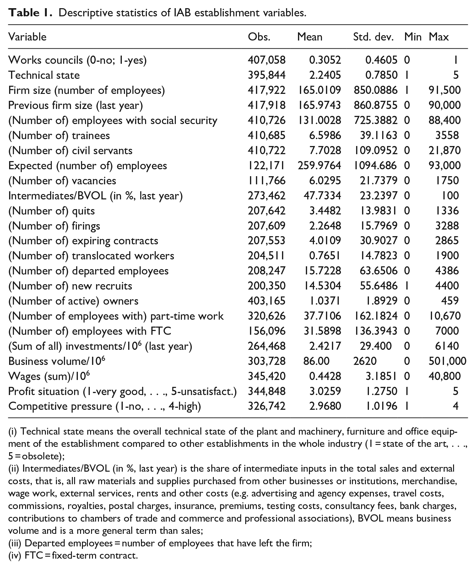
(i) Technical state means the overall technical state of the plant and machinery, furniture and office equipment of the establishment compared to other establishments in the whole industry (1 = state of the art, . . ., 5 = obsolete);

(ii) Intermediates/BVOL (in %, last year) is the share of intermediate inputs in the total sales and external costs, that is, all raw materials and supplies purchased from other businesses or institutions, merchandise, wage work, external services, rents and other costs (e.g. advertising and agency expenses, travel costs, commissions, royalties, postal charges, insurance, premiums, testing costs, consultancy fees, bank charges, contributions to chambers of trade and commerce and professional associations), BVOL means business volume and is a more general term than sales;

(iii) Departed employees = number of employees that have left the firm;

(iv) FTC = fixed-term contract.

Table 2.

Correlation coefficients of changes in the number of workers and other IAB establishment variables.

Variable	Corr. coef.	Variable	Corr. coef.
Investments	0.0386*	Number of expected workers	−0.1939*
Works council	−0.0101*	Number of vacancies	0.1395*
Part-time work	0.0152*	Share of business volume abroad	0.0161
Technical status	−0.0125*	Number of fixed term employees	0.0829
Quits	0.0114*	Working time accounts	−0.0071
Firings	−0.0802*	Employees with profit sharing (PS)	0.0061
Departed employees	−0.2061*	Number of high-skilled workers	0.0992*
New recruits	0.1356*	Employees with training	−0.0309*
Intermediates	0.0062*	Short time workers	−0.0416*
Wages	−0.0722*	Profit situation of the company	−0.0251*

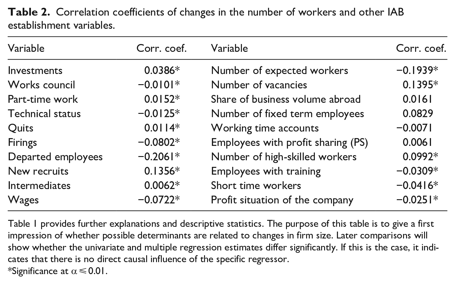
Table 1 provides further explanations and descriptive statistics. The purpose of this table is to give a first impression of whether possible determinants are related to changes in firm size. Later comparisons will show whether the univariate and multiple regression estimates differ significantly. If this is the case, it indicates that there is no direct causal influence of the specific regressor.

Significance at α ⩽ 0.01.

No theory can convincingly explain why some companies are more vulnerable to crises than others. It is also unclear why some of these firms only experience short-run difficulties in the face of a crisis. For other firms, the difficulties are substantial and cannot be resolved within just a few years.

The application of a variable selection method detects how many regressors should be selected without obtaining problems with multicollinearity, namely, too small variances of the estimation functions for the coefficients described by eigenvalues. However, this cannot speak much to which regressors are important from a substantial perspective. The literature suggests different variable selection procedures that do not lead to the same regressors, and no clear superiority of one method can be identified. Therefore, we chose different selection procedures. If they lead to a similar specification, we can interpret this as a good selection

We use three methods that can detect which variables are relevant and whose specifications are suitable – stepwise regression at pr (0.20) as the stopping rule (Bendel and Afifi, 1977), lars estimates (Efron et al., 2004) and a lasso approach (Belloni et al., 2012). These three procedures are described in Appendix 1. Table 3 shows that the selection methods lead to comparable results. Because the estimates of firm size change use data from various waves of the same establishments, cluster robust standard errors are applied in Tables 5 and 6.

Table 3.

Estimates of firm size changes based on regressor selection procedures – stepwise, lars and lasso.

Variable	Stepwise	Lars	Lasso
New recruits	0.7959	0.8999	0.8361
Firings	−0.2903	−0.2283	−0.1168
Quits	0.4813	0.3192	0.3980
Departed_employees	−0.8165	−0.9078	−0.8890
Investments/10⁸	−0.0621	−0.1285
Technical state	−1.5807	−1.5096	−1.3787
Works council	−0.3809	−0.6996
Wages/10⁶	1.2173	1.8181	0.5594
Part-time work	0.0067	0.0109	0.0210
Intermediates/business volume		0.0131
_cons	3.0692	2.4540	2.0394
N	104,400	78,289	131,360
r²	0.1582	0.1865	0.1659

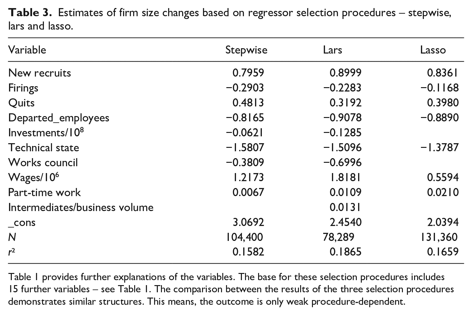
Table 1 provides further explanations of the variables. The base for these selection procedures includes 15 further variables – see Table 1. The comparison between the results of the three selection procedures demonstrates similar structures. This means, the outcome is only weak procedure-dependent.

In Tables 6 –10, we focus on the four major economic crises in Germany since 1993, where we have selected in Table 5 the years of the peaks of the crises: 2000, 2008, 2020, and 2022. However, this is ambiguous, and the designation of the four crises is by no means uniform in the literature. For example, it makes sense to denote the Ukraine War as an energy crisis, but the war is still ongoing, so we cannot be sure that 2022 was the peak year of the war. With respect to the change in firm size, we have a hint. As crises normally can span across multiple years and we are interested in the periods before and after the peak of a crisis, we present with Tables 7 –9 the estimates of 3-year intervals. Currently, we have to restrict this to the dot-com, financial, and COVID-19 crises because data for 2023 are still missing.

A problem with this approach is that the post-COVID-19 year overlaps with the year when the Ukraine War started. This is even more the case if the Ukraine War is not only counted from Russia’s invasion of Ukraine in 2022 but also if the annexation of Crimea 2014 is seen as the beginning of the war. The duration of the crises investigated also differed. Nevertheless, we model the crises in the same manner for reasons of comparability.

In addition, the dataset contains yearly data only. However, the crises do not start at the beginning of the year and do not end at the end of the year. Furthermore, an analysis based on individual data could be advantageous if we consider quit effects. This procedure has the disadvantage that company reactions cannot be identified.

Furthermore, it is difficult to detect whether any other unobserved influences are at play. Of course, in some cases, relevant variables are known and can be incorporated as dummies. To solve the problem with unobserved influences, panel estimators are applied. First, we test by Breusch and Pagan (1980) whether random effects exist. Second, if the answer is positive, then we should decide by the Hausman (1978) test whether the random or fixed effects approach is preferable.

Descriptive statistics and graphs

Table 1 presents the maximum number of observations for our relevant variables and the descriptive statistics. Of course, they differ from regression estimates. If we follow the development of the average firm size per year, measured by the number of employees, then no clear crisis-specific peculiarities can be seen. Possible explanations for this reduction may be decreasing fixed costs, increasing labour intensity, and increasing productivity, but further investigations are necessary.

Figure 1 describes the history of firm size changes since 1993. Here, we observe a different development. Initially, until 2004/05, negative changes were characteristic. However, the reduction is decreasing. From 2005 to 2006, positive changes are typical. Altogether, we can distinguish three phases: 1992/93–1997/98, 1998/99–2004/05, and 2005/06–2021/22. In phase 1, the positive development is stronger than that in the rest of the considered period. Phase 2 is characterised by a smooth course disrupted by 2000/01. In phase 3, the increase in the beginning is nearly the same as that in the end.

Figure 1.

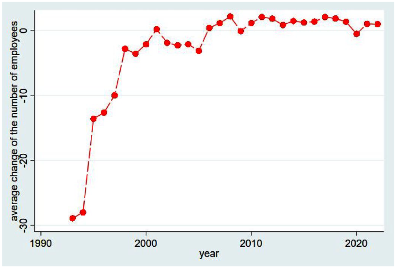
Average change of establishment size per year.

A simple and unique sorting from our identified crises to structural breaks in Figure 1 does not seem possible by the pure descriptive analysis. However, the peaks in Figure 1 signal movements in the dot-com and finance crises. The relatively low point of change in average firm size in 2019–2020 coincides with that in the first year of the COVID-19 pandemic. This means that the establishments were cautious in hiring, as the effects of COVID-19 were unknown. The overlap and compensation of different influences as well as insufficient phasing or the neglect of upstream and lagged effects could be reasons that only weak links are revealed. These suspicions need to be investigated.

The next two graphs provide a first impression of the influence of specific determinants on firm size movements. Figure 2 shows that the development of recruited and departed employees is similar but not the same. The latter would mean that the average size of an enterprise would not change if no other factors were effective. The real picture differs. Indeed, a decreasing tendency is characteristic, but the development is not completely parallel. In more years, the number of recruited workers exceeds the number of those who have left. This can be observed especially in recent times. Figure 3 shows the number of departed workers. Two partial components are considered, namely, quits by employees and layoffs by the firm. In nearly all years, the former is larger than the latter. The driving force is workers’ resignation and not dismissal by companies, as was the case in the past. Employees are thus in a stronger position than employers. Caution is advised when generalising this statement. In the next step, we ask whether potential determinants correlate with the change in the number of employees. The selection is based on determinants that are mentioned in the literature (see Section 2) and that follow statistical selection procedures – as described in the next section. The results are presented in Table 2. However, they are less informative for further selection, as they do not discriminate enough. Only a few significant linear relationships are shown.

Figure 2.

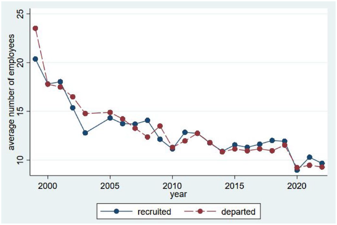
Average recruited and departed employees.

Figure 3.

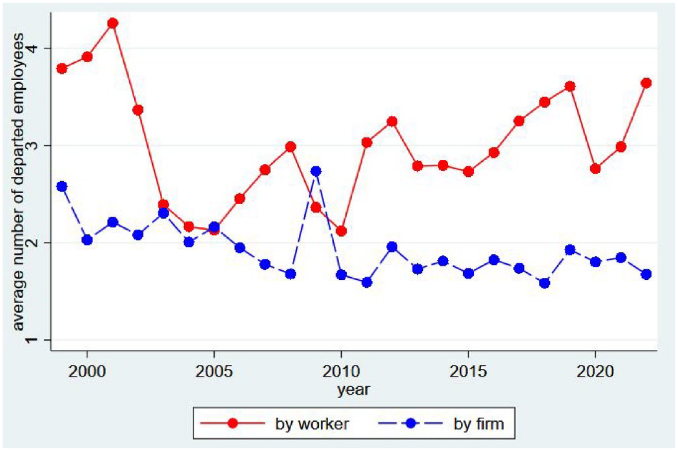
Average number of quits by workers or by the firm.

Furthermore, we could present more figures where the relationship is controlled under an additional influence, for example, by education, income, technical state, competitive pressure, or profit situation. The latter situation is presented in Figure 4. In the case of good to very good profitability, firm size and wage level are positively linked. In an unsatisfactory profit situation, the correlation is negative. We return to these points in the next section when multiple regressions are investigated. To achieve adequate handling of the profit situation in the multivariate analysis, we use Figure 4 as the base.

Figure 4.

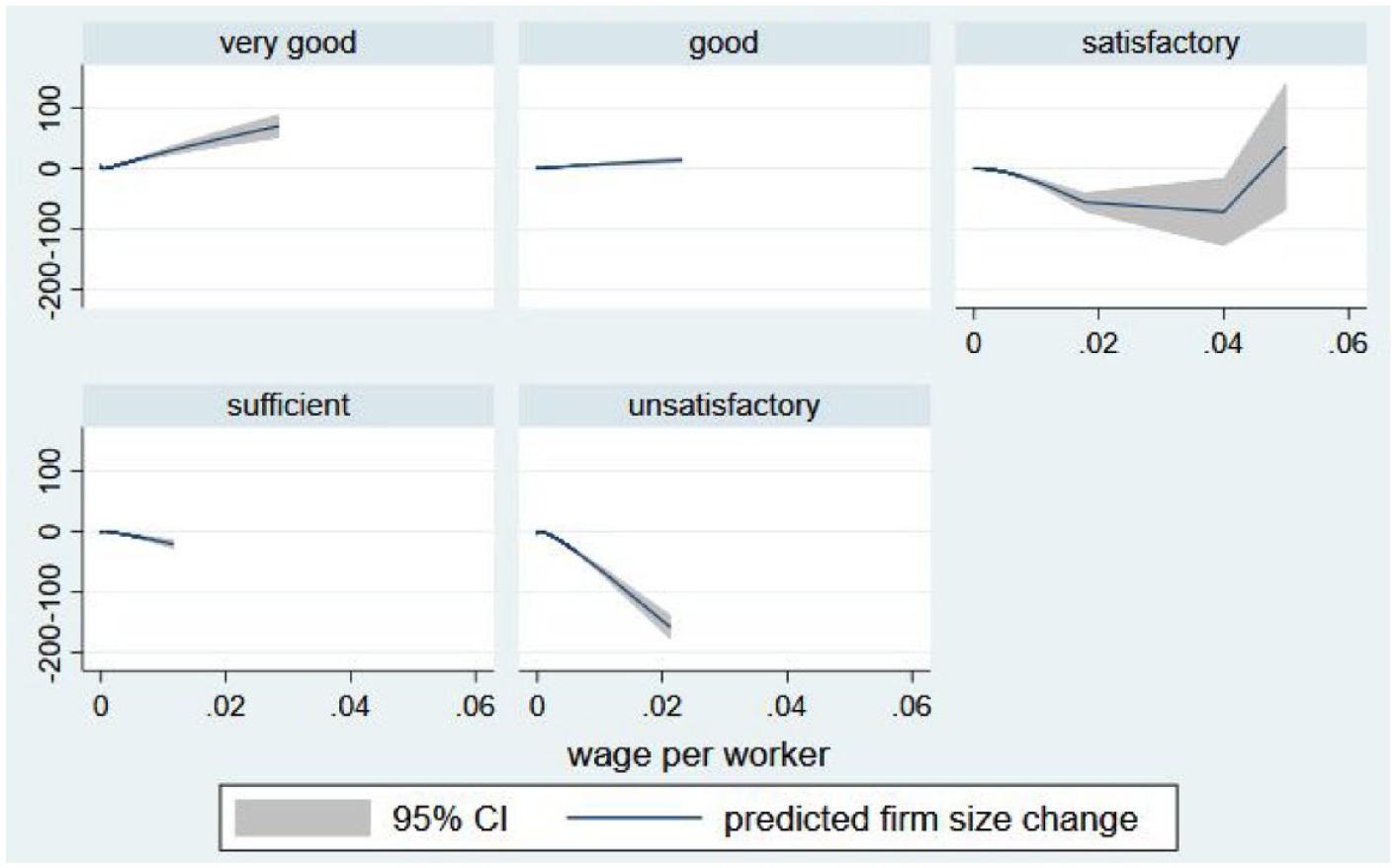
Average firm size change and wage per worker split by the profit situation.

Pooled regressions and panel estimates of firm size development

Table 3 shows the chosen regressors based on the three mentioned selection procedures: stepwise, lars, and lasso. The intention is twofold. First, we have a starting point for specific variables in Table 2. Second, we decided on the specifications for further investigations. The standard errors and significances are negligible at this stage. Fortunately, very similar variables are selected in Columns (1) to (3), Table 3. There is a clear ranking. The lars procedure selects more relevant variables than stepwise, and the latter selects more than lasso. This means that we can determine the lasso specification and the lars model. The stepwise specification represents a middle way. The preselection recommendation in Section 4 was successful, and our three selection procedures confirmed that the preselection was relevant – with one exception, namely, the ‘profit situation’. Disregarding ‘profit situation’ would be difficult, and the estimates in Columns (4) and (5) of Table 4 are further hints of these doubts; therefore, we find negative and significant effects. This finding is also in accord with theoretical expectations. Most likely, it would be better to split the ordered ‘profit situation’ variable into dummies, as shown in Figure 4.

Table 4.

Estimates of firm size changes with standard errors that are clustered at the establishment level of different specifications.

Variable	(1)	(2)	(3)	(4)	(5)
New recruits	0.8920***	0.8999***	0.8711***	0.6570***	0.6604***
Firings	−0.2822	−0.2283	−0.1846	−0.3597*	−0.3630*
Quits	0.2860	0.3192*	0.2642	0.3503	0.3343
Departed employees	−0.8607***	−0.9078***	−0.8665***	−0.7505***	−0.7501***
Investments/10⁸	0.0222	−0.1285		−0.0765	−0.0782
Technical state	−1.6512***	−1.5096***	−1.0221**	−0.9458*	−0.7920
Works council	−0.5202	−0.6996	−0.7134	−2.0390**	−2.027**
Wages/10⁷		0.1818	0.7236	0.4033**	0.4084**
Part-time work	0.0203	0.0109	0.0174	−0.0102	−0.0147
Intermediates	0.02093	0.0131	0.0154	0.0201	0.0114
No investments			−0.8237
Profit situation				−0.7456**	−0.7308**
Owner				0.0782	0.0309
Business volumes				−0.0121	−0.0248
FTC employees				0.2591**	0.2713**
Agriculture					−6.3087
Manufacturing					2.0107
Construction					3.5799
Trade					4.2145
Transport					4.9206
Services					0.2429
_cons	2.5848	2.4540	1.2985	−.2091	−1.8768
N	78,290	78,289	96,591	27,152	26,133
r ²	0.1834	0.1865	0.1806	0.3478	0.3519

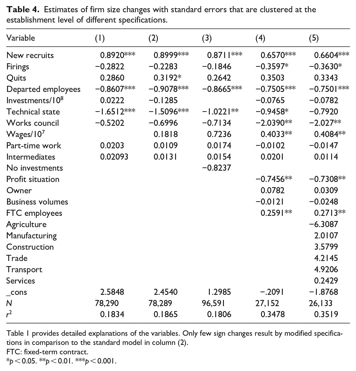
Table 1 provides detailed explanations of the variables. Only few sign changes result by modified specifications in comparison to the standard model in column (2).

FTC: fixed-term contract.

p < 0.05. **p < 0.01. ***p < 0.001.

We start with a mixture of the three selection procedures in Column (1) of Table 4. In contrast to the stepwise approach, the wage variable is not selected, and the intermediates variable of the lars approach is added. From the viewpoint of economic theory, wages are most important. Therefore, we compare the estimates in Column (1) with those in Column (2). Wages are insignificant, and the influence of the other determinants changes only moderately. New recruits and firings show the expected outcome, and these effects are in accordance with Hypothesis H1. We should stress that only the former variable is significant and that the effects are larger than those of the latter.

It seems surprising and does not support Hypothesis H3 that investments have no statistical influence, and this outcome does not change if the quantitative variable is substituted by a dummy, regardless of whether it is invested (see Column (3)).

A further extension in Columns (4) and (5), where regressors are added that are not indicated as relevant in Table 3, leads to some remarkable modifications. The number of observations varies between the columns and decreases as determinants are added that are not recorded in each wave. Now, wages are important for firm size changes. Firm sizes are larger for companies with high wages. This is plausible. The major modification in Columns (4) and (5) compared with Columns (1)–(3) is the introduction of the profit situation. A good profit situation has a positive direct effect on firm size (see also Figure 4) but also fosters the willingness of firms to pay higher wages, which may increase productivity.

The influence of works councils is also significant. They hinder pure expansion and foster internal development in accordance with Hypothesis H2. If this is not balanced, then the firms react with firings. This is more likely if the economic situation is generally bad. We find this confirmed in Columns (4) and (5). Firing is now negatively significant in the estimation. Finally, we should emphasise that no industry effects could be detected and that fixed-term contracts (FTC) play a visible role. The more companies can enforce fixed-term contracts, the more they tend to expand, as they have more possibilities to adapt to changing situations.

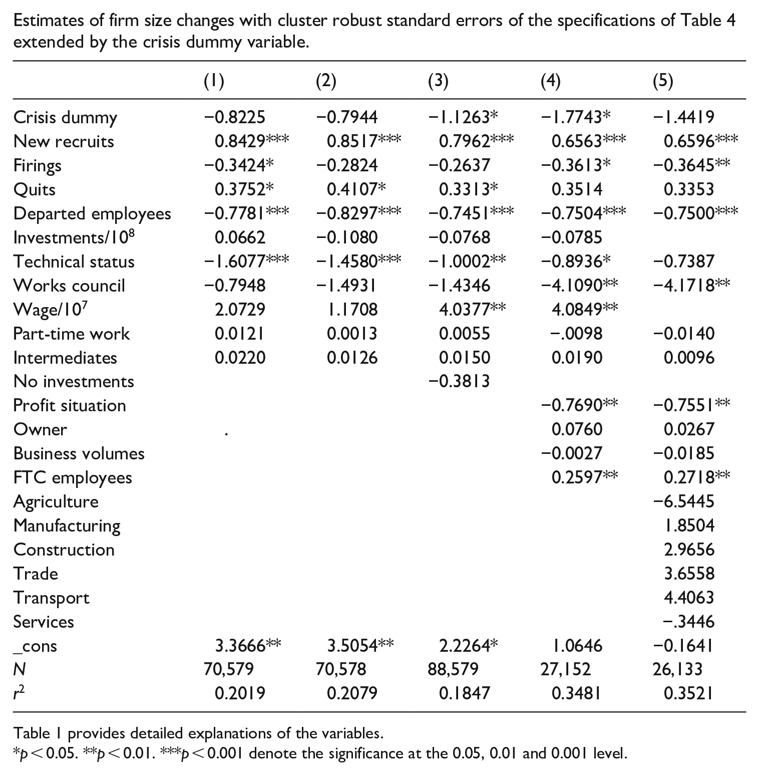
The results presented in Table 4 do not contain specific crisis information. Therefore, due to our major interest we extend the specification with the crisis dummy. This idea is followed in Appendix 2. The results show that in crisis periods, average firm sizes are smaller than in non-crisis years. However, only in Columns (3) and (4) do we find a significant effect. This unsatisfactory result may be due to delayed adjustments by some firms and early adjustments by other firms. We experimented with other variables containing crisis information, namely, dummies of one specific crisis or up to three of the four crises, or annual dummies from 1999 until 2022. However, no systematic pattern could be identified.

Turning to Table 5 our results reveal a positive impact of hiring on firm size during all crises and normal times. In contrast, firings exhibit negative signs during the dot-com bubble, the financial crisis and the war against Ukraine as well as during normal times, whereas quits show negative coefficients, but insignificant effects during the financial crisis and the war against Ukraine. The number of departed employees always exerts a negative impact. Thus, the impact of the crises considered reveals their distinct effect in terms of firings and quits on the firm size as postulated in Hypothesis H1.

Table 5.

Estimates of firm size changes for four economic crises and crisis-free years with standard errors that are clustered at the establishment level.

Variable	Dot-com	Finance	Corona	Ukraine war	Crisis-free
	2000	2008	2020	2022	Periods
New recruits	0.8417***	0.6772***	0.5847***	0.4979***	0.8999***
Firings	−0.0868	−0.7510***	0.0870	−0.8478***	−0.2283
Quits	0.6940***	−0.0996	0.3875***	−0.2085	0.3192**
Departed employees	−0.9317***	−0.3176***	−0.7602***	−0.2963***	−0.9070***
Investments/10⁸	0.1314**	0.4473***	−0.4933***	−0.2107***	−0.1286
Technical state	−2.4016	−5.3852***	−1.2213***	−1.1270***	−1.5096***
Works council	−0.4324	−0.1555	0.6324	1.2098	−0.6996
Wages/10⁶	−0.4960	−1.4650***	3.2242***	1.2694***	1.8181
Part-time work	−0.0558***	0.0279***	0.03011***	0.0108***	0.0109
Intermediates	0.0084	0.0344	0.0170	0.0055	0.0131
_cons	5.4104	10.8703***	1.1753	4.5562***	2.4540
N	3448	3169	3010	2710	78,289
r ²	0.2173	0.3898	0.3684	0.1505	0.1865

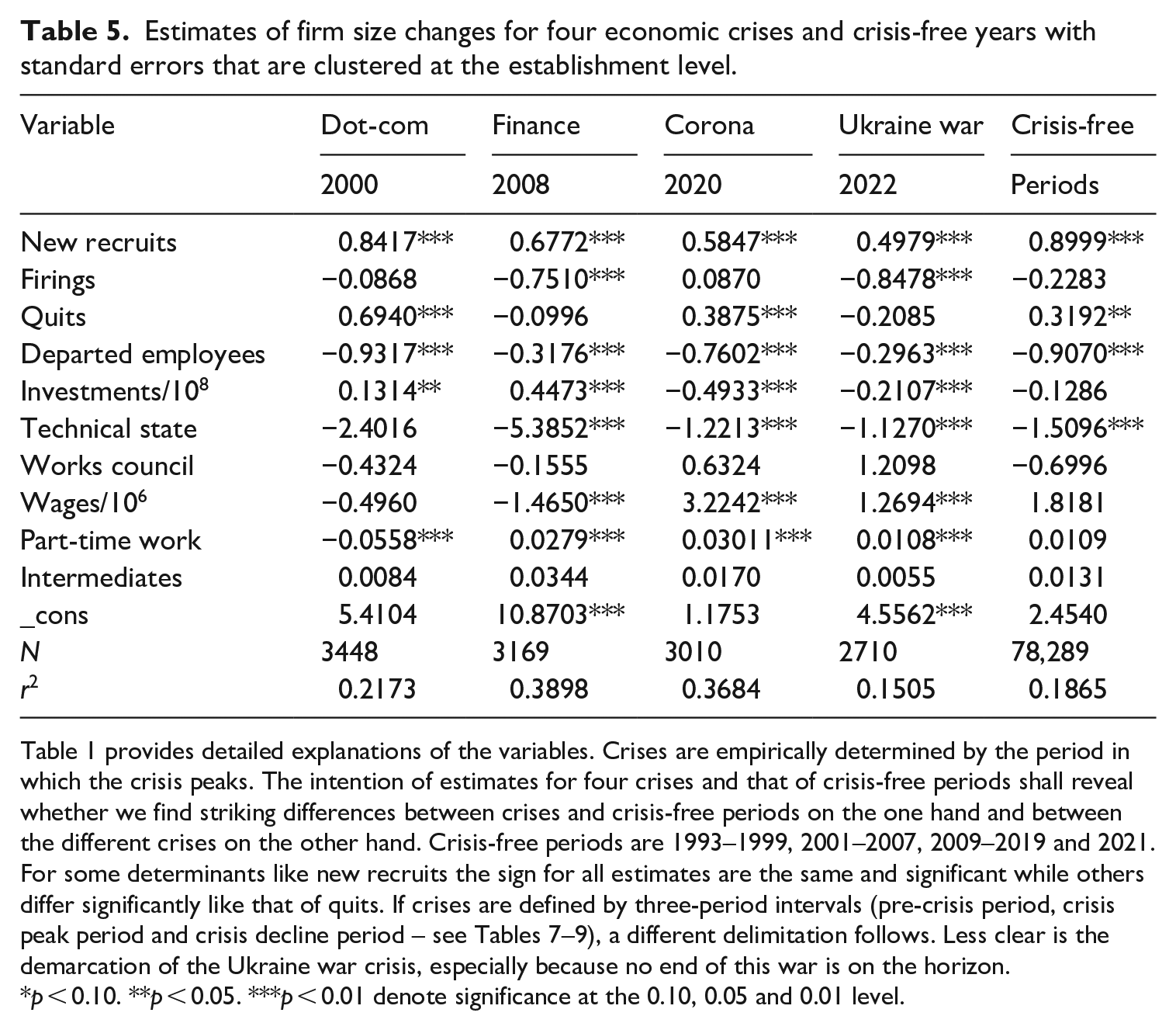
Table 1 provides detailed explanations of the variables. Crises are empirically determined by the period in which the crisis peaks. The intention of estimates for four crises and that of crisis-free periods shall reveal whether we find striking differences between crises and crisis-free periods on the one hand and between the different crises on the other hand. Crisis-free periods are 1993–1999, 2001–2007, 2009–2019 and 2021. For some determinants like new recruits the sign for all estimates are the same and significant while others differ significantly like that of quits. If crises are defined by three-period intervals (pre-crisis period, crisis peak period and crisis decline period – see Tables 7 –9), a different delimitation follows. Less clear is the demarcation of the Ukraine war crisis, especially because no end of this war is on the horizon.

p < 0.10. **p < 0.05. ***p < 0.01 denote significance at the 0.10, 0.05 and 0.01 level.

The results presented in Table 4 also corroborate Hypothesis H2 as the existence of works councils exerts a negative and significant influence but only if we control for wages and the profit situation.

Table 5 shows that the impact of investments on the firm size was negative only during the corona pandemic and the war against Ukraine; these results are in line with Hypothesis H3. In contrast and rejecting Hypothesis H3 partially during the dot-com bubble and the financial crisis the impact of investments was positive.

Our estimates show (Table 5) that part-time work and firm size development were negatively correlated during the dot-com crisis. In the other three crises, a reverse link was observed. Furthermore we find a positive relationship between wages and firm size during COVID-19 and the Ukraine War. For the other two crises, no effect or a negative effect could be identified.

In Table 6, in contrast to the pooled estimations in Table 4, unobserved heterogeneity is considered:

y_{l t, t - 1} = {x_{l t}}^{'} β + α_{l} + ε_{l t, t - 1}

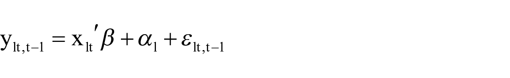
where l = 1, . . ., L are establishments, t = 1, . . ., T are the considered periods. The regressand y_lt,t-1 measures the change of establishment size between period t and t − 1. The regressors x_lt follow those from Table 4, column (2). Unobserved establishment heterogeneity is captured by α_l. That is potentially correlated with observed regressors x_lt (fixed effects model). The error term ε_lt,t-1 is assumed independent, identical distributed (iid).

Table 6.

Fixed effects estimates of firm size changes with standard errors that are clustered at the establishment level.

Variable	(1)	(2)	(3)	(4)
New recruits	0.7812***	0.5394**	0.9802**	0.9488**
Firings	−0.4201**	−1.0297***		−0.1383
Quits	0.2737	−0.2685		−0.8150
Departed employees	−0.6090***		−0.5278***
Investments/10⁸		−0.3389	−0.3060***	−0.3090***
Works council		0.2643	−0.1170	−0.2532
Part-time work		0.1313**	0.2222	0.2159
Technical state		−0.2223	−1.4780	−1.5017
Intermediates		0.0034	−0.0187	−0.0348
Wages/10⁷		0.3627*	0.4904**	0.5426***
Vacancies			0.5010*	0.5623**
Competitive pressure			−0.2379	−0.1995
Working time accounts			0.0059	0.01377
_cons	−2.2039	−11.4421***	−20.6064*	−25.6217*
N	152,650	78,289	18,524	18,524
r ²	0.1047	0.0897	0.2810	0.2408
Breusch-Paganχ²	20,180.31***	9330.10***	1428.47***	1378.10***
Hausmanχ²	2379.18	1249.26***	246.35***	238.03***

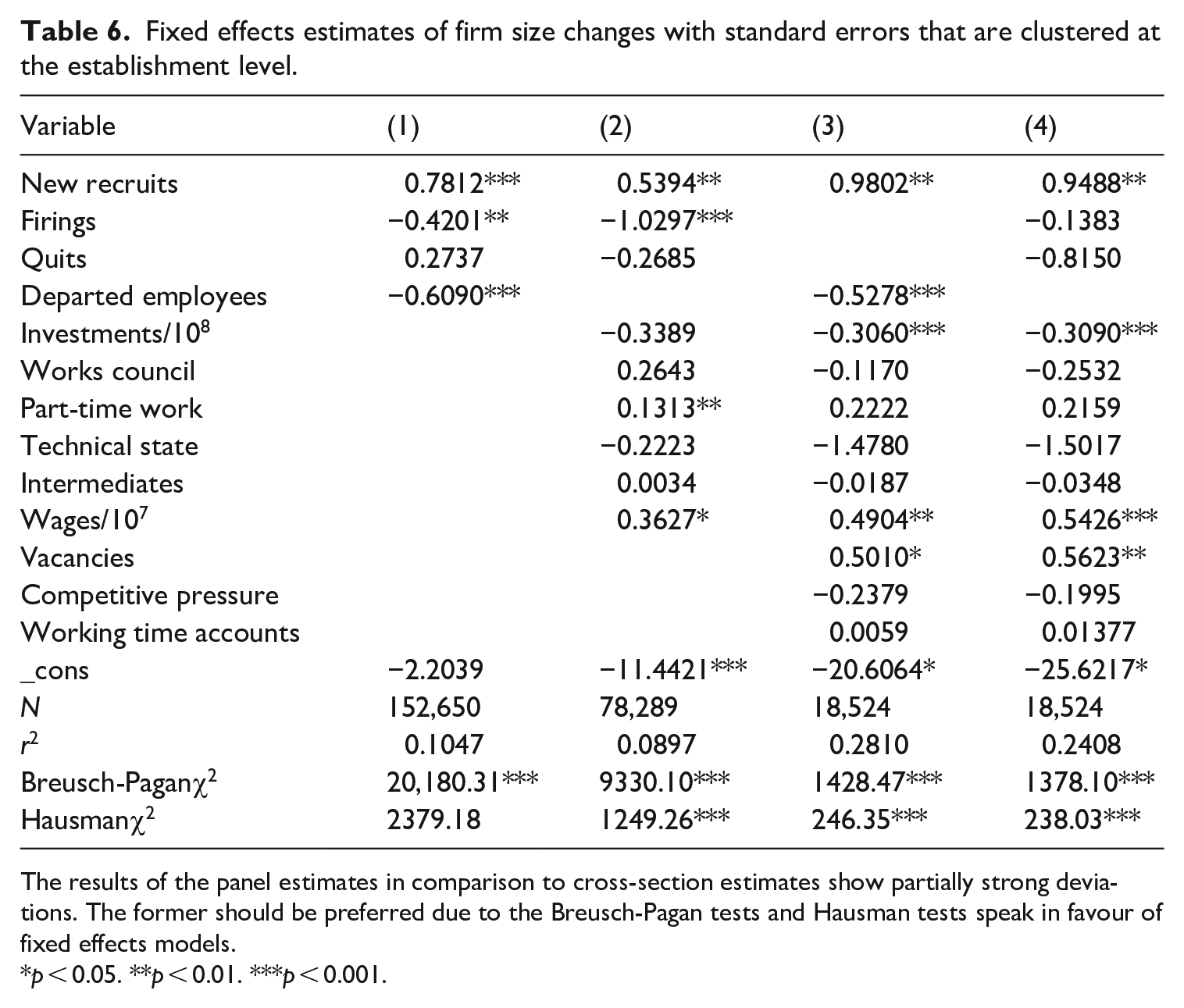
The results of the panel estimates in comparison to cross-section estimates show partially strong deviations. The former should be preferred due to the Breusch-Pagan tests and Hausman tests speak in favour of fixed effects models.

p < 0.05. **p < 0.01. ***p < 0.001.

The Breusch-Pagan test for random effects demonstrates an advantage of panel over pooled estimates. H₀, which states that no unobserved random effects, is rejected. The Hausman specification test rejects H₀, which states that unobserved firm effects are random. This speaks in favour of a fixed effects model. However, we should stress that the Hausman test has no systematic power against the alternative, and we cannot be sure that the unobserved establishment effects are time-invariant. If further regressors are added, the statistical advantage of fixed effects models becomes less important, and the χ² value falls (see line Hausman). That is why we are presenting both estimates, the random and fixed effects estimates, also simply to clarify the differences.

Column (2) of Tables 4 and 6 include nearly the same regressors. Insofar, a comparison is feasible. One difference should be stressed. The panel estimates show nonsignificant quit effects. A brief look at the signs of Table 4, Column (2) and Table 6 (2) shows that the signs differ for ‘quits’ and ‘works council’. This may be due to the missing ‘departed employees’ in Table 6 (2). For this reason, we present in Appendix 3 the panel estimates where ‘departed employees’ are included. A comparison with Table 6 (2) shows that the quits coefficient is now positive. The works council coefficient remains positive for the fixed effects, in contrast to the random effects estimation. In addition, no fundamental disparities can be observed.

Tests and specific effects around economic crises

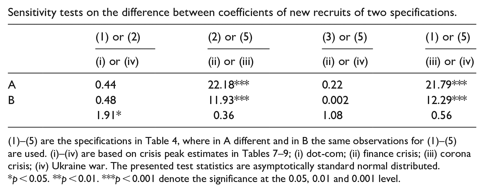
We have carried out different sensitivity tests (Hübler, 1989: 122). In a first step the analysis is restricted to the most important regressor, ‘new recruits’ (Appendix 4), where we distinguish in the upper part between models with constant and different observations in (1) to (5). In most comparisons, we find no significant differences. The comparisons between (1) and (5) and between (2) and (5) are exceptions. This is true for models with varying and constant observations.

In the lower part of Appendix 4, estimates of the four crises are compared, where for the dot-com, financial, and COVID-19 crises, the year with the peak of the crisis and for the Ukraine War, estimates of 2022 are used, the year in which the Ukrainian War began. No significant differences could be identified with respect to new recruits. Only the comparison between the dot-com crisis and the year of Russia’s invasion of Ukraine showed a statistically weak correlation. This speaks in this case in favour of dissimilarity of the two crises.

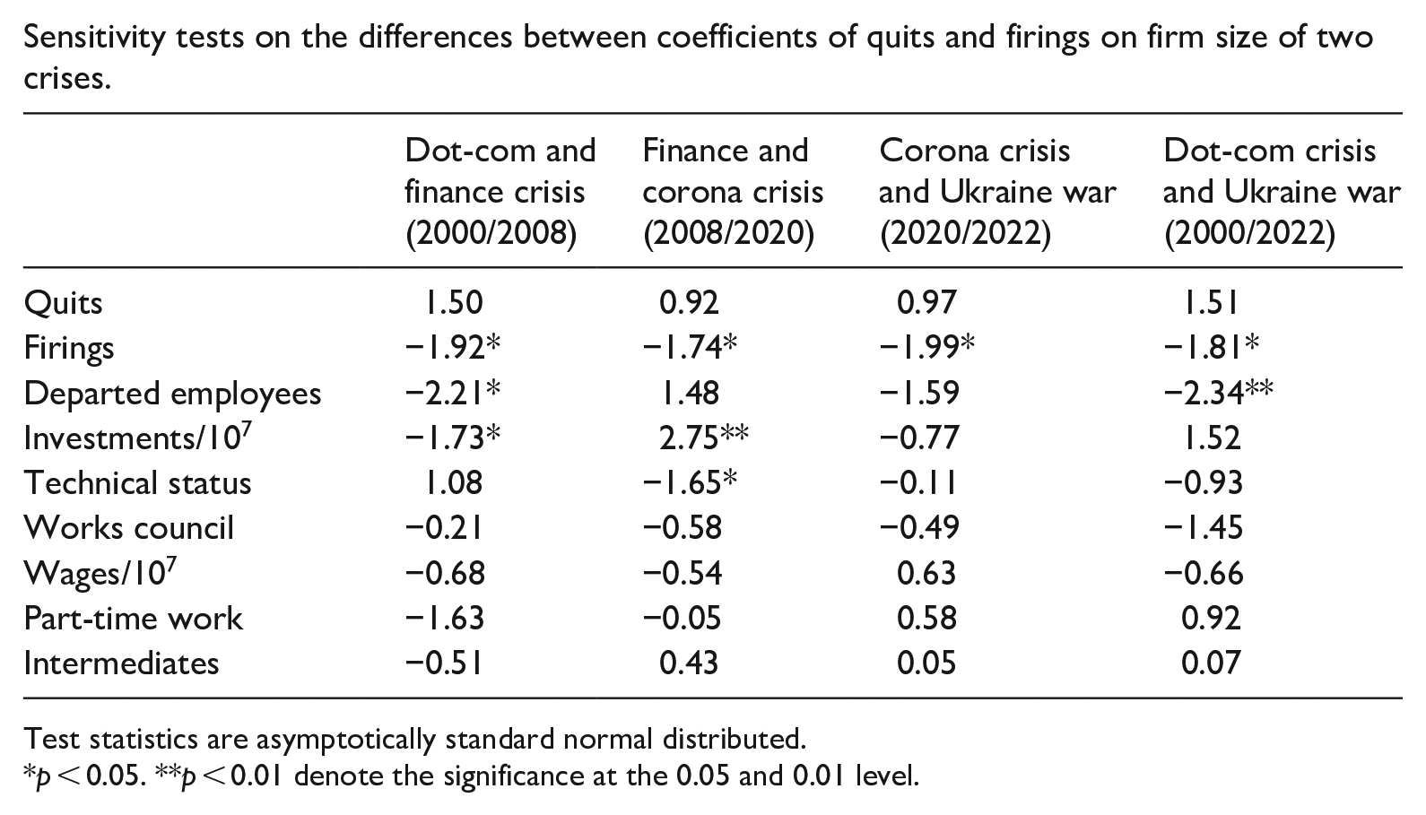
Focussing on the effects of quits and firings instead of new recruits leads to other conclusions. For successive crises, we do not find significant effects of quits on firm size, while firings induce weakly significant and negative firm size changes, as sensitivity tests show (Appendix 5, line quits and firings).

We also check whether the influence of other determinants on the change in firm size differs significantly between two crises. In most cases, the null hypothesis of equality (H₀) cannot be rejected. However for departed employees the comparison between the dot-com bubble in new economy companies and the finance crisis shows significant differences. The same could be detected between dot-com and the Ukraine War. Differences can also be identified with regard to investments. Here between the financial crisis and the dot-com crisis on the one hand and between the financial crisis and the COVID-19 on the other.

In Table 5, we look for peculiarities in the development of firm size before and during the major phase of the four economic crises based on specification (2) of Table 4. Although the magnitudes and origins of the crises are different, the relationships between some components and firm size are similar. The importance of new recruits for firm size development seems linked over the whole period.

The relevance of firings and quits varies more strongly between crises. During the financial crisis and the Ukraine War, firings affected firm size changes, while no clear links were revealed by quits. The opposite is evident during the dot-com and COVID-19 crises. During these phases, the effects of the quits are obvious. The significance of layoffs, on the other hand, is not apparent.

It would be too broad to claim that all the crises are generally close in their impact. Rather, the distinction between monetary financial market transactions and economic policy-induced goods market movements speaks more in favour of locating the dot-com and financial market crises more closely together. Conversely, the effects of the COVID-19 crisis and the Ukraine War should be more similar. We find that this is confirmed only by the influence of new recruits. Other differences must be effective. For example, the COVID-19 lockdown did not allow the continuation of national production. A relocation abroad was not as easily possible in the short run. Problems with energy delivery and the import of other raw materials due to sanctions against Russia in response to the war of aggression against Ukraine have led to bottlenecks in the import of raw materials. In this respect, the problem is similar. However, there are significantly more options than with the lockdown, even if not in the very short term. The financial crisis also did not provoke the same reactions as the dot-com crisis. Not all businesses and people in Germany have suffered from the dot-com crisis. In addition, others who were not involved in speculative transactions or believed that the problems could be overcome in a short time had positive expectations. Moreover, the quality and number of public subventions differed between these two difficult economic phases. Optimistic expectations are probably accompanied by expansive activities and an increase in firm size. Further business and personnel measures may follow changes in the purchasing policy, at part-time work or at the pressure of work councils to improve the working conditions of employees.

In Column (5) of Table 5, we have added estimates with the same specifications as in Columns (1) to (4) but restricted to crisis-free years. Therefore, we can see not only the differences between the crises but also in comparison to during normal economic times. Interestingly, Column (5) shows less significant influences than Columns (1) to (4). However, for most determinants, the sign of the estimated coefficients is the same for all five columns. This suggests that cyclical fluctuations are not dominant, but the general relationship is more important. Fundamental discrepancies are observed for investments, wages and part-time work. In normal times, investments do not seem relevant for firm size changes, while innovations during the dot-com crisis and the Great Recession signal positive development so that firms are ready to expand. During COVID-19 and the Ukraine War, the situation was too uncertain to answer with an increase in firm size. The negative coefficient in Columns (3) and (4) may show that investments aim more at restructuring to save costs. In a similar direction, we can argue that the wage reduction and downsizing of the company go hand in hand. Finally, the estimates reveal that part-time work and firm size are uncorrelated in crisis-free times, while especially during COVID-19, an expansion of part-time work led to an expansion of the company.

One central statement of our results is that a simple outcome transfer from one crisis to a new one is dangerous. Nevertheless, we should also look for parallels. One possibility is to compare the course of crises. We can do this with Tables 7 –9, where estimates of 3-year intervals are presented. They show that the average firm size not only increases with new recruits but also decreases with the number of departed employees during the peak of all crises but also before and after. This tendency holds true for the entire period under consideration. For the Ukraine War, we restrict our analysis to the year 2022 because there is no end in sight, and more recent data are still missing. The estimates can be found in Table 10. In comparison to Column (2) in Tables 7 –9, we find less clear results.

Table 7.

Estimates of firm size changes with standard errors that are clustered at the establishment level in the course of the dot- com crisis (1999–2000–2001).

Variable	Pre-crisis	Crisis peak	Crisis decline
New recruits	0.8962***	0.8417***	0.7719***
Firings	−0.5383***	−.0868	0.2564
Quits	0.1056	0.6940***	0.8521***
Departed employees	−0.7656***	−0.9317***	−0.8157***
Investments/10⁸	−0.3644***	0.1314**	−0.3070***
Technical state	−4.1382**	−2.4016	−3.1588***
Works council	0.1285	−.4324	−.2553
Wages/10⁷	−0.3060***	−.0496	0.0918**
Part-time work	−0.0275*	−0.0558***	−0.0249**
Intermediates	0.0099	0.0084	0.0136
_cons	10.6385**	5.410	5.6877*
N	2431	3448	4201
r ²	0.3383	0.2173	0.2020

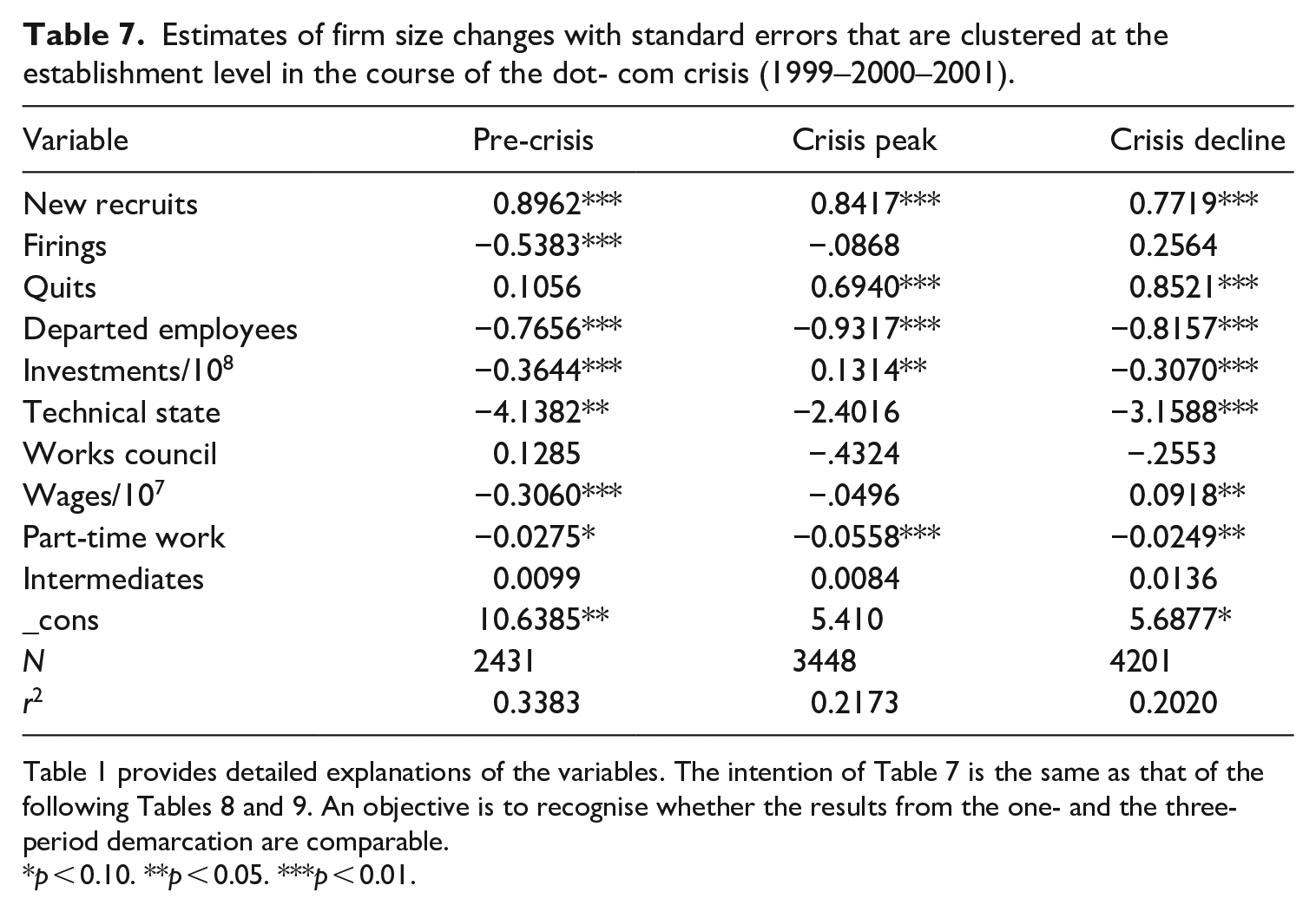
Table 1 provides detailed explanations of the variables. The intention of Table 7 is the same as that of the following Tables 8 and 9. An objective is to recognise whether the results from the one- and the three-period demarcation are comparable.

p < 0.10. **p < 0.05. ***p < 0.01.

Table 8.

Estimates of firm size changes with standard errors that are clustered at the establishment level in the course of the finance crisis (2007–2008–2009).

Variable	Pre-crisis	Crisis peak	Crisis decline
New recruits	0.7228***	0.6772***	0.8579***
Firings	−0.7826***	−0.7510***	−0.9580***
Quits	1.3523***	−0.0996	−0.2730
Departed employees	−0.8219***	−0.3176***	−0.6558***
Investments/10⁷	0.0447	0.4473***	−0.9390***
Technical state	−2.5744	−5.3852***	−0.2666
Works council	−2.8302	−0.1555	−3.0893
Wages/10⁷	−0.5428	−0.1465***	0.1378***
Part-time work	0.0494***	0.0279***	−0.0350***
Intermediates	0.0049	0.0344	−0.0266
_cons	7.0308	10.8703***	1.7201
N	3084	3169	2529
r ²	0.2069	0.3898	0.1506

Table 1 provides detailed explanations of the variables. Compare with Tables 7 and 9.

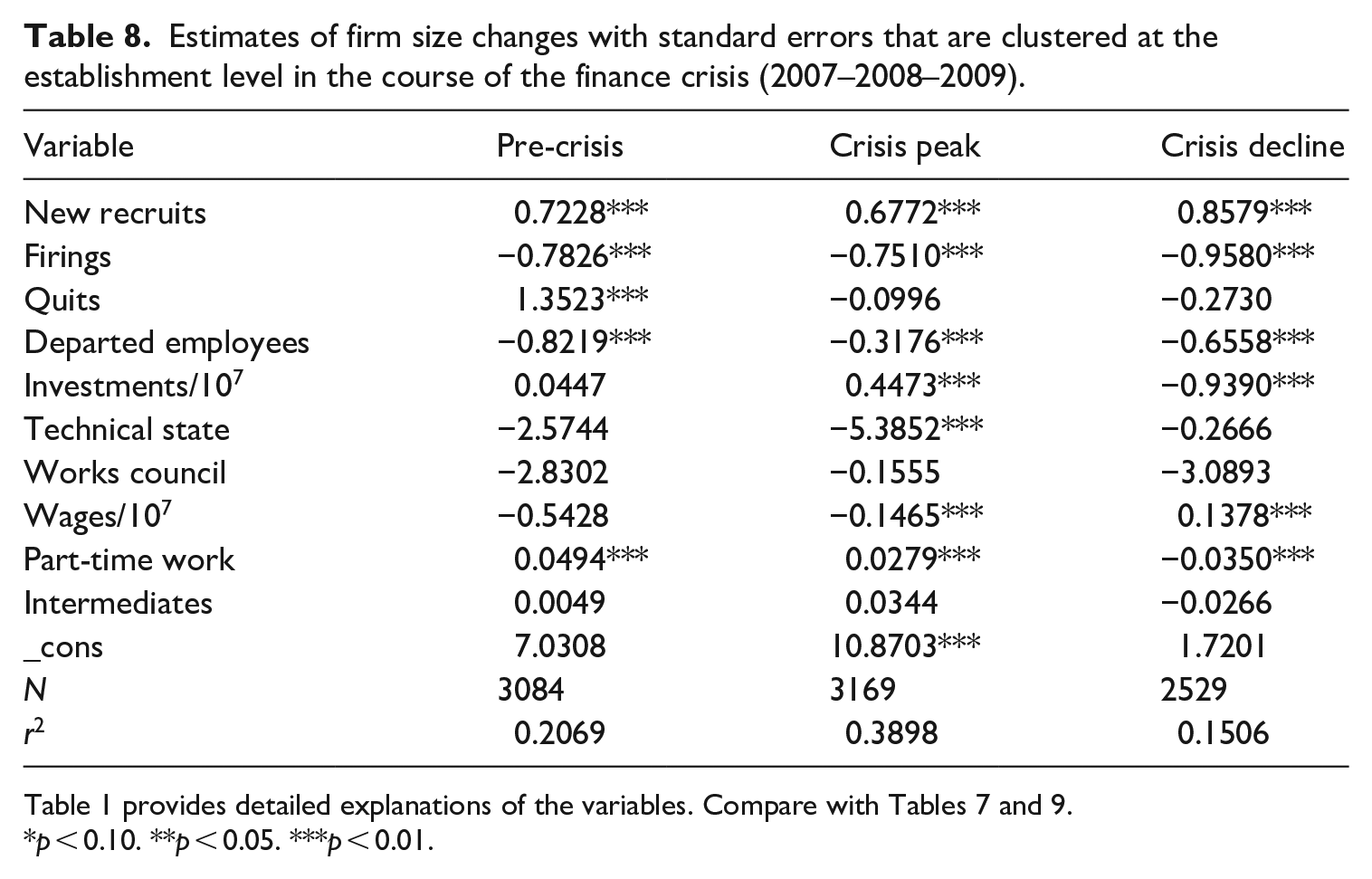
p < 0.10. **p < 0.05. ***p < 0.01.

Table 9.

Estimates of firm size changes with standard errors that are clustered at the establishment level in the course of the corona crisis (2019–2020–2021).

Variable	Pre-crisis	Crisis peak	Crisis decline
New recruits	0.1476**	0.5847***	1.0583***
Firings	−0.3051*	0.0870	−1.0182***
Quits	0.1150	0.3875***	−0.4947***
Departed employees	−.0825	−0.7602***	−0.4191***
Investments/10⁷	−0.5483***	−0.4933***	0.7233****
Technical state	−1.8425***	−1.2213***	−1.0556
Works council	−1.0382	0.6324	−1.4434
Wages/10⁷	0.4779**	0.3224***	−0.4308***
Part-time work	0.0660***	0.0301***	0.0036
Intermediates	0.0084	0.0170	0.0111
_cons	3.7987***	1.1753	1.6490
N	3499	3010	2581
r ²	0.2177	0.3684	0.8092

Table 1 provides detailed explanations of the variables. Compare with Tables 7 and 8.

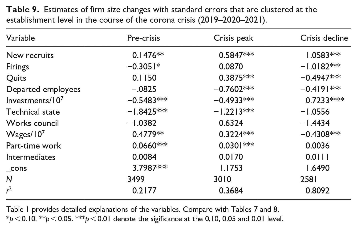
p < 0.10. **p < 0.05. ***p < 0.01 denote the sigificance at the 0,10, 0.05 and 0.01 level.

Table 10.

Cluster robust estimates of firm size changes with standard errors that are clustered at the establishment level of the Ukraine War (2022).

New recruits	0.4279*
Firings	−0.8478*
Quits	−0.2085
Departed employees	−0.2963
Investments/10⁷	−0.2107
Technical status	−1.1270*
Works council	1.2098
Wages/10⁷	0.1269
Part-time work	0.0108
Intermediates	0.0055
_cons	4.556*
N	2710
r ²	0.1505

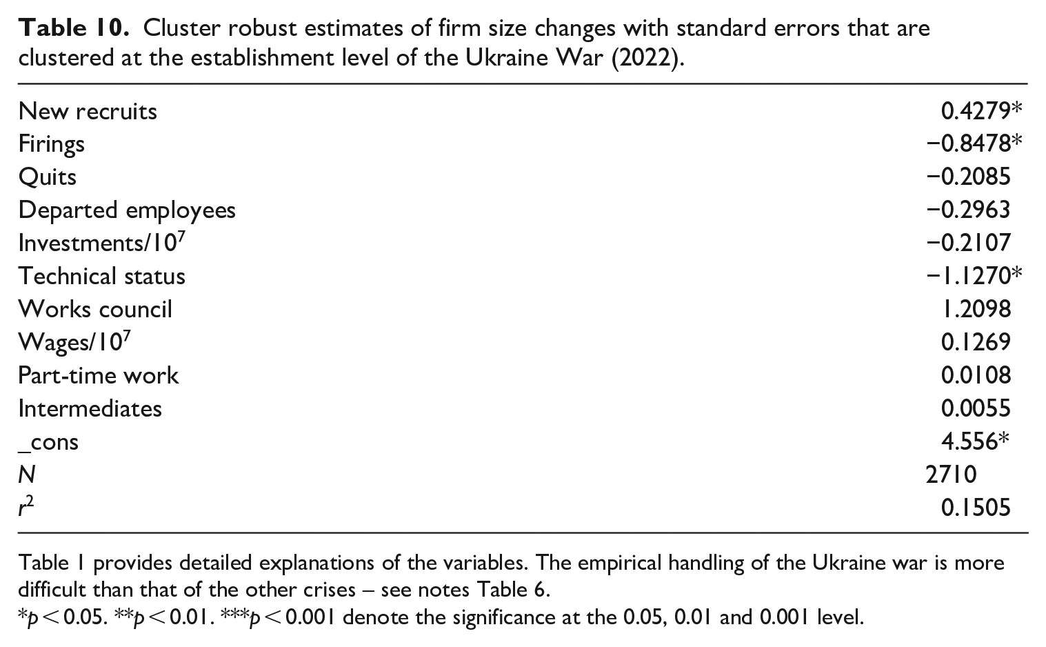
Table 1 provides detailed explanations of the variables. The empirical handling of the Ukraine war is more difficult than that of the other crises – see notes Table 6.

p < 0.05. **p < 0.01. ***p < 0.001 denote the significance at the 0.05, 0.01 and 0.001 level.

Differences are observed in the strength of the effects before and after the peak of the crisis, expressed by the coefficients. The course of average firm size change with respect to hired workers can be described as continuous over the 3-year interval during the dot-com and COVID-19 crises. A more discontinuous pattern is typical in the Great Recession, not only with respect to new recruits but also with respect to departed workers. If we split between the components quits and firings, then only the latter shows significant differences between two crises (Appendix 5, line quits and firings). Sensitivity tests are also carried out for other relevant regressors in Tables 6 –10. Almost no test among the comparisons considered between two crises reveals clear differences.

We could also present estimates for crisis-free times analogous to those in Column (5) in Table 5 if crises are described as 3-year intervals. A distinction, which is not shown in the Tables, is a change in signs in comparison to Column (5) of Table 5 for firings, but this result is insignificant. Furthermore, we can also mention that the effects of quits and that of the technical state on firm size are only insignificant when crises are characterised by an interval length of 3 years. This suggests that a 1-year description of crises is more informative.

Conclusion

Using 30 waves and approximately 418,000 observations of the German IAB Establishment Panel Survey 1993–2022, we analyse the relationship between firm size adjustments, job mobility, industrial relations, and technology adoption during four economic crises (the dot-com, financial, and COVID-19 crisis, and the Ukraine War) and normal times. Additionally, we consider whether differences exist between firms of different sizes affiliated with various economic sectors and the profit situation as well as unobserved time-invariant effects. Although our main focus of interest lies on the impact of hiring and layoff variables on the dynamics of firms’ size over four major crises in the last 30 years, we investigate the influence of additional variables such as the existence of works councils, investment, profit situation, wages, qualification and part-time work as well as unobserved heterogeneity.

Our descriptive analyses provide fresh insights into the sharp decline in average firm size during the 1990s and the moderate development of the last two decades. During times of an economic crisis, the effects are greater than during normal times. The differentiation of the number of workers departed by employee quits and firm layoffs demonstrates that in nearly all years, the former is larger than the latter. According to our panel estimations, the impact of hiring on firm size is always significant and positive. In contrast, firings exhibit a negative and during the dot-com bubble and the corona crises as well as during normal times insignificant effect. Whereas quits only show negative effects during the financial crisis and the war against Ukraine, the number of departed employees always exerts a negative firm size effect Investments reduce the average firm size. Not surprisingly, the state of the technology does not always have significantly negative effects, which is evidence of internal adjustment. The existence of a works council exerts a negative and significant influence only if we control for wages and the profit situation. The development of part-time employment has a positive impact during the Great Financial Crisis, the COVID-19 pandemic as well as the war against Ukraine.

Furthermore, comparisons between the different crises are of interest: for example, for departed employees the comparison between the dot-com bubble and the financial crisis reveals significant differences. The same could be detected between dot-com and the Ukraine War. Differences can also be identified with regard to investments. Here between the financial crisis and the dot-com crisis on the one hand and between the financial crisis and the COVID-19 on the other.

Thus, our panel estimates only partially corroborate the results gained from previous studies but confirm our hypotheses and, therefore, provide valuable insight.

With respect to not only the variables discussed thus far but also others, our results reveal that a simple transfer from one crisis to a new one may be dangerous. However, interesting parallels are also visible. For example, during the whole observation period, the average firm size increases due to new recruits and decreases due to the number of departed employees during the peak of all crises but also before and after. Thus, our analyses imply that the economic crises investigated reveal similarities in the sense that the relevant variables exert similar effects, but some differences are also observable. Interestingly, the general trend of declining firm size is more pronounced during crises, followed by a rebounding effect after crises.

Footnotes

Appendix 1: Stagewise,lars and lasso as variable selection procedures

Stepwise regression (stagewise) evaluates each variable in turn on the basis of its significance level and accumulates the model by adding or deleting variables sequentially. All the variables ultimately included that have F statistics larger than four. It is hardly appropriate to call these F statistics and base inference on them as if they are drawn from an F distribution. There is no clear stopping rule to be used in practice. Bendel and Afifi (1977) present different stopping rules and under which condition they are optimal. Within this range lies p = 0.2 that is used in our investigation. It is known a priori that they all will be larger than four. From this reason it makes sense to avoid stepwise regression methods (Greene, 1997: 401). There are further numerous criticisms of stepwise regression, one of which is that it is a ‘greedy’ algorithm and that the regression coefficients are too large. Conventional forward stepwise regressions are too strongly focused on the prediction accuracy.

Furthermore, least angle regression (lars) is applied, a method developed by Efron et al. (2004). A parsimonious set of the available covariates is selected for the efficient prediction of response variables. Few steps are required. The procedure begins with all coefficients being set equal to zero and identifies the predictor most correlated with the response variable, say x₁. The largest step in the direction of this predictor is taken until some other predictor – say x₂ – has an equal amount of correlation with the current residual u₁. Lars proceeds in a direction equiangular between the two predictors, x₁ and x₂, until a third predictor, x₃, earns its way into the ‘most correlated’ set. This mechanism is demonstrated by the following graph where μ = Xβ and y̅_k (k = 1,2,3,. . .) are averages of the endogenous variable

Lars proceeds equiangularly among x ₁, x₂ and x₃, that is, along the ‘least angle direction’ until a fourth variable, x₄, enters, and so on. The Cp criterion

$C_{p} (μ) = (| | y - μ | | / σ^{2}) - n + 2 d f μ σ^{2}$

is used as the stopping rule, where σ² is the residual variance and df = Σcov(μ,y)/σ² are the degrees of freedom. The procedure stops, no more regressors are incorporated, if Cp is smallest. Cp is an unbiased estimator of prediction error. Insofar Cp minimization is trying to be an unbiased estimator of the optimal stopping point. Perhaps, the stopping rule can be improved if the df multipier 2 in Cp is increased.

The Least Absolute Shrinkage and Selection Operator (lasso), developed by Tibshirani (1996), has also a parsimony property. The estimation is based on

$\hat{β} = a r g m i n {Σ_{i}}^{N} {(y_{i} - {Σ_{j}}^{p} x_{i j})}^{2} s u b j e c t t o {Σ_{j}}^{p} | β_{j} | < = t$

where t(⩾0) is a tuning parameter. We follow Belloni et al. (2012). This robust lasso approach allows an estimation under heteroscedastic non-Gaussian and clustered disturbances (rlasso)

$\hat{β} = a r g m i n m i n {Σ_{i}}^{N} {(y_{i} - {Σ_{j}}^{p} x_{i j} b_{j})}^{2} + λ {Σ_{i}}^{p} | b_{j} | ϒ_{j}$

where λ > 0 is the ‘penalty level’ and ϒ_j are the ‘penalty loadings’.

This procedure selects fewer significant variables than lars. A problem with rlasso remains also the pre-selection of variables. It has an influence on the result, which variables are finally selected. Ridge regression is an alternative method of model-building that shrinks the coefficients by making the sum of the squared coefficients less than some constant. Lasso tends to shrink the OLS coefficients toward 0. Shrinkage often improves prediction accuracy, trading off decreased variance for increased bias (Efron et al., 2004: 409).

The stagewise, lars and lasso connection is conceptually as well as computationally useful (Efron et al., 2004: 2). If all three methods lead to same or a similar selection of regressors, this a strong hint that relevant determinants are determined, that are a good base for further investigations, that the dimensionality problem is solved, that the model is not oversized. However, missing accountancy of model uncertainty should not be neglected. Leeb and Pötscher (2008) argue and show that it is impossible to estimate the unconditional distribution with reasonable accuracy, that no estimator for this distribution can be uniformly consistent. Belloni and Chernozhukov (2013) emphasize that high-dimensional methods provide a useful addition to the standard tools used in applied economic research. They allow researchers to perform inference about economically interesting model parameters in setting with rich confounding information. Dimension reduction is important if one hopes to learn from the data. Belloni and Chernozhukov (2013) show that OLS post-lasso estimator performs at least as well as Lasso in terms of the rate of convergence and has the advantage of a smaller bias. This performance occurs even if the lasso-based model selection ‘fails’ in the sense of missing some components of the ‘true’ regression model.

Appendix 2

Estimates of firm size changes with cluster robust standard errors of the specifications of Table 4 extended by the crisis dummy variable.

(1) (2) (3) (4) (5)

Crisis dummy −0.8225 −0.7944 −1.1263* −1.7743* −1.4419

New recruits 0.8429*** 0.8517*** 0.7962*** 0.6563*** 0.6596***

Firings −0.3424* −0.2824 −0.2637 −0.3613* −0.3645**

Quits 0.3752* 0.4107* 0.3313* 0.3514 0.3353

Departed employees −0.7781*** −0.8297*** −0.7451*** −0.7504*** −0.7500***

Investments/10⁸ 0.0662 −0.1080 −0.0768 −0.0785

Technical status −1.6077*** −1.4580*** −1.0002** −0.8936* −0.7387

Works council −0.7948 −1.4931 −1.4346 −4.1090** −4.1718**

Wage/10⁷ 2.0729 1.1708 4.0377** 4.0849**

Part-time work 0.0121 0.0013 0.0055 −.0098 −0.0140

Intermediates 0.0220 0.0126 0.0150 0.0190 0.0096

No investments −0.3813

Profit situation −0.7690** −0.7551**

Owner . 0.0760 0.0267

Business volumes −0.0027 −0.0185

FTC employees 0.2597** 0.2718**

Agriculture −6.5445

Manufacturing 1.8504

Construction 2.9656

Trade 3.6558

Transport 4.4063

Services −.3446

_cons 3.3666** 3.5054** 2.2264* 1.0646 −0.1641

N 70,579 70,578 88,579 27,152 26,133

r ² 0.2019 0.2079 0.1847 0.3481 0.3521

Table 1 provides detailed explanations of the variables.

*
p < 0.05. **p < 0.01. ***p < 0.001 denote the significance at the 0.05, 0.01 and 0.001 level.

	(1)	(2)	(3)	(4)	(5)
Crisis dummy	−0.8225	−0.7944	−1.1263*	−1.7743*	−1.4419
New recruits	0.8429***	0.8517***	0.7962***	0.6563***	0.6596***
Firings	−0.3424*	−0.2824	−0.2637	−0.3613*	−0.3645**
Quits	0.3752*	0.4107*	0.3313*	0.3514	0.3353
Departed employees	−0.7781***	−0.8297***	−0.7451***	−0.7504***	−0.7500***
Investments/10⁸	0.0662	−0.1080	−0.0768	−0.0785
Technical status	−1.6077***	−1.4580***	−1.0002**	−0.8936*	−0.7387
Works council	−0.7948	−1.4931	−1.4346	−4.1090**	−4.1718**
Wage/10⁷	2.0729	1.1708	4.0377**	4.0849**
Part-time work	0.0121	0.0013	0.0055	−.0098	−0.0140
Intermediates	0.0220	0.0126	0.0150	0.0190	0.0096
No investments			−0.3813
Profit situation				−0.7690**	−0.7551**
Owner	.			0.0760	0.0267
Business volumes				−0.0027	−0.0185
FTC employees				0.2597**	0.2718**
Agriculture					−6.5445
Manufacturing					1.8504
Construction					2.9656
Trade					3.6558
Transport					4.4063
Services					−.3446
_cons	3.3666**	3.5054**	2.2264*	1.0646	−0.1641
N	70,579	70,578	88,579	27,152	26,133
r ²	0.2019	0.2079	0.1847	0.3481	0.3521

Appendix 3

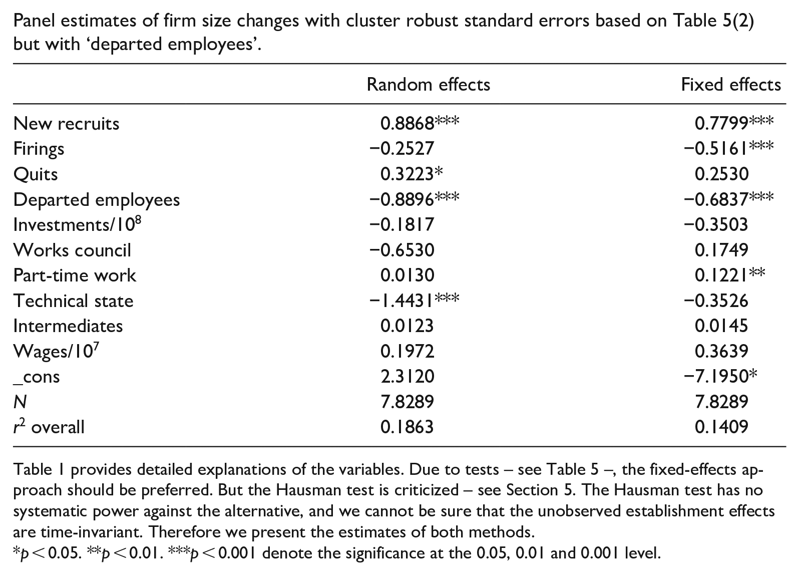
Panel estimates of firm size changes with cluster robust standard errors based on Table 5(2) but with ‘departed employees’.

Random effects Fixed effects

New recruits 0.8868*** 0.7799***

Firings −0.2527 −0.5161***

Quits 0.3223* 0.2530

Departed employees −0.8896*** −0.6837***

Investments/10⁸ −0.1817 −0.3503

Works council −0.6530 0.1749

Part-time work 0.0130 0.1221**

Technical state −1.4431*** −0.3526

Intermediates 0.0123 0.0145

Wages/10⁷ 0.1972 0.3639

_cons 2.3120 −7.1950*

N 7.8289 7.8289

r² overall 0.1863 0.1409

Table 1 provides detailed explanations of the variables. Due to tests – see Table 5 –, the fixed-effects approach should be preferred. But the Hausman test is criticized – see Section 5. The Hausman test has no systematic power against the alternative, and we cannot be sure that the unobserved establishment effects are time-invariant. Therefore we present the estimates of both methods.

*
p < 0.05. **p < 0.01. ***p < 0.001 denote the significance at the 0.05, 0.01 and 0.001 level.

	Random effects	Fixed effects
New recruits	0.8868***	0.7799***
Firings	−0.2527	−0.5161***
Quits	0.3223*	0.2530
Departed employees	−0.8896***	−0.6837***
Investments/10⁸	−0.1817	−0.3503
Works council	−0.6530	0.1749
Part-time work	0.0130	0.1221**
Technical state	−1.4431***	−0.3526
Intermediates	0.0123	0.0145
Wages/10⁷	0.1972	0.3639
_cons	2.3120	−7.1950*
N	7.8289	7.8289
r² overall	0.1863	0.1409

Appendix 4

Sensitivity tests on the difference between coefficients of new recruits of two specifications.

(1) or (2) (2) or (5) (3) or (5) (1) or (5)

(i) or (iv) (ii) or (iii) (ii) or (iv) (iii) or (iv)

A 0.44 22.18*** 0.22 21.79***

B 0.48 11.93*** 0.002 12.29***

1.91* 0.36 1.08 0.56

(1)–(5) are the specifications in Table 4, where in A different and in B the same observations for (1)–(5) are used. (i)–(iv) are based on crisis peak estimates in Tables 7 –9; (i) dot-com; (ii) finance crisis; (iii) corona crisis; (iv) Ukraine war. The presented test statistics are asymptotically standard normal distributed.

*
p < 0.05. **p < 0.01. ***p < 0.001 denote the significance at the 0.05, 0.01 and 0.001 level.

	(1) or (2)	(2) or (5)	(3) or (5)	(1) or (5)
A	0.44	22.18***	0.22	21.79***
B	0.48	11.93***	0.002	12.29***
	1.91*	0.36	1.08	0.56

Appendix 5

Sensitivity tests on the differences between coefficients of quits and firings on firm size of two crises.

Dot-com and finance crisis (2000/2008) Finance and corona crisis (2008/2020) Corona crisis and Ukraine war (2020/2022) Dot-com crisis and Ukraine war (2000/2022)

Quits 1.50 0.92 0.97 1.51

Firings −1.92* −1.74* −1.99* −1.81*

Departed employees −2.21* 1.48 −1.59 −2.34**

Investments/10⁷ −1.73* 2.75** −0.77 1.52

Technical status 1.08 −1.65* −0.11 −0.93

Works council −0.21 −0.58 −0.49 −1.45

Wages/10⁷ −0.68 −0.54 0.63 −0.66

Part-time work −1.63 −0.05 0.58 0.92

Intermediates −0.51 0.43 0.05 0.07

Test statistics are asymptotically standard normal distributed.

*
p < 0.05. **p < 0.01 denote the significance at the 0.05 and 0.01 level.

	Dot-com and finance crisis (2000/2008)	Finance and corona crisis (2008/2020)	Corona crisis and Ukraine war (2020/2022)	Dot-com crisis and Ukraine war (2000/2022)
Quits	1.50	0.92	0.97	1.51
Firings	−1.92*	−1.74*	−1.99*	−1.81*
Departed employees	−2.21*	1.48	−1.59	−2.34**
Investments/10⁷	−1.73*	2.75**	−0.77	1.52
Technical status	1.08	−1.65*	−0.11	−0.93
Works council	−0.21	−0.58	−0.49	−1.45
Wages/10⁷	−0.68	−0.54	0.63	−0.66
Part-time work	−1.63	−0.05	0.58	0.92
Intermediates	−0.51	0.43	0.05	0.07

Funding

The author(s) received no financial support for the research, authorship, and/or publication of this article.

ORCID iD

Lisa Bellmann

References

1.
Abowd JM Corbel P Kramarz F (1999) The entry and exit of workers and the growth of employment: An analysis of French establishments. Review of Economics and Statistics 81(2): 170–187.

2.
Acemoglu D Aghion P Lelarge C , et al. (2007) Technology, information and the decentralization of the firm. Quarterly Journal of Economics 122(4): 1759–1799.

3.
Aksoy CG Barrero JM Bloom N , et al. (2022) Working from home around the world. IZA Discussion Paper No. 15540. Available at: https://www.iza.org/publications/dp/15540/working-from-home-around-the-world (accessed 16 July 2024).

4.
Askenazy P Galbis EM (2007) The impact of technological and organizational changes on labor flows. Evidence on French establishments. Labour 21(2): 265–301.

5.
Bachmann R Bayer C Merkl C , et al. (2021) Worker churn in the cross section and over time: New evidence from Germany. Journal of Monetary Economics 117: 781–797.

6.
Backhaus N (2022) Arbeitszeiten in der Corona-Krise: Länger, Kürzer oder flexibler [Working Tims during the Corona-Crisis: Longer, Shorter or more Flexible]. In: Bellmann L Matiaske W (eds) Ökonomie und Gesellschaft 2022. Jahrbuch 33. Marburg: Metropolis-Verlag, pp.193–226.

7.
Balleer A Gehrke B Lechthaler W , et al. (2016) Does short-time work save jobs? A business cycle analysis. European Economic Review 84: 99–122.

8.
Bazylik S Gibbs M (2022) How is new technology changing job design? IZA World of Labor. Available at: https://wol.iza.org/uploads/articles/621/pdfs/how-is-new-technology-changing-job-design.pdf?v=1 (accessed 16 July 2024).

9.
Bellmann L Bellmann L Hübler O (2024) Labour mobility, short-time work and working from home: Establishments’ behaviour during the COVID-19 crisis. International Journal of Manpower 45(6): 1262–1278.

10.
Bellmann L Gerner HD (2011) Reversed roles? Wage and employment effects of the current crisis. Research in Labour Economics 32(5): 181–206.

11.
Bellmann L Gerner HD Laible MC , et al. (2016) The German labour market puzzle in the great recession. In: Askenazy P Bellmann L Bryson A (eds) Productivity Puzzles Across Europe, Studies of Policy Reform. Oxford: Oxford University Press, pp.187–235.

12.
Belloni A Chen D Chernozhukov V (2012) Sparse models and methods for optimal instruments with an application to eminent domain. Econometrics 80(6): 2369–2429.

13.
Belloni A Chernozhukov V (2013) Least squares after model selection in high-dimensional sparse models. Bernoulli 19(2): 521–547.

14.
Bendel RB Afifi AA (1977) Comparison of stopping rules in forward “stepwise” regression. Journal of the American Statistical Association 72(357): 46–53.

15.
Bloom N Garicano L Sadun R , et al. (2014) The distinct effects of information technology and communication technology on firm organization. Management Science 60(12): 2859–2885.

16.
Boeri T Bruecker H (2011) Short-time work benefits revisited. Some lessons from the great recession. Economic Policy 26(68): 697–765.

17.
Boockmann B Steffes S (2010) Workers, firms, or institutions: What determines job duration for male employees in Germany? Industrial and Labor Relations Review 64(1): 109–127.

18.
Breusch TS Pagan AR (1980) The Lagrange multiplier test and its applications to model specification in econometrics. Review of Economic Studies 47(1): 239–253.

19.
Burda MC Hunt J (2011) What explains the German labor market miracle in the great recession? Brookings Papers on Economic Activity 2011(1): 273–319.

20.
Castro Silva H Lima F (2017) Technology, employment, and skills: A look into job duration. Research Policy 46(8): 1519–1530.

21.
Dauth W Findeisen S Suedekum J , et al. (2021) The adjustment of labor markets to robots. Journal of the European Economic Association 19(6): 3104–3153.

22.
Davis SJ Faberman RJ Haltiwanger J (2006) The flow approach to labor markets: New data sources and micro–macro links. Journal of Economic Perspectives 20(3): 3–26.

23.
Davis SJ Haltiwanger J Schuh S (1996) Job Creation and Destruction. Cambridge: MIT Press.

24.
Di Cintio M Grassi E (2022) Labour flows and R&D: A quantile regression analysis. International Journal of Business and Social Science 13(1): 2219–1933.

25.
Dietz M Stops M Walwei U (2010) Safeguarding jobs through labour hoarding in Germany. Applied Economic Quarterly Supplement 61(1): 125–149.

26.
Dustmann C Fitzenberger B Schönberg U , et al. (2014) From sick man of Europe to economic superstar: Germany’s resurgent economy. Journal of Economic Perspectives 28(1): 167–188.

27.
Efron B Hastie T Johnstone I , et al. (2004) Least angle regression. Annals of Statistics 32(2): 407–451.

28.
Ellguth P Kohaut S (2009) Tarifbindung und betriebliche Interessenvertretung in Ost und West. Schwund unter sicherem Dach. IAB-Forum 2: 68–75.

29.
Fackler D Schnabel C Stegmaier J (2021) Personnel adjustment during the COVID-19 pandemic: Did co-determination make a difference? IZA Discussion Paper No. 14873. Available at: https://www.iza.org/publications/dp/14873/personnel-adjustments-during-the-covid-19-pandemic-did-co-determination-make-a-difference (accessed 16 July 2024).

30.
Fahr R Sunde U (2009) Did the Hartz reforms speed-up the matching process? A macro-evaluation using empirical matching functions. German Economic Review 10(3): 284–316.

31.
Fentanes O Gathen J (2022) Growth and the firm-size distribution over the long-run. Unpublished paper. Available at: https://steg.cepr.org/sites/default/files/2022-01/Speed%208C%20Paper%20Gathen.pdf (accessed 16 July 2024).

32.
Gomez P (2010) Labour market flow. Facts from the United Kingdom. IZA Discussion Paper No. 5327. Available at: https://www.iza.org/publications/dp/5327/labour-market-flows-facts-from-the-united-kingdom (accessed 16 July 2024).

33.
Greene WH (ed.) (1997) Econometric Analysis, 3rd edn. Upper Saddle River, NJ: Prentice Hall.

34.
Haltiwanger JC Hyatt HR Kahn LB , et al. (2018) Cyclical job ladders by firm size and firm wage. American Economic Journal Macroeconomics 10(2): 52–85.

35.
Hausman JA (1978) Specification tests in econometrics. Econometrics 46(6): 1251–1271.

36.
Hershbein B Kahn LB (2018) Do recessions accelerate routine-biased technological change? Evidence from vacancy postings. American Economic Review 108(7): 1737–1772.

37.
Heß P Janssen S Leber U (2023) The effect of automation technology on workers’ training participation. Economics of Education Review 96(C): 102438.

38.
Hübler O (1989) Ökonometrie [Econometrics]. Stuttgart, New York: UTB Gustav Fischer Verlag.

39.
Hyatt H McEntarfer E (2012) Job-to-job flows in the great recession. American Economic Review 102(3): 580–583.

40.
Kölling A (2000) The IAB-establishment panel. Schmollers Jahrbuch 120(2): 291–300.

41.
Kumar KP Rajan RG Zingales L (1999) What determines firm size? NBER Working Paper 7208. Available at: https://www.nber.org/system/files/working_papers/w7208/w7208.pdf (accessed 16 July 2024).

42.
Launov A Wälde K (2014) Folgen der Hartz-Reformen für die Beschäftigung [Emloyment Effects of Hartz Reforms]. Wirtschaftsdienst 94(2): 112–117.

43.
Lazear EP Spletzer JR (2012) Hiring, churn, and the business cycle. American Economic Review 102(3): 575–579.

44.
Leeb H Pötscher BM (2008) Can one estimate the unconditional distribution of post-model-selection estimators? Economic Theory 24(02): 338–376.

45.
Lin K-H Aragao C Dominguez G (2021) Firm size and employment during the pandemic. Sociological Research for a Dynamic World 7: 1–16.

46.
Möller J (2010) The German labor market response in the world recession – De-mystifying a miracle. Journal for Labour Market Research 42(4): 325–336.

47.
Moscarini G Postel-Vinary F (2009) The timing of labor market expansions: New facts and new hypothesis. In: Acemoglu D Rogoff K Woodford M (eds) NBER Macroeconomics Annual 2008, vol. 23. Chicago, IL: University of Chicago Press, pp.1–51.

48.
Moscarini G Postel-Vinay F (2012) The contribution of large and small employers to job creation in times of high and low unemployment. American Economic Review 102(6): 2509–2539.

49.
Poschke M (2018) The firm size distribution across countries and skill-biased change in entrepreneurial technology. American Economic Journal Macroeconomics 10(3): 1–41.

50.
Schumpeter JA (1934) The Theory of Economic Development: An Inquiry Into Profits, Credit, Interest, and the Business Cycle. New Brunswick and London: Harvard Economic Studies.

51.
Song Y (2009) Training, technological changes, and displacement. Journal of Labor Research 30(3): 201–218.

52.
Spermann A (2012) The new role of temporary agency work in Germany. In: Bouncken RB Bellmann L Bornewasser M (eds) Die neue Rolle der Zeitarbeit in Deutschland. Beiträge zur Flexibilisierung, vol. 3. Hampp: München und Mering, pp.203–224.

53.
Tibshirani R (1996) Regression shrinkage and selection via the Lasso. Journal of the Royal Statistical Society Series A (General) 58(1): 267–288.

54.
Zapf I Brehmer W (2010) Flexibility during the Crisis: Working Time Accounts Have Proven their Worth. IAB-Kurzbericht 22(2/2016): 1–8.