
Abstract
Background:
Modified Rankin Scale (mRS) scores are used to measure functional outcomes after stroke. Researchers create horizontal stacked bar graphs (nicknamed “Grotta bars”) to illustrate distributional differences in scores between groups. In well-conducted randomized controlled trials, Grotta bars have a causal interpretation. However, the common practice of exclusively presenting unadjusted Grotta bars in observational studies can be misleading in the presence of confounding. We demonstrated this problem and a possible solution using an empirical comparison of 3-month mRS scores among stroke/TIA patients discharged home versus elsewhere after hospitalization.
Patients and methods:
Using data from the Berlin-based B-SPATIAL registry, we estimated the probability of being discharged home conditional on prespecified measured confounding factors and generated stabilized inverse probability of treatment (IPT) weights for each patient. We visualized mRS distributions by group with Grotta bars for the IPT-weighted population in which measured confounding was removed. We then used ordinal logistic regression to quantify unadjusted and adjusted associations between being discharged home and the 3-month mRS score.
Results:
Of 3184 eligible patients, 2537 (79.7%) were discharged home. In the unadjusted analyses, those discharged home had considerably lower mRS compared with patients discharged elsewhere (common odds ratio, cOR = 0.13, 95% CI: 0.11–0.15). After removing measured confounding, we obtained substantially different mRS distributions, visually apparent in the adjusted Grotta bars. No statistically significant association was found after confounding adjustment (cOR = 0.82, 95% CI: 0.60–1.12).
Discussion and conclusion:
The practice of presenting only unadjusted stacked bar graphs for mRS scores together with adjusted effect estimates in observational studies can be misleading. IPT weighting can be implemented to create Grotta bars that account for measured confounding, which are more consistent with the presentation of adjusted results in observational studies.
Introduction
Measures of functional outcome after stroke are important outcomes of interest when aiming to estimate the effect of an intervention or other exposure of interest in patients with stroke. The most commonly used functional outcome measure in stroke research is the ordinal modified Rankin Scale (mRS).1 –3
James C. Grotta 4 popularized the use of horizontal stacked proportional bar graphs, nicknamed “Grotta bars,” to create clear, visual representations of mRS distributions by exposure/treatment status. Grotta bars display the proportion of individuals having a certain mRS category on the x-axis, stratified by exposure group (y-axis), and generally include lines connecting the segment boundaries of each mRS category.4,5 Following their appearance in the 1996 National Institute of Neurological Disorders and Stroke Tissue Plasminogen Activator randomized control trial (RCT),4,6 Grotta bars became the conventional method to visualize mRS results in stroke RCTs. 5
In observational studies, however, readers may be tempted to endow these simple comparisons of outcome distributions with a causal interpretation, even though they do not account for confounding. Nevertheless, it is common practice to present Grotta bars to visualize the observed mRS distribution among exposed and unexposed individuals, but then rely on statistical models to generate a confounding-adjusted estimate of the effect of the exposure of interest on the outcome.7 –11 This approach can lead to a mismatch between the unadjusted exposure-outcome association reflected in the stacked bar graph visualization and the reported adjusted effect estimate.11,12
Some methods have been employed in the literature in an effort to account for confounding in these visualizations, such as stratified Grotta bars13,14 and Grotta bars produced from a propensity score-matched subset of the larger cohort.15 –17 However, these methods only allow for the presentation of the mRS distribution in specific subgroups and do not visualize the marginal mRS distribution (the one typically reported in RCTs). 18 The emphasis on modern causal inference methods and target trial emulation in epidemiology, 18 has led some authors to use inverse probability of treatment (IPT) weighting to produce Grotta bars adjusted for confounding.19,20
In this study, we present an application of IPT weighting to create stacked bar graphs that account for measured confounding in observational settings using an intuitive clinical example and data from a large stroke registry in Berlin, Germany.
Patients and methods
Inverse probability of treatment weighting: Approach and rationale
In observational studies, control of confounding (i.e. adjustment for common causes of the exposure and outcome) is essential to obtain correct causal estimates for the effect of an exposure on an outcome. 18 In this article, we focus on IPT weighting, a technique that generates a weight for each individual in the study that is inversely proportional to that individual’s probability of receiving the exposure (e.g. treatment) they actually received. 21 By applying these weights to the study population, a re-weighted study population termed “pseudo-population,” is created.18,21 In this pseudo-population, measured confounding is removed, since the weighting mechanism creates an artificial independence between the measured participant characteristics (i.e. the measured confounding variables) and the exposure status. Under the causal inference assumptions of conditional exchangeability (no unmeasured confounding), consistency, positivity, no measurement error, and no model misspecification, the computed association between the exposure and the outcome in the pseudo-population is an unbiased estimate of the true causal effect.18,21
Under these assumptions, the pseudo-population obtained by IPT weighting is equivalent to an RCT. 18 Furthermore, the proportion of exposed (or unexposed) individuals in a given mRS category in the pseudo-population represents an unbiased estimate of the probability of being in that mRS category in a counterfactual world in which everyone is exposed (or unexposed).18,22 The pseudo-population created by IPT weighting can then be used to generate Grotta bars in the usual way, which will conveniently contain built-in confounding adjustment.
Clinical question
To illustrate the issue of confounding and its impact on (unadjusted) Grotta bars, we chose a clinical question for which confounding is an obvious concern. We aimed to estimate the effect, among TIA and stroke patients living at home before the index event, of being discharged home from the hospital on the mRS of the patients 3 months after hospital admission. We expect that in the visualization of the Grotta bars using observed data, the proportion of patients in lower mRS categories (indicating better outcomes) will be much higher among individuals discharged home compared with individuals not discharged home. This is because individuals are more likely to be discharged home if they have characteristics that will lead to a better functional outcome at 3 months. Certainly, the unadjusted association between exposure and outcome cannot be interpreted as causal since it is strongly confounded, for example, by age, other medical conditions, stroke severity, and functional status at discharge.
Data source
To answer this causal question, we used data from the “Berlin – specific acute therapy in ischemic or hemorrhagic stroke with long-term follow-up” (B-SPATIAL) registry (Clinicaltrials.gov identifier: NCT03027453), which received approval for scientific evaluation by the ethics committee of Charité - Universitätsmedizin Berlin (EA1/208/21). Patients were informed about their participation in the B-SPATIAL registry with an opt-out mechanism. 23 Details about the registry can be found in Box 1.
Details about the Berlin – specific acute therapy in ischemic or hemorrhagic stroke with long-term follow-up (B-SPATIAL) registry.
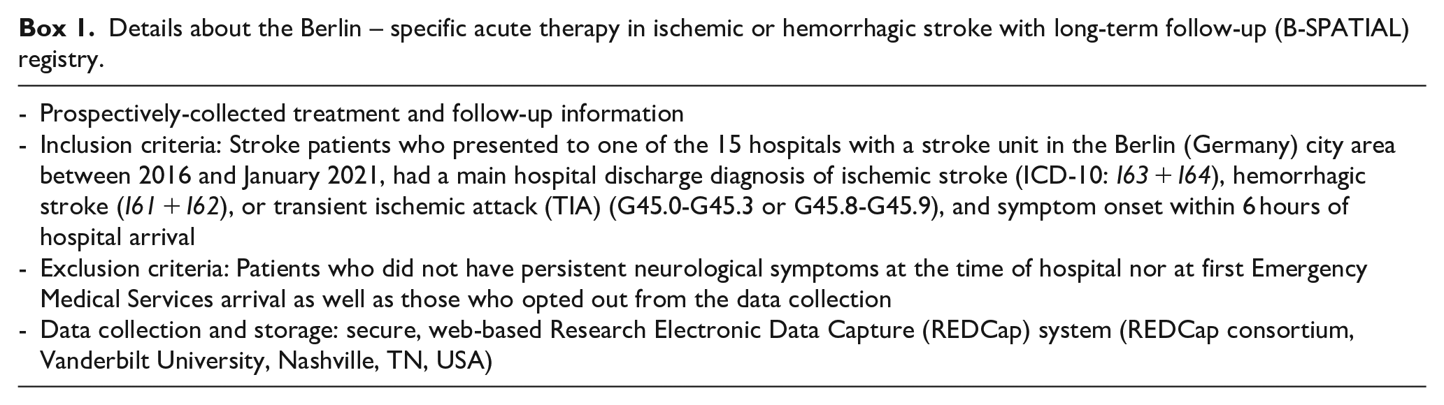
We used data from patients with a diagnosis of TIA, ischemic stroke, or hemorrhagic stroke who were hospitalized in 1 of the 15 hospitals after the index event (we did not consider patients transferred from other hospitals) and who were living at home (i.e. not in a nursing care facility) before the index event. For simplicity, we did not include patients recruited in the B_PROUD interventional study. 10 Furthermore, to be considered eligible for this study population, patients must have been discharged within 1 week of hospital admission, be alive at the time of discharge, and have information about discharge status. To avoid overcomplicating the empirical example with imputation, we performed a complete-case analysis, thus excluding participants with missing values for the outcome (mRS) or any of the considered confounding variables.
Exposure
The exposure of interest was the hospital discharge status after the index stroke or TIA event. The exposure was a binary variable indicating whether the patient was discharged home. The “unexposed” category included being discharged to a rehabilitation facility, nursing care facility, hospice care, another department within the same hospital, or another hospital, as well as having elected to leave the hospital against medical advice.
Outcome
The outcome was the functional disability 3 months after hospital admission, as measured by the ordinal mRS.2,3 The seven possible mRS scores are: 0 (no symptoms), 1 (no significant disability), 2 (slight disability), 3 (moderate disability), 4 (moderately severe disability), 5 (severe disability), and 6 (death).1 –3,5 Information needed to ascertain mRS scores was obtained from an interview with an experienced study nurse or, when patients preferred, via self-reported information obtained by a questionnaire mailed to the patients. Vital status information obtained during follow-up was supplemented with information from the city’s registration office.
Confounding control
To identify the effect of being discharged home on 3-month mRS, we considered the following confounding variables: age, sex (female/non-female), presence of a disease with a life expectancy of less than 1 year (yes/no), TIA diagnosis (yes/no), mRS at hospital admission (numeric), National Institutes of Health Stroke Scale (NIHSS) score at hospital admission (numeric), number of days in hospital before discharge (numeric), and mRS scores at discharge (numeric).
Statistical analyses
We reported frequencies for categorical variables and mean, standard deviation, median, and interquartile ranges for continuous variables stratified by exposure status.
We first created the Grotta bars for the observed data, without adjustment, using the grottaBar R package. 24 Next, we created the Grotta bars using stabilized IPT weights to adjust for confounding as follows: First, we fit a logistic regression with the exposure as the dependent variable and no independent variables (intercept-only model). Second, we fit a logistic regression with the exposure as the dependent variable and the confounding variables as independent variables. Next, we predicted the probability of being exposed (e.g. discharged home) for each individual in the dataset given their values for the confounding variables. Finally, we computed stabilized weights for each individual as the ratio between the probability of being exposed if a person was exposed (or one minus the probability of being exposed if a person was not exposed) as predicted by the intercept-only logistic regression model, divided by the probability of being exposed (or one minus the probability of being exposed) as predicted by the logistic regression with the confounding variables as independent variables.
The individuals from the original population were then copied a number of times equal to their stabilized weights, and all these copies of individuals from the original population comprised the pseudo-population. The use of stabilized weights aims at creating a pseudo-population having the same size as the original study population and with the same proportion of exposed individuals, while leaving no remaining associations between the confounding variables and the exposure. 18 Therefore, by summing the weights for all exposed (or unexposed) individuals within each stratum of the mRS, we obtained the absolute number of individuals within each mRS category in the pseudo-population by exposure status. These absolute numbers of individuals were then used to produce the adjusted Grotta bars.
In some situations, the estimated weights for some individuals can be extreme (e.g. if the estimated probability of being discharged home was very low, but the individual was actually discharged home), and this is known to reduce precision.21,25 A common practice in this scenario is to truncate extreme weights, finding an acceptable trade-off between bias and variance. 21 We truncated the weights at the 0.7th and 99.3th percentiles to obtain well-behaved weights. 21
To quantify the unadjusted association between being discharged home and the 3-month mRS, we fit an ordinal logistic regression with mRS as the dependent variable and the discharge status as the independent variable. The association adjusted for measured confounding was quantified by fitting the same model in the aforementioned pseudo-population. For both models, the proportional odds assumption was graphically assessed. 26 The 95% confidence interval (CI) for the adjusted common odds ratio (cOR) was obtained by repeating the analysis (with the same truncation of weights) over 500 bootstrapped datasets, using the 2.5% and 97.5% percentiles of the ordinal logistic regression coefficient estimates as the lower and upper limits.
All analyses were conducted using R version 4.0.3 and RStudio 2021.09.1.
Results
From the total B-SPATIAL registry (16,126 records), 4167 patients with stroke/TIA met the eligibility criteria for this study (Figure 1). After we further excluded 983 patients with missing values, 3184 patients remained for our analyses.
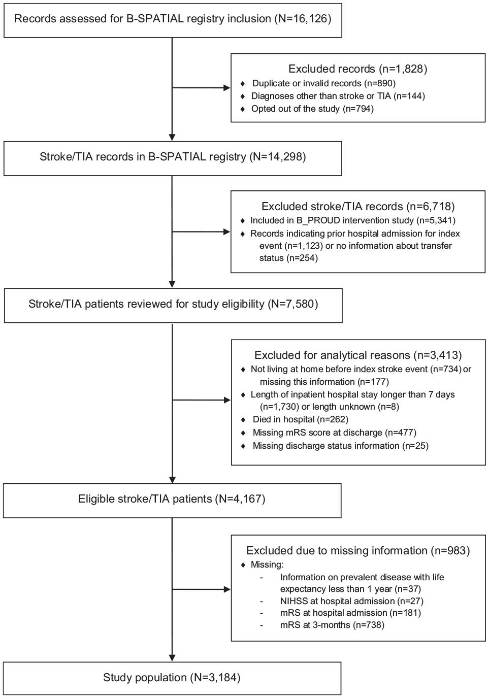
Flow diagram for study population.
Of the 3184 patients, 2537 (79.7%) were discharged home from the hospital and 647 (20.3%) were not. As expected, in the original study population, patients who were discharged home were on average younger, had fewer severe diseases with a life expectancy of less than 1 year, more frequently had a diagnosis of TIA, had a lower stroke severity and better functional outcomes at hospital admission, and had better functional outcomes at discharge (Table 1).
Characteristics of individuals in the original study population (B-SPATIAL registry) and in the pseudo-population obtained using inverse probability of treatment weighting with (truncated) stabilized weights.
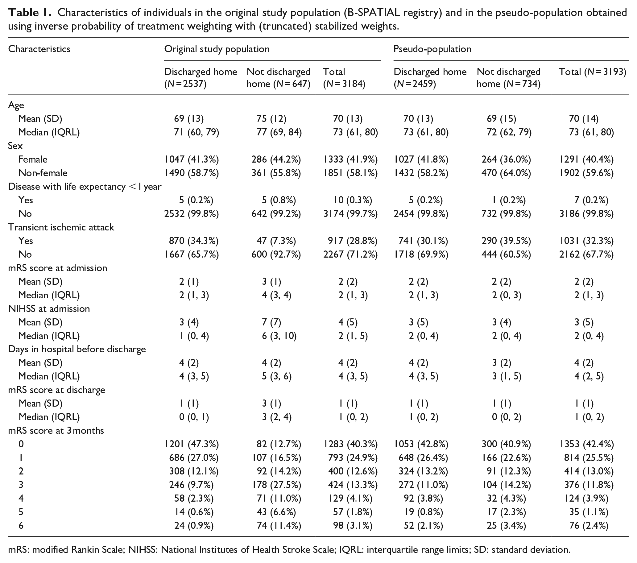
mRS: modified Rankin Scale; NIHSS: National Institutes of Health Stroke Scale; IQRL: interquartile range limits; SD: standard deviation.
The unadjusted Grotta bars display a striking difference in the distributions of 3-month mRS scores between the group of patients who were discharged home and the group who were not (Figure 2, top panel). We found a strong, statistically significant association between being discharged home and 3-month mRS (cOR = 0.13, 95% CI: 0.11–0.15). Indeed, patients who were actually discharged home had comparatively lower mRS scores at 3 months; for example, 74.4% of patients discharged home had an mRS score of 0 or 1 compared with only 29.2% of patients not discharged home (Table 1). Furthermore, 11.4% of patients who were not discharged home died within 3 months of hospital admission compared with only 0.9% of patients discharged home (Table 1).
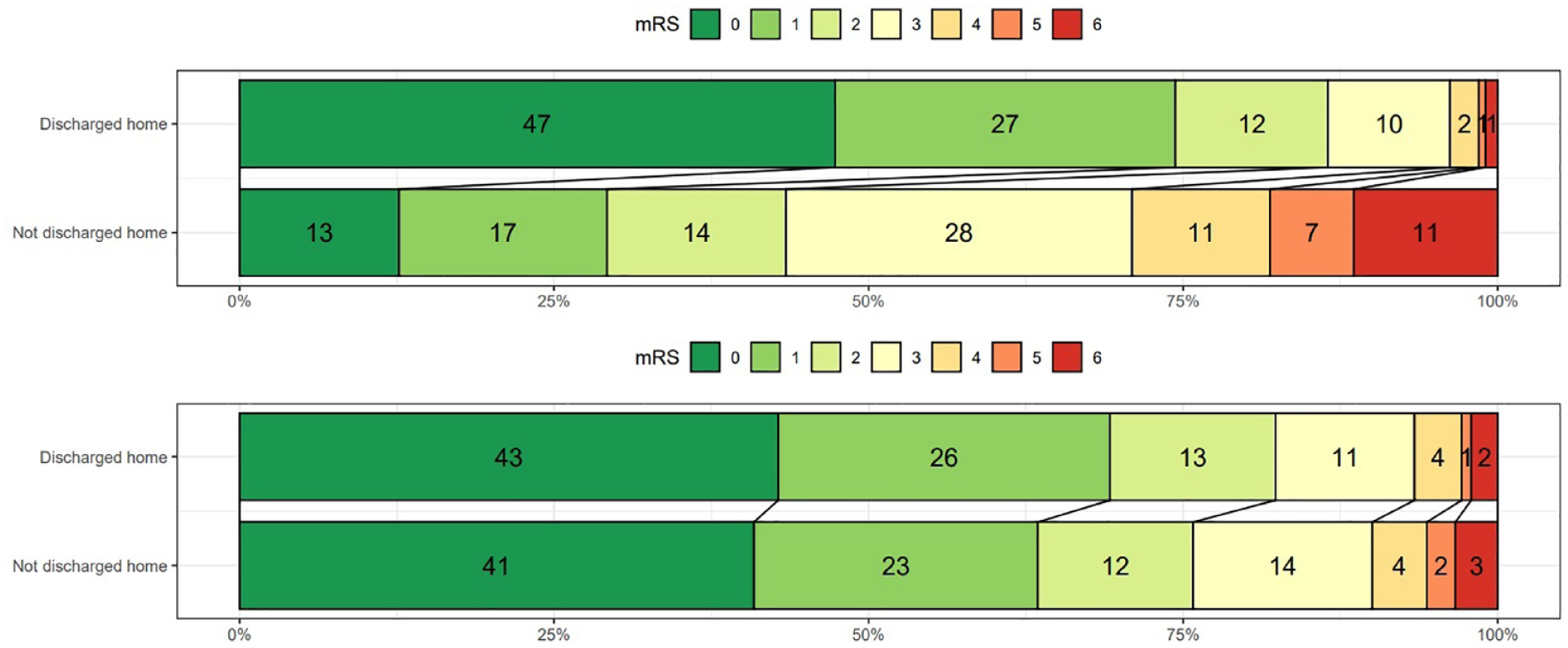
Distribution of modified Rankin Scale (mRS) scores at 3-month after hospital admission among patients with transient ischemic attack or stroke in B-SPATIAL registry stratified according to discharge status in the original study population (top) and in the pseudo-population generated after applying inverse probability of treatment weighting (bottom).
The IPT weighting resulted in substantial balancing of the confounding variables; in the IPT-weighted pseudo-population, the distribution of the confounding variables in the exposed group was very similar to the distribution in the unexposed group (Table 1).
The adjusted Grotta bars created using data from the IPT-weighted pseudo-population (Figure 2, bottom panel) reflect very different mRS distributions for both groups compared with the unadjusted stacked bars. The unadjusted Grotta bars show a strong, highly confounded association. This is expected, since individuals who are discharged home have values for the confounding variables that, in turn, are associated with better functional outcome at 3 months.
On the other hand, the adjusted Grotta bars reflect outcome proportions per group that are more consistent with a causal interpretation because the associations between the measured confounding variables and the discharge status were removed in the weighted pseudo-population. In this way, the IPT weighting removed a large part of the originally observed difference in the mRS distributions between the exposure groups attributable to this confounding. In the pseudo-population, the proportion of patients discharged to home in mRS score categories 0 or 1 decreased to 69.2%, whereas it increased to 63.5% in patients not discharged home (Figure 2). Also, the proportion of stroke patients discharged home who died within 3 months increased to 2.1%, while it decreased to 3.4% for patients not discharged to home. We found no statistically significant association between the exposure and the outcome after adjustment for measured confounding (cOR = 0.82, 95% CI: 0.60–1.12).
Discussion
In this study, we showed to what extent unadjusted and adjusted horizontal stacked bar graphs (“Grotta bars”) differ for an applied clinical example in observational stroke research. Upon comparing stroke and TIA patients discharged home with patients not discharged home, those discharged home had a tremendously more favorable distribution of mRS scores according to the unadjusted Grotta bars. Using an IPT-weighted pseudo-population, we created adjusted Grotta bars to remove confounding. The adjusted Grotta bars showed a substantially different distribution of mRS scores in the two groups, indicating that discharge home was far less beneficial for functional outcome than the unadjusted bars would have led us to believe. Our results highlight that, in observational studies, unadjusted Grotta bars cannot generally be endowed with a causal interpretation because they merely represent an association partially or even fully explainable by confounding.
Discharge status is strongly associated with 3-month functional outcome status after stroke. 27 We chose this example as the potential for strong confounding is obvious, and information about the main, important confounding variables was available. Clinical intuition should caution us against endowing the unadjusted Grotta bars with a causal interpretation in this scenario, since specific characteristics and/or clinical parameters that lead to the decision to discharge patients home are also associated with a better prognosis.
After adjustment, we found no evidence of an association between being discharged home and 3-month functional outcome. Of course, the hypothetical “target” randomized controlled trial we emulated 28 in this study would not be reasonable in the real world due to ethical concerns. However, RCTs in Canada 29 and in Australia 30 investigating a slightly different causal questions (e.g. the effect of being discharged home with early supported discharge services vs. usual in-hospital care) in other settings also found no differences in patients’ long-term functional outcomes. Importantly, the eligibility criteria of these RCTs restricted enrollment to those individuals who were rather independent and had favorable conditions at home to promote recovery.29 –31 On the other hand, an individual patient meta-analysis comparing hospitalized patients randomized to any type of at-home “early supported discharge” with those who received conventional care found a lower risk of death or dependency among those discharged home. 32
We primarily chose this clinical application example for illustrative and didactic purposes; a sharp change in the mRS distribution is observed after confounding adjustment, resulting in a completely different interpretation of the results for the unadjusted versus adjusted Grotta bars. Grotta bars have several advantages in that they deliver important information in an accessible, intuitive way. These stacked proportional bar graphs accentuate observed differences between exposed and unexposed individuals across the entire mRS distribution, rather than trying to summarize this shift with a single effect estimate alone (e.g. a common odds ratio from ordinal logistic regression) or through dichotomization of the mRS scores, which results in a loss of information.33,34
Given these advantages, it is no surprise that Grotta bars are nearly ubiquitous in stroke RCTs. It also explains their presence in the observational stroke literature, albeit mostly in an unadjusted form, with a few exceptions,15 –17,19,20 despite the mismatch between the information they convey and the reported adjusted estimates of the primary effects of interest. As illustrated by our clinical application, adjusted Grotta bars obtained by IPT weighting can be endowed with a causal interpretation if a suitable design and analytical approach are properly implemented and causal inference assumptions hold. 18 By using this method, the advantages of using Grotta bars can be extended from RCTs to observational research.
The use of modern causal inference methods, 18 such as IPT weighting, is becoming increasingly common.7 –9,19,20,35 –38 In addition to adjusting for measured sources of confounding, IPT weighting-based approaches have advantages as they estimate the marginal causal effect in the full study population (incorporating effect heterogeneity across subgroups). The applicability of these methods is not only restricted to observational cohort studies, but they can also be useful in non-randomized interventional studies. 39 Moreover, IPT weighting can accommodate complex, time-varying exposures and confounding structures in studies with repeated measurements and differential censoring of study participants during follow-up.18,21 Annotated analytic code to apply IPT weighting across a diverse range of software (e.g. SAS, Stata, and R) is openly available online. 40
Though IPT weighting lends itself particularly well to the creation of adjusted Grotta bars, we identified other approaches that also attempted to provide a more coherent visual representation to accompany adjusted point estimates in observational studies (i.e. through stratification by relevant variables13,14 or restriction to the propensity score-matched subset of the original study population15 –17). These Grotta Bar adaptations account for confounding by reporting the mRS distributions restricted to specific subgroups of the study population (i.e. by strata of a confounder, or only among matched individuals). However, the mRS distribution visualized in this way is different from the one that would have been observed had an equivalent RCT been conducted, since RCTs target the marginal mRS distribution for the entire study population. 18
Stroke researchers may be less familiar with the statistical methods needed to build adjusted Grotta bars, which involve some extra steps compared with traditional approaches. To overcome this potential complexity and to support researchers interested in creating their own adjusted Grotta bars, we present a roadmap inspired by our clinical example (Figure 3). In the roadmap, we illustrate step by step how to implement IPT weighting with stabilized weights to build adjusted Grotta bars for research questions about the effect of a binary exposure measured at a single time point on mRS. The method requires the assumptions of conditional exchangeability (no unmeasured confounding), positivity, consistency, no measurement error, and no model misspecification. 18 The extent to which these assumptions are actually satisfied in a given observational study depends on the specific application and its circumstances. If these assumptions hold, then the adjusted Grotta bars can be interpreted as showing the outcome distributions (among exposed and unexposed) that would have been observed in an equivalent RCT.
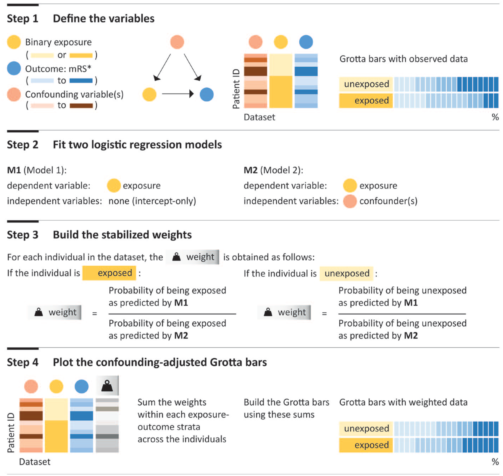
Road map to build adjusted Grotta bars inspired by our clinical application. This step-by-step protocol relies on inverse probability of treatment weighting with stabilized weights (without truncation) for a research question about effect of a binary exposure measured at a single time point (in two shades of yellow) on the outcome, modified Rankin Scale (mRS; in four shades of blue, representing four levels). In this simple scenario, the confounding variable has four levels (light to dark red) with higher levels leading the individual to be less likely to receive the exposure and more likely to have a worse outcome. The stabilized weights are depicted in gray, with darker colors indicating larger weights. We assumed conditional exchangeability, positivity, consistency, no measurement error, and no model misspecification, as is customary in causal inference research. In some applications, truncation during step 3 may be deemed appropriate (for further reading on this topic, see Cole and Hernán 21 ). *For simplicity and didactic purposes, we depicted mRS as a variable with four levels (with darker colors indicating worse outcomes) instead of seven levels.
Strengths and limitations
Strengths of our study include the use of rigorously collected data according to standardized protocols from a metropolitan stroke registry with complete coverage of all the city’s stroke units, the availability of many covariates needed to address major, known sources of confounding, and the use of a modern causal inference method to adjust for confounding.
Some limitations should be considered when interpreting our results. First, the IPT weighting technique we implemented to generate adjusted distributions of the mRS scores can only remove measured sources of confounding. A systematic review seeking to identify factors associated with discharge destination identified many of the variables included in our confounding adjustment strategy. 41 Though unlikely to contribute a large amount of residual confounding, some variables typically not measured in registries, such as cognitive ability, cohabitation, and/or mental health status, may have contributed to the discharge decision. For this reason, we cannot rule out some unmeasured confounding as an explanation for our findings.
Second, we performed complete case analysis, excluding participants with missing information for any of the included covariates, which may have introduced selection bias. In the trade-off between adding substantial complexity by implementing imputation procedures and keeping things simple, for didactic purposes, we opted for a complete case analysis to not distract from our focus on confounding adjustment. However, we emphasize that if a complete case analysis is not deemed appropriate, this adjustment method can also be applied along with imputation techniques. In a recent real-world application, after conducting multiple imputation by chained equations, adjusted Grotta bars were presented separately for each imputed dataset. 39
Third, we cannot exclude that despite the standardized data collection in the B-SPATIAL registry some information was misclassified. Furthermore, for simplicity, in our operationalization of discharge status, we did not consider a minimum hospitalization time threshold. Therefore, patients transferred to another hospital for future acute stroke work up or treatment were classified as unexposed (not discharged home). However, after excluding patients (n = 83) who were discharged within 24 h of hospital admission, we did not observe a meaningful difference in our results.
Finally, we did not incorporate aspects related to statistical inference (i.e. through the quantification of uncertainty), as traditional Grotta bars do not incorporate this information (neither in RCTs nor observational studies). However, we point readers to an intuitive proposal to graphically incorporate information about variability. 5 This method could deliver more transparent representation of variability, especially in cases of smaller sample sizes, in conjunction with the IPT-weighted Grotta bars, but this goes beyond the scope of the present study.
Conclusion
Using an empirical example, we illustrate how IPT weighting can be used to create Grotta bars adjusted for measured sources of confounding in observational settings. While presenting unadjusted Grotta bars in observational studies for descriptive purposes is useful, we encourage stroke researchers aiming to answer a causal question to additionally present adjusted Grotta bars together with their adjusted effect estimates for consistency in presentation of their results.
Footnotes
Acknowledgements
We thank the Berlin Data Protection Office (Berliner Beauftragte für Datenschutz und Informationsfreiheit) and the data protection officer of the Charité–Universitätsmedizin Berlin for advice and support. We are grateful to all collaborating hospitals and the study nurses for their continued engagement.
Declaration of conflicting interests
The author(s) declared the following potential conflicts of interest with respect to the research, authorship, and/or publication of this article: JLR reports having received a grant from Novartis Pharma for conducting a self-initiated research project outside this work. RHG reports receiving funds from the German Academic Exchange Service (DAAD). HJA reports receiving institutional grants from the Gemeinsamer Bundesausschuss (G-BA – German Federal Joint Committee) outside the submitted work, and receiving personal fees from AstraZeneca, Bayer Vital, Boehringer Ingelheim, Bristol Myers Squibb, Novo Nordisk, Pfizer, Roche and Sanofi. TK reports outside the submitted work having received research grants from the Gemeinsamer Bundesausschuss (G-BA – German Federal Joint Committee), the Bundesministerium für Gesundheit (BMG – German Federal Ministry of Health). He further has received personal compensation from Eli Lilly & Company, Teva Pharmaceuticals, TotalEnergies S.E., the BMJ, and Frontiers. MP reports outside the submitted work having received partial funding for a self-initiated research project from Novartis Pharma and being awarded a research grant from the Center for Stroke Research Berlin (private donations).
Funding
The author(s) disclosed receipt of the following financial support for the research, authorship, and/or publication of this article: The B-SPATIAL registry was funded by the German Federal Ministry of Education and Research (BMBF) and the German Research Foundation (DFG), granted to the Center for Stroke Research Berlin. The funders had no role in the design and conduct of the study; collection, management, analysis, and interpretation of the data; preparation, review, or approval of the manuscript; nor decision to submit the manuscript for publication.
Informed consent
The “Berlin – specific acute therapy in ischemic or hemorrhagic stroke with long-term follow-up” (B-SPATIAL) registry used an opt-out mechanism for patient inclusion (See ref 23). After their index event, patients were informed in writing about the inclusion of their record in the B-SPATIAL registry and had multiple options to opt out.
Ethical approval
The scientific evaluation of B-SPATIAL registry data (Clinicaltrials.gov identifier: NCT03027453) was approved by the ethics committee of Charité - Universitätsmedizin Berlin (EA1/208/21).
Guarantors
JLR and MP.
Author contributions
JL Rohmann and M Piccininni conceived the study, and M Piccininni and T Kurth designed the clinical application. HJ Audebert provided clinical insights. R Huerta-Gutierrez performed a literature review and summarized its results. JL Rohmann, T Kurth, and M Piccininni planned the statistical analyses, for which M Piccininni wrote the statistical code. All authors contributed to the interpretation of the results. HJ Audebert initiated the B-SPATIAL registry and obtained funding. JL Rohmann and HJ Audebert contributed to registry administration, and provided resources and logistical support. JL Rohmann, T Kurth, and M Piccininni jointly wrote the first draft of the article, which was critically revised by all authors.