Sage Journals: Discover world-class research

Abstract

Background: Propensity score (PS) methods are frequently used within economic evaluations based on nonrandomized data to adjust for measured confounders, but many researchers omit the fact that they cannot adjust for unmeasured confounders. Objective: To illustrate how confounding due to unmeasured confounders can bias an economic evaluation despite PS matching. Methods: We used data from a previously published nonrandomized study to select a prematched population consisting of 121 patients (46.5%) who received endovascular aneurysm repair (EVAR) and 139 patients (53.5%) who received open surgical repair (OSR), in which sufficient data regarding eight measured confounders were available. One-to-one PS matching was used within this population to select two PS-matched subpopulations. The Matched PS-Smoking Excluded Subpopulation was selected by matching patients using a PS model that omitted patients’ smoking status (one of the measured confounders), whereas the Matched PS-Smoking Included Subpopulation was selected by matching patients using a PS model that included all eight measured confounders. Incremental cost-effectiveness ratios (ICERs) were assessed within both subpopulations. Results: Both subpopulations were composed of two different sets of 164 patients. Balance within the Matched PS-Smoking Excluded Subpopulation was achieved on all confounders except for patients’ smoking status, whereas balance within the Matched PS-Smoking Included Subpopulation was achieved on all confounders. Results indicated that the ICER of EVAR over OSR differed between both subpopulations; the ICER was estimated at $157,909 per life-year gained (LYG) within the Matched PS-Smoking Excluded Subpopulation, while it was estimated at $235,074 per LYG within the Matched PS-Smoking Included Subpopulation. Discussion: Although effective in controlling for measured confounding, PS matching may not adjust for unmeasured confounders that may bias the results of an economic evaluation based on nonrandomized data.

Keywords

economic evaluation observational studies propensity scores confounding unmeasured confounder

Randomized controlled trials (RCTs) are generally regarded as the gold standard for determining the relative efficacy of two or more treatments. Furthermore, in cases where costing data are available, they can also be used to conduct economic evaluations comparing the different interventions. Despite their relative strengths, RCTs may lack external validity and, in certain cases, may not be feasible to conduct.¹ Unlike RCTs, studies based on nonrandomized data (e.g., administrative databases, hospital registries) may have stronger external validity, especially when they follow the complete eligible patient population and do not impose specific treatment plans, but are prone to bias, mostly confounding bias (i.e., bias due to the presence of imbalance in confounder distribution among the two exposure groups).² Although the importance of RCTs in clinical sciences is undeniable, it is clear that clinicians and decision makers are recognizing the complementary value of prospective nonrandomized studies.¹ Such a trend is now also starting to be observed within the context of economic evaluations.³ As the use of nonrandomized studies has been increasing, methodological techniques have been proposed to address the issue of confounding bias.⁴

Propensity score (PS) methods are among the most widely used techniques to adjust for confounding bias within comparative effectiveness studies, a trend that also seems to appear within economic evaluations using nonrandomized data.⁵ Briefly, a PS represents the conditional probability of an individual within a specific cohort to receive an exposure over another given a set of specified measured covariates.⁶ PS adjustment is usually conducted through the use of stratification, matching, weighting, or regression analyses.⁷ Although all of these approaches can and have been used to adjust for confounding,⁸ PS matching is generally favored, and multiple studies have found it superior to the other PS methods with regard to its ability to remove the observed imbalance between the two exposure groups.^9–12

However, like many methodological techniques aimed at controlling for confounding bias (e.g., multivariate regressions, covariate matching),^13,14 PS are limited by the fact that they cannot adjust for unmeasured confounding (i.e., confounding due to confounders that are unmeasured within the examined data set and for which no other measured patient characteristic may act as a proxy of the unmeasured confounders).^15,16 While the list of patient characteristics that may lead to unmeasured confounding are study specific and/or not captured in databases, patient characteristics that are frequently identified as potential unmeasured confounders include patients’ body mass indexes, smoking statuses, lifestyle choices, and clinical biochemistry results.

Although frequently considered within comparative effectiveness studies, knowledge on the impact of unmeasured confounders within economic evaluations remains limited.^17–19 Indeed, a recent review by Kreif and colleagues²⁰ found that most published economic evaluations based on nonrandomized data assume the absence of unmeasured confounding. Although use of PS methods within such studies benefit from the assumption that the study is devoid of unmeasured confounding, in situations where this assumption does not hold, the results of the PS-adjusted economic evaluation will likely be biased. Such studies also highlight the need for additional empirical examples to evaluate the impact of unmeasured confounding within economic evaluations.

In order to raise awareness of the risk of unmeasured confounding within economic evaluations, we aimed to illustrate how unmeasured confounding can affect the results of an economic evaluation based on nonrandomized data from a previously published conditionally funded field evaluation comparing endovascular aneurysm repair (EVAR) to open surgical repair (OSR) conducted by our group.^21–23 Seeing that additional data would be required to truly assess the impact of unmeasured confounding within this setting,²⁴ in this study we instead examine the impact of voluntarily not adjusting for a known measured confounder (i.e., patients’ baseline smoking status) within the economic evaluation comparing EVAR to OSR.

Mathematical Framework

This issue can also be described using several equations as shown below. In Equations 1 for the costs and Equation 2 for the effectiveness, the matrix X represents the observed covariates, U represents the unobserved covariates, and D is a dummy variable for the exposure group. β and δ are the vectors of parameters associated with the observed and unobserved covariates, respectively. τ represents the vector of the incremental difference between the exposed and nonexposed, and ϵ is the error vector. The subscripts C and E identify costs and effects, respectively.

Cost = X β_{C} + U δ_{C} + D τ_{C} + ε_{C}

Effectiveness = X β_{E} + U δ_{E} + D τ_{E} + ε_{E}

In a randomized setting, since X and U are independent of D, the incremental cost-effectiveness ratio (ICER) can be estimated with Equation 3.

ICE R_{True} = \frac{{\hat{τ}}_{C}}{{\hat{τ}}_{E}}

However, in a nonrandomized setting X and U may be correlated with D; therefore, ${\hat{τ}}_{C}$ and ${\hat{τ}}_{E}$ may be biased by both measured and unmeasured confounding (Bias_X and Bias_U, respectively), which will result in a biased observed ICER (Equation 4).

ICE R_{True} \neq ICE R_{Observed} = \frac{{\hat{τ}}_{C} + Bia s_{XC, UC}}{{\hat{τ}}_{E} + Bia s_{XE, UE}}

Although adjustment techniques, such a PS and multivariate regressions, may account for the bias caused by the measured confounding (Bias_XC and Bias_XE), these regression techniques do not account for the bias caused by the unmeasured confounding (Bias_UC and Bias_UE). As such, the resulting ICERs adjusted solely for measured confounder through the use of PS or other adjustment techniques will remain biased and still differ from the true ICER as shown in Equation 5.

ICE R_{True} \neq ICE R_{Adjusted} = \frac{{\hat{τ}}_{C - Adjusted} + Bia s_{UC}}{{\hat{τ}}_{E - Adjusted} + Bia s_{UE}}

Methods

Case Study

A detailed description of the study design and results can be found elsewhere.^{21–23,25,26} Briefly, a prospective, nonrandomized, field evaluation was conducted at the London Health Sciences Center (London, Ontario, Canada) on patients requiring elective repair of an abdominal aortic aneurysm (AAA) between 11 August 2003 and 3 April 2005 and was funded by the Ontario Ministry of Health & Long-term Care (Contract No. 06129). This field evaluation aimed to compare the potentially more effective yet more expensive EVAR treatment option to the OSR treatment option, which was the primary treatment option for AAA repair in Canada at the time.²⁷ Patients’ baseline demographic, surgical outcomes, medical resource utilization and associated cost, and survival data were prospectively collected from the time of surgery to 1-year postsurgery for all patients who entered the field evaluation.

Treatment Algorithm

Patient allocation to the two treatments being compared in this study was based on two distinct evaluations.²¹ In the first evaluation, the surgical team assessed each patient’s clinical risk of postsurgical complication (i.e., at high or low risk of postsurgical complications) based on clinical judgement as well as on the American Society of Anesthesiologists (ASA) and Society for Vascular Surgery/International Society for Cardiovascular Surgery (SVS/ISCVS) scores and on the Leiden risk Score.^28–31 Patients identified at low risk for postsurgical complications were systematically assigned to the OSR group (hereafter defined as the OSR-LR group [N = 143]). Patients who were identified at high risk for postsurgical complications underwent a second evaluation to determine if they were anatomically suitable to undergo EVAR (N = 140); it was assumed that OSR-LR patients were anatomically suitable for EVAR. Anatomically suitable patients were assigned to the EVAR group, whereas patients ineligible for EVAR were assigned the OSR group (hereafter defined as the OSR-HR group [N = 52]).²¹

The PS analyses conducted within this current study were limited to patients who would be considered to be eligible for EVAR (i.e., the EVAR and OSR-LR groups) for which we had complete information regarding baseline characteristics. Previous analyses indicated that two baseline characteristics (i.e., previous history of congestive heart failure and having a “hostile abdomen”) could predict subgroups of patients preferentially assigned to EVAR; patients in which these characteristics were observed were therefore excluded from this analysis in order to control for the lack of overlap between groups.³² Remaining patients within the EVAR and OSR-LR groups composed the full patient data set (hereafter defined as the Prematched Population [n = 260 patients; 121 patients assigned to EVAR and 139 patients assigned to OSR-LR]) used within the current analysis.

Propensity Score Models

Based on previous literature and available data,^28–31 a list of covariates that were considered to be confounders were selected for inclusion within a PS model. This list was composed of the following eight covariates: age, gender, prior myocardial infarction, history of chronic obstructive pulmonary disease, history of renal failure, prior abdominal surgery, prior stroke, and smoking status at baseline.

Seeing that patients’ smoking status is often unmeasured within many nonrandomized studies based on administrative databases, it was selected within our study as the confounder that we would not adjust for, thus mimicking an unmeasured confounder (would therefore represent U within the Mathematical Framework previously described). As such, two different PS models were created; the first model included all previously defined covariates with the exception of the patients’ smoking status at baseline (hereafter referred to as the PS-Smoking Excluded model), and the second model included all eight covariates (hereafter referred to as the PS-Smoking Included model).

Following the selection of the two PS models, patients’ individual PS were estimated for all patients included within the Prematched Population using the PS-Smoking Excluded model. Trimming was performed and patients located within nonoverlapping regions of the PS distributions were excluded from the analysis. This approach excludes any individual exposed to one of the treatments whose PS is either lower than the minimal PS or greater than the maximal PS observed within the other exposure group.³³ OSR-LR matches were found for patients assigned to the EVAR group using a nearest neighbor 1:1 matching algorithm. Matching occurred if the difference in the logit of the PS between nearest neighbors was within a caliper width equal to 0.2 times the standard deviation (SD) of the logit of the PS.³⁴ Patients selected by the matching algorithm were included within the Matched PS-Smoking Excluded Subpopulation.

The previous process was repeated using the PS-Smoking Included model, and patients selected after trimming and matching of the PS using the second model were included within the Matched PS-Smoking Included Subpopulation.

Statistical Analyses

Absolute standardized differences (ASDD) were used to compare patients’ baseline characteristics within the different patient groups, since unlike statistical tests of hypothesis, ASDD are not influenced by sample size.^35,36 Although no definite threshold for imbalance has been defined, ASDD <0.1 are generally assumed to indicate good balance between groups.³⁷ Discrete data are presented in absolute and relative values (n [%]), and continuous data are presented as mean (standard deviation [SD]) or as mean (bootstrapped 95% confidence intervals [CIs]), when appropriate. All analyses were conducted using the SAS version 9.3 program (Cary, North Carolina.

Cost-Effectiveness Analyses

Cost-effectiveness analyses comparing EVAR to OSR were performed in terms of the incremental cost per life-year gained (LYG) using patient-specific costs and survival data provided from the original field evaluation.^21–23 The economic evaluation was conducted from a hospital perspective and the time horizon was 1 year.

Nonparametric bootstrap techniques were applied to measure uncertainty on costs and effectiveness due to sampling variability within this trial. The bootstrapping technique entails drawing a random sample from the original data set (with replacement) and then calculating the mean costs and effects associated with each treatment group (i.e., EVAR and OSR). The sampling process was repeated 10,000 times to generate average and 95% bootstrapped point-wise CIs for the incremental costs, incremental LYG, and ICERs. Within the two matched subpopulations, nonparametric bootstrapping using 10,000 iterations was conducted by sampling with replacement PS-matched pairs of individuals within each sampling iteration (this approach has been identified as the simple bootstrap approach by Austin and Small³⁸). Uncertainty results were expressed using cost-effectiveness acceptability curves to show the probability that EVAR is cost-effective compared with OSR for several threshold values.

Results

The flowchart of patients included within the Prematched Population, the Matched PS-Smoking Excluded Subpopulation, and the Matched PS-Smoking Included Subpopulation are outlined in Figure 1. There were 335 consecutive patients who met the criteria for elective AAA repair who entered within the original field evaluation; however, baseline characteristics, 1-year survival, and 1-year intrahospital costing data were incomplete in nine patients (2.7%) (three EVAR patients [0.9%], two OSR-HR patients [0.6%], and four OSR-LR patients [1.2%]) and were not able to be included in this analysis. Of the remaining patients with data suitable for the analysis, the OSR-HR group (n = 50 [14.9%]) and patients with presence of either prior congestive heart failure or of a “hostile abdomen” (n = 16 [4.8%]) were subsequently excluded from this subpopulation; the remaining 260 patients (77.6%) were included within the Prematched Population.

Figure 1

Patient flowchart of patients entered within the Prematched Population, the Matched PS-Smoking Excluded Subpopulation, and the Matched PS-Smoking Included Subpopulation. EVAR = endovascular aneurysm repair; OSR-HR = open surgical repair at high risk for postsurgical complications; OSR-LR = open surgical repair at low risk for postsurgical complications; PS, propensity score.

Description of the Prematched Population

The Prematched Population was composed of 139 patients (53.5%) assigned to the OSR-LR group and 121 patients (46.5%) assigned to the EVAR group (Figure 1). Baseline characteristics of the Prematched Population are presented in Table 1. The average age in this population at the time of the intervention was 73.5 (8.2) years, and the majority of patients were male (n = 226 [86.9%]). Between-group comparisons highlight that imbalance was present in most of the covariates examined in this study, with history of chronic obstructive pulmonary disease (ASDD = 0.37) being the most imbalanced baseline characteristic, justifying the use of adjustment techniques such as PS matching to control for the imbalance.

Table 1

Baseline Characteristics of the Different Study Populations

Characteristics	Prematched Population			Matched PS-Smoking Excluded Subpopulation			Matched PS-Smoking Included Subpopulation
	OSR-LR (N = 139)	EVAR (N = 121)	ASDD^a	OSR-LR (N = 82)	EVAR (N = 82)	ASDD^a	OSR-LR (N = 82)	EVAR (N = 82)	ASDD^a
Age, mean (SD)	71.6 (7.8)	75.6 (8.1)	0.50	74.0 (6.7)	73.7 (7.7)	0.05	74.4 (6.3)	74.5 (8.2)	0.01
Male sex, n (%)	122 (87.8)	104 (86.0)	0.05	71 (86.6)	71 (86.6)	0.00	67 (81.7)	70 (85.4)	<0.10
Current smoker, n (%)	57 (41.0)	30 (24.8)	0.35	32 (39.0)^b	21 (25.6)^b	0.29^b	22 (26.8)	23 (28.1)	0.03
Prior MI, n (%)	35 (25.2)	50 (41.3)	0.35	30 (36.6)	28 (34.2)	0.05	29 (35.4)	30 (36.6)	0.03
Abnormal renal function, n (%)	21 (15.1)	22 (18.2)	0.08	12 (14.6)	14 (17.1)	0.07	16 (19.5)	13 (15.9)	<0.10
History of COPD, n (%)	29 (20.9)	45 (37.2)	0.37	26 (31.7)	28 (34.2)	0.05	25 (30.5)	26 (31.7)	0.03
Previous abdominal surgery, n (%)	40 (28.8)	55 (45.5)	0.35	33 (40.2)	33 (40.2)	0.00	34 (41.5)	32 (39.0)	0.05
Previous stroke, n (%)	6 (4.3)	16 (13.2)	0.32	6 (7.3)	8 (9.8)	0.09	6 (7.3)	6 (7.3)	0.00

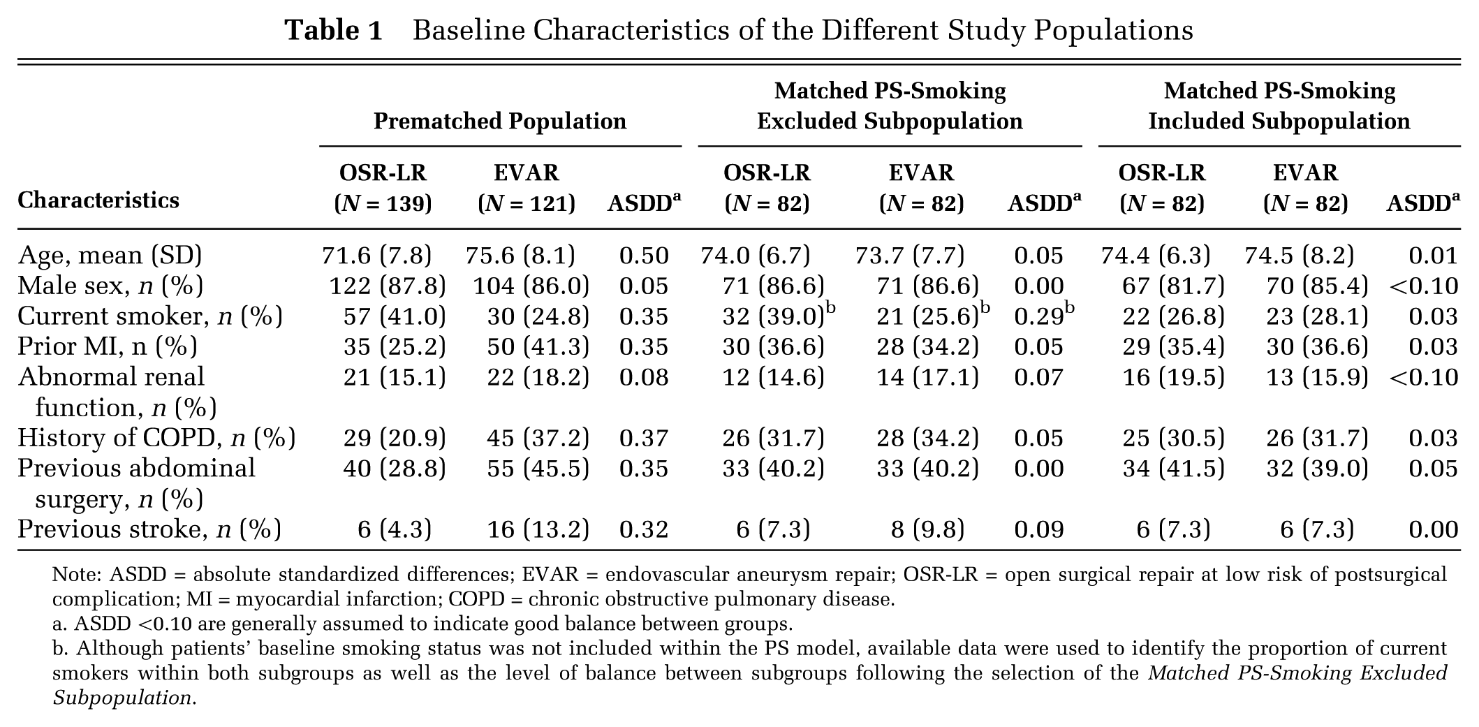
Note: ASDD = absolute standardized differences; EVAR = endovascular aneurysm repair; OSR-LR = open surgical repair at low risk of postsurgical complication; MI = myocardial infarction; COPD = chronic obstructive pulmonary disease.

ASDD <0.10 are generally assumed to indicate good balance between groups.

Although patients’ baseline smoking status was not included within the PS model, available data were used to identify the proportion of current smokers within both subgroups as well as the level of balance between subgroups following the selection of the Matched PS-Smoking Excluded Subpopulation.

Description of the Matched PS-Smoking Excluded Subpopulation

Patients’ individual PS were estimated using the PS-Smoking Excluded model for all individuals included within the Prematched Population. Six patients (2.3%) had PS based on the PS-Smoking Exclude model in nonoverlapping regions and were excluded from the analysis. Among the remaining 254 patients, we matched 82 patients (32.3%) assigned to the OSR-LR group to the 82 patients (32.3%) assigned to the EVAR group; selected patients formed the Matched PS-Smoking Excluded Subpopulation (Figure 1). This subcohort was composed of 142 males (86.6%), and the average age was 73.9 (7.2) years (Table 1). Balance within the Matched PS-Smoking Excluded Subpopulation was achieved in all examined covariates except one (i.e., patients’ smoking status at baseline [ASDD = 0.29]); this was to be expected since this covariate was not included within the PS-Smoking Excluded model, thus mimicking an unmeasured confounder.¹⁵

Description of the Matched PS-Smoking Included Subpopulation

Patients’ individual PS were estimated using the PS-Smoking Included model for all individuals included within the Prematched Population. Four patients (3.8%) had PS based on the PS-Smoking Included model in nonoverlapping regions and were excluded from the analysis. Among the remaining 256 patients, we matched 82 patients (32.0%) assigned to the OSR-LR group to the 82 patients (32.0%) assigned to the EVAR group; selected patients formed the Matched PS-Smoking Included Subpopulation (Figure 1). This subcohort was composed of 137 males (83.5%), and the average age was 74.5 (7.3) years (Table 1). Unlike the other study populations, balance was achieved on all eight baseline covariates within the Matched PS-Smoking Included Subpopulation.

Cost-Effectiveness Analyses

Base case estimates and 95% CI of the economic evaluation comparing EVAR to OSR within the two matched subpopulations are shown in Table 2. Results indicate that the incremental cost increased from $15,805 (95% CI = $12,985 to $18,751) when adjusting for all covariates except for baseline smoking status to $16,821 (95% CI = $14,234 to $19,505) when fully adjusting for all eight covariates. However, the incremental effectiveness decreased from a high of 0.10 LYG (95% CI = 0.05 LYG to 0.15 LYG) when adjusting for all covariates except for baseline smoking status to a low of 0.07 LYG (95% CI = 0.02 LYG to 0.12 LYG) when fully adjusting for all eight covariates. These incremental costs and effectiveness translated into an ICER estimated at $157,909 per LYG (95% CI = $97,819 per LYG to $320,006 per LYG) when adjusting for all covariates except baseline smoking status to an ICER estimated at $235,074 per LYG (95% CI = $131,600 per LYG to $675,804 per LYG) when fully adjusting for all eight covariates. Similar tendencies regarding the value of EVAR over OSR can be observed within the cost-effectiveness acceptability curves (Figure 2).

Table 2

Incremental Cost-Effectiveness Ratios Among the Two Matched Study Populations^a

	Matched PS-Smoking Excluded Subpopulation		Matched PS-Smoking Included Subpopulation
	OSR-LR	EVAR	OSR-LR	EVAR
1-Year cost	$18,421 ($16,970 to $20,113)	$34,227 ($32,172 to $36,574)	$17,945 ($16,565 to $19,489)	$34,766 ($32,597 to $37,173)
Incremental cost		$15,805 ($12,985 to $18,751)		$16,821 ($14,234 to $19,504)
1-Year effectiveness	0.89 (0.83 to 0.93)	0.99 (0.97 to 1.00)	0.91 (0.86 to 0.95)	0.98 (0.96 to 0.99)
Incremental effectiveness		0.10 (0.05 to 0.15)		0.07 (0.02 to 0.12)
Incremental cost-effectiveness ratio^b		$157,909 ($97,819 to $320,006)		$235,074 ($131,600 to $675,804)

Note: 95% CI = 95% bootstrapped confidence interval; EVAR = endovascular aneurysm repair; OSR-LR = open surgical repair at low risk of postsurgical complication.

All results represent the average and 95% bootstrapped pointwise confidence intervals.

Incremental cost-effectiveness ratio comparing EVAR to OSR. Results are presented as cost per life-year gained.

Figure 2

Cost-effectiveness acceptability curves comparing endovascular aneurysm repair to open surgical repair within the two matched study populations. PS = propensity score.

Discussion

As expected, measured confounding was shown to be present within the Prematched Population (Table 1), and as such, any ICER estimated within this study population would tend to be biased; further confounding adjustment would be required in order to obtain unbiased results. Results obtained in Table 1 show that matching on the PS-Smoking Included model improved the level of balance within all measured baseline characteristics that would tend to lead to less biased results within the Matched PS-Smoking Included Subpopulation than within the unmatched population.⁶ However, unlike randomization, PS methods can only adjust for measured confounding¹⁵; remaining unmeasured confounding could substantially bias the results of an economic evaluation based on nonrandomized data. Indeed, in our empirical example, unmeasured confounding due to the omitted confounder (i.e., patients’ baseline smoking status) may have biased the results in favor of EVAR (ICER estimated within the Matched PS-Smoking Excluded Subpopulation was $157,909 per LYG [95% CI = $97,819 per LYG to $320,006 per LYG] compared to the ICER estimated within the Matched PS-Smoking Including Subpopulation which was $235,074 per LYG [95% CI = $131,600 per LYG to $675,804 per LYG]). Alternatively, the ICER obtained within the Matched PS-Smoking Excluded Subpopulation could be viewed as being biased by Bias_UC and Bias_UE (Equation 5), whereas results obtained within the Matched PS-Smoking Included Subpopulation would be further adjusted for these biases.

Despite the fact that the focus of this study was to illustrate the impact of unmeasured confounding within an economic evaluation based on nonrandomized data, our results also provide an interesting example of the added complexity of confounding adjustment within economic evaluations based on nonrandomized data. Unlike comparative effectiveness studies or costing evaluations, full economic evaluations (as defined by Drummond and others³⁹) are bidimensional in nature, examining both the incremental cost in relation to the incremental effectiveness of one technology over another. In the context of an economic evaluation based on randomized data, the estimated ICER can be considered to be unbiased by measured and unmeasured confounders since both the incremental cost and the incremental effectiveness components are both considered to be unbiased by confounders due to the randomization process. This is not the case when the economic evaluation is based on nonrandomized data. As described by Kreif and others,⁴⁰ confounding within an economic evaluation based on nonrandomized data may either bias only the incremental cost component, only the incremental effectiveness component, or both. In nonrandomized studies, measured and unmeasured confounders can bias the incremental cost and/or the incremental effectiveness components of the ICER. Even if measured confounders can be dealt with the use of PS when conducting economic evaluations based on nonrandomized data, the bias due to unmeasured confounders still remains,¹⁵ a limit that is common to other frequently used confounding adjustment methods (e.g., multivariate regressions, covariate matching).^13,14 Of course, while this analysis focusses on cost per LYG, economic evaluation focusing on cost per quality-adjusted life-years gained can be limited by the same issues.

Our empirical example has identified an additional issue regarding confounding that has been rarely discussed in the context of economic evaluations based on nonrandomized data. In our empirical example, patients’ smoking status seems to confound both components of the ICER (Table 2). As discussed previously, other confounders could affect only one of the two components of the ICER. We are unable to state which of the three types of confounders (i.e., those biasing only the incremental cost component, those biasing only the incremental effectiveness component, or those biasing both components) have the greatest impact on the economic results of a study using nonrandomized data. One may expect that the prevalence of the confounders (i.e., rare confounders tending to be less problematic than prevalent confounders) and their strength (i.e., weak confounders tending to be less problematic than strong confounders) are important factors influencing the impact of confounding bias on the estimated ICER. In addition, the impact of the confounding bias should also depend on the magnitude of the incremental cost or of the incremental effectiveness (i.e., small versus large); confounding bias being more likely to affect the interpretation of the ICER when the incremental cost and the incremental effectiveness components are small than when they are large. Future work combining both empirical examples and simulation studies focusing on this additional issue is required.

Despite the value of this example, our study does present several limitations. First, we chose to illustrate the impact of unmeasured confounding within economic evaluations based on nonrandomized data through the use of an empirical example in which the true ICER of EVAR over OSR is undefined instead of using a simulation study. While the use of a simulation study could have provided a true representation of the impact of an unmeasured confounder,^17–19 using an empirical example illustrates how an unmeasured confounder can truly affect the results of an economic evaluation based on nonrandomized data instead of being due to the parameters imposed by the investigators. Nonetheless, current work is underway to conduct a simulation study to better understand how confounding bias affects the ICER under various scenarios that encompass the wide range of potential confounding effects observed within nonrandomized economic evaluations (i.e., those affecting solely the incremental cost component, those affecting solely the increment effect component, and those affecting both components). Second, we only examined a single unmeasured confounder in a single setting; unmeasured confounding present in other settings may affect the results of the economic evaluations differently. Although true, selection of this measured confounder as an omitted confounder (i.e., patients’ baseline smoking status) was motivated by the fact that patients’ smoking status is frequently absent from administrative databases. Third, instead of illustrating the impact of an unmeasured confounder, we illustrated the impact of a measured confounder that was unadjusted for. As mentioned previously, adjustment for a truly unmeasured confounder would have had required obtaining additional information on the selected unmeasured confounder through the use of an internal validation study.²⁴ However, since PS can only adjust for covariates that are entered within the PS model,⁶ a measured confounder that was not adjusted for would tend to be similar to a true unmeasured confounder. Fourth, we cannot exclude the possibility that true unmeasured confounding due to covariates not recorded within our data set is present within this empirical example and that the results obtained within the Matched PS-Smoking Included Subpopulation remain biased (i.e., Bias_UC and Bias_UE due to other unmeasured confounder could still remain). Although such a possibility remains, it is important to note that this empirical example only served to illustrate the potential impact of unmeasured confounding within an economic evaluation based on nonrandomized data when using PS methods and not to identify the true incremental value of EVAR over OSR. Researchers aiming to conduct true economic evaluations based on nonrandomized data should consider different approaches to either capture additional sociodemographic data at baseline a priori or consider techniques to collect these data a posteriori despite traditional limits associated with these techniques.²⁴ Fifth, as detailed within our methods, patients with presence of either prior congestive heart failure or of a “hostile abdomen” were excluded from our analysis. Although warranted in this setting,³² it is important to note that any exclusion of patients from the study population would limit the external validity of the results. Similarly, such an issue would also arise following the exclusion of patients due to PS trimming. Fortunately, the limited external validity of our results is of less concern in this specific context due to the illustrative nature of our example but could be of concern within other empirical settings. Sixth, use of PS trimming within this empirical example could affect our results regarding the impact of the omitted confounder on the ICER. Indeed, trimming the Prematched Population on two distinct PS led to the trimming of two different subsets of patients that could have differently affected the results we observed. However, this potential issue would be expected to have a minimal impact due to the small number of patients trimmed within both arms (i.e., 6 and 4 patients were trimmed within the PS-Smoking Excluded model arm and within the PS-Smoking Included model arm [Figure 1]). Finally, we only examined the impact of unmeasured confounding within economic evaluations when using PS matching and cannot comment on its relative performance compared to other adjustment techniques (e.g., multivariate regressions, covariate matching, instrumental variables). Additional work, both empirical and simulation based, is needed in this area to compare the relative performance of these different techniques. Such future work may also be used to determine the bias associated with misspecifications of the PS model and how such bias propagates through the economic evaluations.

In conclusion, this empirical example illustrated the impact of unmeasured confounding within an economic evaluation based on nonrandomized data as well as the limits of confounding adjustment through PS methods. Although future economic evaluations based on nonrandomized data may use PS methods to adjust for measured confounding, we, like others,²⁰ recommend that researchers be aware of the limits regarding unmeasured confounding that we presented within our analyses. Furthermore, additional work acknowledging the bidimensional nature of economic evaluation based on nonrandomized data is required to assess the relative performance of all the different adjustment techniques regarding the impact of unmeasured confounding within such studies.

Footnotes

Acknowledgements

Jason R. Guertin has received a Pfizer Canada Inc. Postdoctoral Mentoree Award, the 2015–2016 Bernie O’Brien Post-Doctoral Fellowship Award, and a postdoctoral training award from the Fonds de recherche du Québec–Santé for work unrelated to this article.

References

Dreyer

Tunis

Berger

Ollendorf

Mattox

Gliklich

. Why observational studies should be among the tools used in comparative effectiveness research. Health Aff (Millwood). 2010;29(10):1818–25. doi:10.1377/hlthaff.2010.0666.

Shrank

Patrick

Brookhart

. Healthy user and related biases in observational studies of preventive interventions: a primer for physicians. J Gen Intern Med. 2011;26(5):546–50. doi:10.1007/s11606-010-1609-1.

Hannouf

Zaric

. Cost-effectiveness analysis using registry and administrative data. In: Zaric

, ed. Operations Research and Health Care Policy. Berlin: Springer; 2013. p 341–61.

Klungel

Martens

Psaty

. Methods to assess intended effects of drug treatment in observational studies are reviewed. J Clin Epidemiol. 2004;57(12):1223–31. doi:10.1016/j.jclinepi.2004.03.011.

Rovithis

. Do health economic evaluation using observational data provide reliable assessment of treatment effects?Health Econ Rev. 2013;3(1):21. doi:10.1186/2191-1991-3-21.

Rosenbaum

Rubin

. The central role of the propensity score in observational studies for causal effects. Biometrika. 1983;70(1):41–55. doi:10.1093/biomet/70.1.41.

D’Agostino

Jr D’Agostino

Sr . Estimating treatment effects using observational data. JAMA. 2007;297(3):314–6. doi:10.1001/jama.297.3.314.

Kurth

Walker

Glynn

. Results of multivariable logistic regression, propensity matching, propensity adjustment, and propensity-based weighting under conditions of nonuniform effect. Am J Epidemiol. 2006;163(3):262–70. doi:10.1093/aje/kwj047.

D’Agostino

Jr.

Propensity score methods for bias reduction in the comparison of a treatment to a non-randomized control group. Stat Med. 1998;17(19):2265–81.

10.

Austin

. The performance of different propensity-score methods for estimating relative risks. J Clin Epidemiol. 2008;61(6):537–45. doi:10.1016/j.jclinepi.2007.07.011.

11.

Austin

. The relative ability of different propensity score methods to balance measured covariates between treated and untreated subjects in observational studies. Med Decis Making. 2009;29(6):661–77. doi:10.1177/0272989X09341755.

12.

Austin

Mamdani

. A comparison of propensity score methods: a case-study estimating the effectiveness of post-AMI statin use. Stat Med. 2006;25(12):2084–106. doi:10.1002/sim.2328.

13.

Greenland

Pearl

Robins

. Confounding and collapsibility. Stat Sci. 1999;14:29–46.

14.

Greenland

Morgenstern

. Confounding in health research. Annu Rev Public Health. 2001;22:189–212. doi:10.1146/annurev.publhealth.22.1.189.

15.

Brooks

Ohsfeldt

. Squeezing the balloon: propensity scores and unmeasured covariate balance. Health Serv Res. 2013;48:1487–507. doi:10.1111/1475-6773.12020.

16.

Woolridge

. Econometric Analysis of Cross Section and Panel Data. Cambridge (MA): MIT Press; 2001.

17.

Faries

Peng

Pawaskar

Price

Stamey

Seaman

Jr.

Evaluating the impact of unmeasured confounding with internal validation data: an example cost evaluation in type 2 diabetes. Value Health. 2013;16(2):259–66. doi:10.1016/j.jval.2012.10.012.

18.

Handorf

Bekelman

Heitjan

Mitra

. Evaluating costs with unmeasured confounding: a sensitivity analysis for the treatment effect. Ann Appl Stat. 2013;7(4):2062–80. doi:10.1214/13-AOAS665.

19.

Stamey

Beavers

Faries

Price

Seaman

Jr.

Bayesian modeling of cost-effectiveness studies with unmeasured confounding: a simulation study. Pharm Stat. 2014;13(1):94–100. doi:10.1002/pst.1604.

20.

Kreif

Grieve

Sadique

. Statistical methods for cost-effectiveness analyses that use observational data: a critical appraisal tool and review of current practice. Health Econ. 2013;22(4):486–500. doi:10.1002/hec.2806.

21.

Tarride

Blackhouse

De Rose

. Should endovascular repair be reimbursed for low risk abdominal aortic aneurysm patients? Evidence from Ontario, Canada. Int J Vasc Med. 2011;2011:308685. doi:10.1155/2011/308685.

22.

Bowen

De Rose

Blackhouse

. Systematic Review and Cost-Effectiveness Analysis of Elective Endovascular Repair Compared to Open Surgical Repair of Abdominal Aortic Aneurysms: Final Report (Report No. HTA001-0703-02). Hamilton, Ontario, Canada: Program for Assessment of Technology in Health, St. Joseph’s Healthcare Hamilton, McMaster University; 2007.

23.

Tarride

Blackhouse

De Rose

. Cost-effectiveness analysis of elective endovascular repair compared with open surgical repair of abdominal aortic aneurysms for patients at a high surgical risk: a 1-year patient-level analysis conducted in Ontario, Canada. J Vasc Surg. 2008;48(4):779–87. doi:10.1016/j.jvs.2008.05.064.

24.

Sturmer

Glynn

Rothman

Avorn

Schneeweiss

. Adjustments for unmeasured confounders in pharmacoepidemiologic database studies using external information. Med Care. 2007; 45(10suppl 2):S158–65. doi:10.1097/MLR.0b013e318070c045.

25.

Medical Advisory Secretariat. Endovascular Repair of Abdominal Aortic Aneurysms in Low Surgical Risk Patients: An Evidence Update. Toronto, Ontario, Canada: Medical Advisory Secretariat; 2010.

26.

Ontario Health Technology Advisory Committee. OHTAC Recommendation: Endovascular Repair of Abdominal Aortic Aneurysms for Low Surgical Risk Patients. Toronto, Ontario, Canada: Ontario Health Technology Advisory Committee; 2010.

27.

Lindsay

. Canadian Society for Vascular Surgery consensus statement on endovascular aneurysm repair. CMAJ. 2005;172(7):867–8. doi:10.1503/cmaj.1041584.

28.

Faizer

DeRose

Lawlor

Harris

Forbes

. Objective scoring systems of medical risk: a clinical tool for selecting patients for open or endovascular abdominal aortic aneurysm repair. J Vasc Surg. 2007;45(6):1102–8. doi:10.1016/j.jvs.2007.02.036.

29.

Chaikof

Fillinger

Matsumura

. Identifying and grading factors that modify the outcome of endovascular aortic aneurysm repair. J Vasc Surg. 2002;35(5):1061–6.

30.

Hollier

Taylor

Ochsner

. Recommended indications for operative treatment of abdominal aortic aneurysms. Report of a subcommittee of the Joint Council of the Society for Vascular Surgery and the North American Chapter of the International Society for Cardiovascular Surgery. J Vasc Surg. 1992;15(6):1046–56.

31.

Brewster

Cronenwett

Hallett

Jr . Guidelines for the treatment of abdominal aortic aneurysms. Report of a subcommittee of the Joint Council of the American Association for Vascular Surgery and Society for Vascular Surgery. J Vasc Surg. 2003;37(5):1106–17. doi:10.1067/mva.2003.363.

32.

Crump

Hotz

Imbens

Mitnik

. Dealing with limited overlap in estimation of average treatment effects. Biometrika. 2009;96(1):187–99. doi:10.1093/biomet/asn055.

33.

Sturmer

Rothman

Avorn

Glynn

. Treatment effects in the presence of unmeasured confounding: dealing with observations in the tails of the propensity score distribution—a simulation study. Am J Epidemiol. 2010;172(7):843–54. doi:10.1093/aje/kwq198.

34.

Austin

. Optimal caliper widths for propensity-score matching when estimating differences in means and differences in proportions in observational studies. Pharm Stat. 2011;10(2):150–61. doi:10.1002/pst.433.

35.

Austin

. Balance diagnostics for comparing the distribution of baseline covariates between treatment groups in propensity-score matched samples. Stat Med. 2009;28(25):3083–107. doi:10.1002/sim.3697.

36.

Ali

Groenwold

Pestman

. Propensity score balance measures in pharmacoepidemiology: a simulation study. Pharmacoepidemiol Drug Saf. 2014;23(8):802–11. doi:10.1002/pds.3574.

37.

Mamdani

Sykora

. Reader’s guide to critical appraisal of cohort studies: 2. Assessing potential for confounding. BMJ. 2005;330(7497):960–2. doi:10.1136/bmj.330.7497.960.

38.

Austin

Small

. The use of bootstrapping when using propensity-score matching without replacement: a simulation study. Stat Med. 2014;33(24):4306–19. doi:10.1002/sim.6276.

39.

Drummond

Sculpher

Torrance

O’Brien

Stoddart

. Methods for the Economic Evaluation of Health Care Programmes. 3rd ed.Oxford: Oxford University Press; 2005.

40.

Kreif

Grieve

Radice

Sadique

Ramsahai

Sekhon

. Methods for estimating subgroup effects in cost-effectiveness analyses that use observational data. Med Decis Making. 2012;32(6):750–63. doi:10.1177/0272989X12448929.

Illustration of the Impact of Unmeasured Confounding Within an Economic Evaluation Based on Nonrandomized Data

Abstract

Keywords

Mathematical Framework

Methods

Case Study

Treatment Algorithm

Propensity Score Models

Statistical Analyses

Cost-Effectiveness Analyses

Results

Description of the Prematched Population

Description of the Matched PS-Smoking Excluded Subpopulation

Description of the Matched PS-Smoking Included Subpopulation

Cost-Effectiveness Analyses

Discussion

Footnotes

Acknowledgements

References