Sage Journals: Discover world-class research

Abstract

Studies examining the consequences of intergenerational income mobility for individuals often face challenges due to multicollinearity between origin, destination, and a mobility construct based on the origin-destination difference. This article introduces a novel conceptualization of mobility, termed “reachability mobility,” which is based on the “easiness” of achieving a particular origin-destination combination within a population. This approach contrasts with the traditional lattice-based conceptualization. Furthermore, this study proposes using copulas—a statistical tool that captures the dependence structure between incomes of two generations while remaining insensitive to their marginal distributions—to measure reachability mobility. When combined with a standard measure of mobility direction, this approach allows scholars to simultaneously estimate the effects of origin, destination, and mobility along with numerous other methodological advantages. An illustrative example is provided that investigates the effect of intergenerational income mobility on mental health status using data from the National Longitudinal Survey of Youth 1979.

Keywords

copula intergenerational income mobility mental health NLSY79

Social scientists have long been interested in the consequences of intergenerational socioeconomic mobility for an individual’s well-being, attitudes, and behaviors (e.g., Sorokin 1959). Most existing research has followed a relational approach to social positions, emphasizing class mobility derived from occupational or educational attainment (e.g., Blau and Duncan 1967; Breen and Ermisch 2024; Hout 1983; Mare 1991). Relatively few studies have investigated the social consequences of intergenerational income mobility, particularly at the individual level.¹ However, the past few decades have witnessed a rapid and widespread rise in income and wealth inequality in most Western countries due to technological and institutional changes and various forms of discrimination in the labor market (Aeppli and Wilmers 2022; Blanchet, Saez, and Zucman 2022; Engzell and Mood 2023; Pfeffer and Killewald 2018; Weeden and Grusky 2014; Western and Rosenfeld 2011). It has been widely documented that economic inequalities might hinder social mobility, characterized by the “Gatsby curve” (Krueger 2012). The intergenerational persistence of economic (dis)advantage has been prominently stylized as a fact (Bloome 2014a) indicating a decline in openness to social opportunities. Echoing the rising significance of economic inequality, many recent studies have used innovative approaches to showcase levels of intergenerational income mobility, such as rank-based measurements and group-based income trajectory methods. These explorations have provided new, although sometimes divergent, evidence (Bloome, Dyer, and Zhou 2018; Chetty et al. 2014; Engzell and Mood 2023; Song et al. 2022). Given both the empirical prominence of economic inequality and the persistent theoretical interest of social scientists in uncovering the levels of intergenerational income mobility, it is unsurprising that there is a scholarly motivation to address the scant research on its social consequences for individuals (Grusky and Weeden 2006; Sakamoto and Wang 2020).

A straightforward way to estimate the net effect of intergenerational income mobility is to fit a linear model regressing an outcome simultaneously on origin (O, family income), destination (D, adult income), and mobility (M, income mobility). This intuitive strategy, however, fails when M linearly covaries with O and D (Blalock 1966), that is, when M is constructed to be the difference between O and D. To circumvent this problem, several modeling strategies have been proposed by sociologists, such as the square additive model (SAM; Duncan 1966), the diamond model (DM; Hope 1971, 1975), the diagonal reference model (DRM; Sobel 1981, 1985), and the mobility contrast model (MCM; Luo 2021). Despite their wide applications in the context of social class mobility (especially the DRM),² these modeling strategies, unfortunately, are not readily deployable for revealing the effect of intergenerational income mobility due to the shortness of statistical modeling itself and the continuous nature of income (more discussions are presented in the following).

Against this background, we propose addressing this problem by conceptualizing mobility from a new perspective. Inspired by the intuitive idea that mobility from origin i to destination j is considered “easier” if a larger number of people in a population achieve this specific i–j transition, we introduce a novel concept called “reachability mobility.” This approach highlights distinct aspects of mobility compared to conventional lattice-based measures and circumvents identification challenges by being independent of both origin and destination. Following this new conceptualization, we propose a copula-based measure of reachability mobility. Copulas are nonlinear mathematical functions that describe the dependence structure between two or more variables, netting off their marginal influences. As outlined later, the estimated copula densities reveal the likelihood of making a specific transition from origin i to destination j, thus reflecting the extent of “reachability” of the mobility between these two points. Methodologically, the copula-based measure no longer suffers from the identification problem because it is free from linear covariation with family and adult incomes. As an individual-level construct,³ it is also germane to many sophisticated statistical models, enhancing empirical researchers’ analytical capacities. This approach is illustrated by examining the consequences of intergenerational income mobility on mental health using data from the National Longitudinal Survey of Youth 1979 (NLSY79; available at https://www.nlsinfo.org/content/cohorts/nlsy79).

The Identification Challenge and Existing Modeling-Based Strategies

The identification challenge when studying the effect of intergenerational mobility emerges when M linearly covaries with O and D. In terms of income mobility, this problem arises when income mobility is operationalized to be the arithmetic difference between family income (or ranking) and adult children’s income (or ranking). The resultant multicollinearity renders the net effect of income mobility unidentifiable. In the previous literature, several modeling-based strategies (i.e., through specific statistical model configurations) have been developed to deal with this concern, but primarily for the case of a discrete socioeconomic status (SES) measure.

The SAM proposed by Duncan (1966) adopts an interactive modeling strategy, operationalizing M to be the interaction between O and D. This model configuration is justified on the basis that one would not observe the mobility effect if the variations of the outcome for the mobile can be accounted for by the additive combination of O and D. Nevertheless, because the interaction term itself is correlated with O and D, whether or not the coefficient of the interaction term can be interpreted as the mobility effect has been debatable (Hope 1971, 1975). Compared with the SAM, the DM, proposed by Hope (1971, 1975), gives up the distinction between O and D. Instead, the DM introduces a term that is deemed to represent the common dimension of SES, which is measured by the average of O and D. As a result, the DM only includes two terms in the model when examining the mobility effect: One is the average of O and D, and the other is the difference between O and D. The DM no longer has the identification problem but at the expense of sacrificing estimates of the distinctive effects of O and D. Besides, the estimated mobility effect can be statistically spurious because the coefficient for the difference between O and D would always be nonzero as long as the effects of O and D on the outcome differ from each other (House 1978).

Compared with these modeling strategies, the DRM (Sobel 1981, 1985) is perhaps the most widely used model currently (e.g., Billingsley, Drefahl, and Ghilagaber 2018; Van der Waal, Daenekindt, and de Koster 2017). According to Sobel (1981:898, Model 3.4), the DRM parameterizes the outcome Y of individual k with O_i and D_j as:

Y_{i j k} = \sum_{i = 1}^{I} μ_{i i} p O_{i} + \sum_{j = 1}^{J} μ_{j j} (1 - p) D_{j} + γ {(O - D)}_{i j k} + ε_{i j k} .

(1)

In this model, μ_ii and μ_jj are the population means in the iith and jjth cells of the mobility table, p gauges their relative weights, ε_ijk is the random error, and the mobility effect is captured by $\hat{γ} .$ The DRM solves the identification problem by introducing the parameter p, that is, O is multiplied by p, and D is multiplied by 1 – p. By doing so, the design matrix for Model 1 is shifted to be [ $\tilde{O}, \tilde{D}, O - D$ ],⁴ where ${\tilde{O}}_{i} = p O_{i}$ , ${\tilde{D}}_{j} = (1 - p) D_{j},$ $\tilde{O}$ is the column vector of $\tilde{O_{i}}$ s, $\tilde{D}$ is the column vector of $\tilde{D_{j}}$ s, and $O - D$ is the column vector of O minus D. $O - D \neq \tilde{O} - \tilde{D},$ so the design matrix is no longer rank deficient, and the model is identifiable.

The configuration of the DRM assumes that the core members of a specific class or status group are the nonmobile because they stay the longest. Therefore, they serve as the reference to whom the mobile cases are compared. However, as noted by Luo (2021), this assumption is questionable in the case of large-scale mobility. For income mobility, some extra challenges also emerge. For instance, income is a continuous measure, so there can be a very limited number of individuals with the same income value or income ranking as their parents. Moreover, to what extent the “rare” nonmobile can be substantively deemed to represent the “core members” of a well-defined SES group can be questionable.

The reliance on the nonmobile is no longer a concern when using the MCM, an extension of the SAM (Luo 2021). Instead of using the interaction terms to represent the mobility effect, the MCM subtracts the interaction term between origin i and destination i from the interaction term of origin i and destination j. By doing so, a series of origin-specific contrasts of the interaction terms are constructed to gauge the mobility effect. Compared with the DRM, the MCM has the merits of revealing mobility heterogeneities and handling the case of large-scale mobility. However, the MCM is not directly applicable to intergenerational income mobility either. The interaction analysis between continuous variables routinely relies on model extrapolation to produce a parsimonious estimate (Aiken, West, and Reno 1991), and this would hamper the construction of the origin-specific contrasts in MCM. If we abandon model extrapolation, the number of interaction terms would be too huge to be manageable.

Thus far, we have reviewed various existing modeling-based strategies that share the commonality of intentionally building nonlinear models for the relationship between mobility, origin, and destination. However, this identification strategy is somewhat mechanical or even artifactual because the model configurations are often made for the sake of model identification. Despite model interpretations a posteriori, some of them still lack solid and well-grounded theoretical supports. Consequently, scholars using these methods often find the analytical results difficult to interpret or too restrictive for tackling more complex mobility scenarios. In response, this article shifts attention from statistical modeling to the more fundamental facets of mobility: conceptualization and measurement. As demonstrated in the following, we define mobility from a novel perspective, ushering in new strategies to circumvent the identification problem and gain additional methodological advantages.

Revisiting the Conceptualization of Mobility: From Lattice to Reachability

Conventional Lattice-Based Conceptualization of Mobility

An intuitive measure of mobility, as noted earlier, is the arithmetic difference between O and D. This is illustrated in Figure 1a. Without loss of generality, we configure three levels of O (1, 2, and 3) and three levels of D (1, 2, and 3). People whose O is 1 and D is 3 are deemed to reveal more substantial mobility (a larger value of the mobility variable) than those whose O is 1 and D is 2. The mobility variable constructed in this way is a “lattice-based measure.” By “lattice,” we refer to the schema of SES, such as the Goldthorpe class scheme (Erikson and Goldthorpe 1992) or an ordinal scale of educational attainment. The mobility variable defined as such is a lattice-based one because individuals are structurally embedded in a predefined SES lattice and the mobility is manifested by the move from one position to another on the scale of lattice. In other words, the extent of mobility is configured according to the interval between rungs on the “ladder” built on the lattice. If we see intergenerational income mobility from this perspective, the extent of income mobility per se is equal to the span of move along the income (or income quantile) scale across generations (e.g., Hertel and Groh-Samberg 2019).

Figure 1.

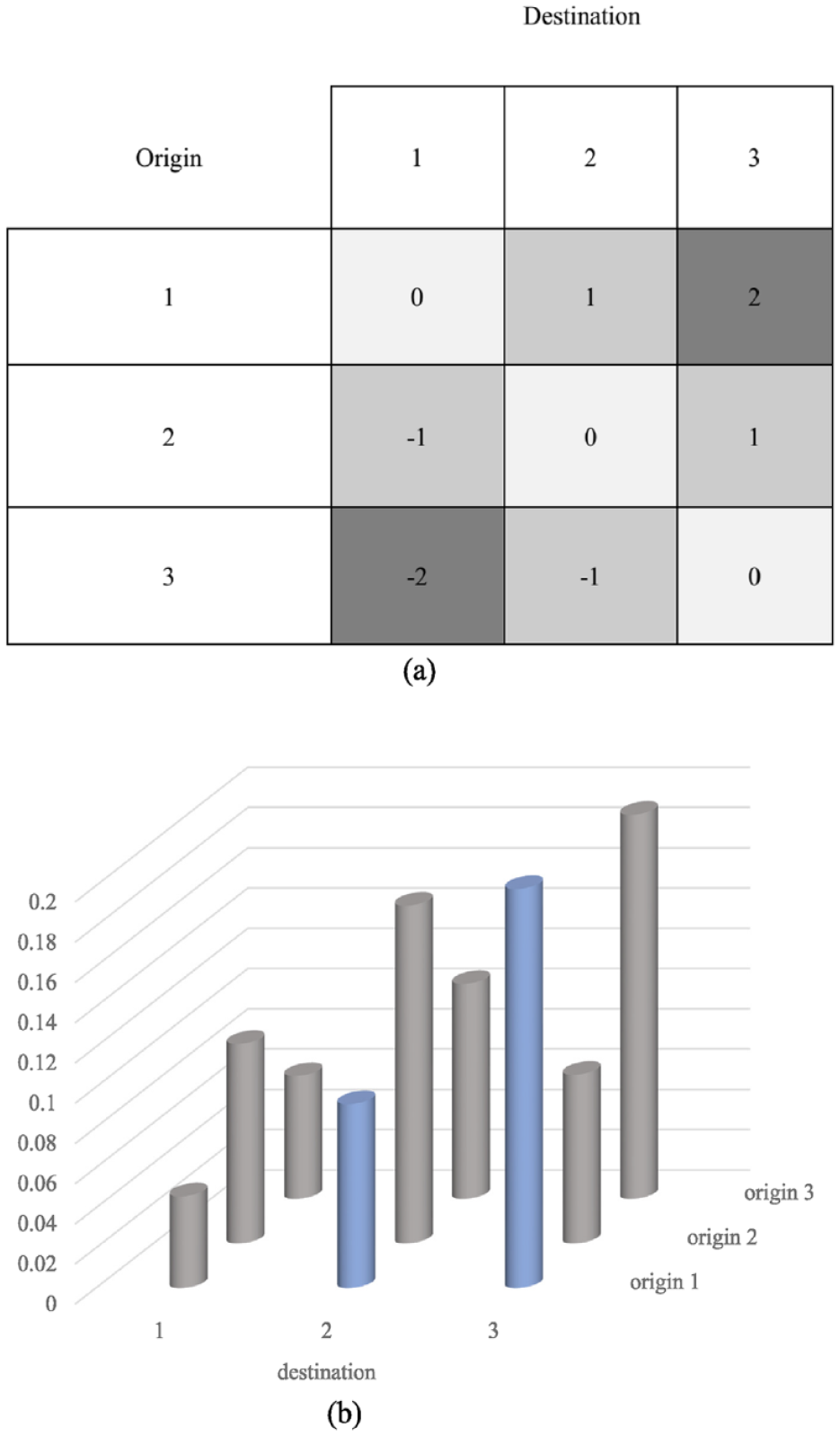
Conceptualizations of mobility: (a) lattice and (b) reachability.

Of course, some variants of this measure can be conceivable. For example, to circumvent the identification problem, one may use the absolute value of O – D. Let us temporarily put aside the direction measure of mobility (which we discuss later). |O – D| is still problematic because it suggests that one individual whose current income is $3,000 and family income is $2,000 has the exact extent of income mobility as another whose current income is $1,000 and family income is $2,000. This is an apparent limitation because it does not accommodate the fact that the $1,000 absolute income mobility occurs at different regions of the joint family—individual income distribution.⁵ In other words, the extent of difficulty of realizing this $1,000 absolute income mobility differs between these two scenarios. In this regard, one may follow a different line of thinking for constructing the mobility variable.

Reachability-Based Conceptualization of Mobility

In contrast to the lattice-based measure, this article proposes to conceptualize mobility from a different logic—reachability, which can thus be named the “reachability mobility.” The idea of reachability has been used to show the “closeness” between objects in a network (Wasserman and Faust 1994) or to detect outliers (Duan et al. 2009). By definition, strong reachability means that two objects can easily reach each other and thus appear together; weak reachability suggests more barriers for the two to “meet” each other, and thereby it represents higher social mobility distance from the perspective of reachability. Following this line of thinking, the mobility from a specific origin value i (O_i) to a particular value of destination j (D_j) is easier to reach for a given population if more individuals are observed to show the mobility pattern of O_i – D_j. Correspondingly, it indicates a lower level of social mobility distance from O_i – D_j. This idea is illustrated by Figure 1b, in which the longer the bar, the more likely to observe a specific O-D pair. For instance, the extent of reachability mobility from O₁ to D₃ is stronger than that from O₁ to D₂ because there are more people to mobilize from O₁ to D₃ than from O₁ to D₂. In other words, O₁ is less reachable to D₂ than to D₃ even though the lattice type of mobility suggests O₁ – D₂ is “easier” than O₁ – D₃ due to the shorter lattice distance (3 − 1 > 2 − 1).

To sum up, in the sense of reachability, mobility concerns how difficult to display a specific mobility pattern in a population, so for each individual, this measure informs us of the extent of being companioned when experiencing a particular mobility process. Note that the description of the reachability mobility illustrated in Figure 1 is “simplified” in the sense that SES is configured to have a limited number of levels. For intergenerational income mobility, the dynamics between continuous family and children’s incomes or income ranks would entail much more O-D pairs, each of which corresponds to an estimate of the extent of reachability that is not driven by the marginal family and children’s income distributions.⁶

Theoretical Justifications for the Reachability Mobility

We have now presented the idea of reachability mobility. This section further addresses the theoretical justifications for introducing this new conceptualization.

First, reachability mobility aligns more closely with sociological theories on social space and positioning. In Sorokin’s (1959) seminal work, for instance, social position is defined in terms of “relations toward all groups of a population” (Sorokin 1959:6), and “the location of a person’s position in this social universe is determined by establishing these relations” (Sorokin 1959:66). Following this line of argument, one’s socioeconomic positioning and its variations from one generation to another should be better understood in relation to the overall landscape of the income distribution across two generations. Reachability mobility exemplifies this because its value is precisely measured relative to all others. In contrast, the lattice approach defines mobility based on distances within a predefined lattice without considering the broader, “global,” and population-based situation of two generations’ incomes. Therefore, reachability mobility takes into account the population-level morphologies of income more carefully, making it more consistent with the sociological literature on social space and positioning.

Second, reachability mobility emphasizes one’s mobility status in comparison to others; thus, it is more consistent with existing theories that emphasize the importance of relative measures for accounting for social outcomes. One such case is the famous Easterlin’s paradox. As Easterlin (1995) suggests, an individual’s subjective well-being may not improve with increased absolute income if relative income remains unchanged. This rationale applies to research on intergenerational income mobility, where its influences depend not only on the absolute change in income across generations but also on the relative positions achieved through that income change. Indeed, upward income mobility may only marginally enhance (or potentially worsen) subjective well-being if it occurs against a backdrop of widespread upward income mobility during economic prosperity. This paradoxical scenario is often characterized by the term “frustrated achievers” (Zang and De Graaf 2016). Therefore, when analyzing the impact of intergenerational income mobility, especially on one’s subjective well-being, it is crucial to consider the overall relative likelihood of achieving specific mobility patterns, a perspective well captured by reachability mobility.

Third, reachability mobility uniquely addresses the classic dissociative thesis by correlating the alienation felt by individuals experiencing mobility with the relative number of peers in similar situations. In current literature, one long-standing approach to understanding the outcomes of mobility emphasizes the dissociative experiences stemming from the process itself, a concept with roots in Durkheim (1987) and Sorokin (1959). According to this theory, mobile individuals are detached from familiar routines and must adapt to the norms, values, and behaviors of their new social strata. The resulting identity conflicts, deprivation, anxiety, distress, and strain often make mobility detrimental to mental health (Luo 2021; Tolsma, De Graaf, and Quillian 2009). Intuitively, if many people within a population share the same mobility pattern, one’s sense of alienation tends to decrease due to the presence of more like-experienced peers (e.g., Buunk and Verhoeven 1991). This connection between feelings of alienation and the relative number of peers experiencing a specific mobility pattern is effectively illustrated by reachability mobility.

Paradigmatic Contrasts between the Two Conceptualizations of Mobility

The reachability mobility framework, as described earlier, represents a significant departure from the traditional lattice-based approach, which is summarized in Table 1. In essence, lattice-based mobility focuses on the distance between starting and ending points on the same socioeconomic scale. This “distance” of mobility is predetermined; for instance, moving from elementary school to college is considered a greater leap than moving from elementary school to junior high school. Therefore, lattice-based mobility is defined in a fixed and absolute manner by researchers. Consequently, it categorizes nonmobile cases as those where both generations occupy the same position on the lattice (diagonal cases in a mobility table). This conceptualization often leads to the issue of multicollinearity when considered together with both origin and destination. Additionally, the difference between origin and destination inherently indicates the direction of mobility because it compares the starting and ending points to determine whether the change is positive or negative.

Table 1.

Contrasts of Mobility Conceptualizations.

Lattice-Based Mobility	Reachability-Based Mobility
Difference of origin and destination on the same socioeconomic scale	The likelihood of observing a pair of particular combination of origin and destination
Configured a priori	Computed a posteriori
Nominal	Dynamic
Absolute	Relative
Collinear with origin and destination	Independent from origin and destination
Integrating mobility direction	Independent from mobility direction

In contrast, reachability mobility focuses on the probability of achieving a particular mobility outcome from origin to destination. This probability cannot be predetermined and has to be calculated or estimated after the fact. Therefore, reachability mobility does not categorize individuals into predefined groups of mobile or nonmobile but instead assesses each person’s relative ease of achieving a specific mobility status compared to others dynamically. This approach offers flexibility by highlighting the varying levels of difficulty in mobility and avoids grouping individuals with diverse mobility experiences into a single nominal category. This alternative conceptualization treats mobility independently of both origin and destination and does not encode information about the direction of mobility within the measure of reachability itself.

A simple example can show their distinctions. Imagine a scenario where the probability of attending college is forced to be 0.5 for the children’s generation (i.e., to toss a coin to determine the probability). We then would witness an empirical pattern where 50 percent of the children of parents with junior high school degrees grow up to have senior high school degrees (suppose a universal coverage of senior high school education) and 50 percent grow up to have bachelor’s degrees. In this case, the reachability mobility variable would be identical for these two trajectories. This identical “strength” of mobility makes sense in light of the fact that some social forces exist to equally divide the children’s generation into the two educational tracks insofar that the educational upward mobility into college is neither harder nor easier than the educational upward mobility into senior high school. By this fact, we mean senior high school and college education do not differ from each other in terms of the empirical “strength” of intergenerational mobility from junior high school. However, this kind of empirical “equivalence” between the two mobility trajectories is not able to be shown from the lattice-based perspective because the imposed lattice of educational gradient a priori assumes that the educational upward mobility into college is harder than the educational upward mobility into senior high school. Clearly, this is in conflict with the reality of the enforced 0.5 probability of college attendance.

Before moving to the next section, it is necessary to compare rank-based lattice mobility with reachability mobility. In rank-based lattice mobility, income rank is calculated relative to the income distribution of the respective generation. Thus, the rank-based lattice distance is also relative but focuses on the difference between two relative positions within their respective generations. In contrast, reachability mobility describes a specific mobility pattern, Oi – Dj, in terms of its likelihood to occur relative to all other mobility patterns. This relativeness is not based on a single generation’s situation but on the two-dimensional space created by both generations.

Empirical Relationship between the Two Conceptualizations of Mobility

The lattice and reachability conceptualizations approach mobility from distinct perspectives, necessitating a paradigmatic distinction between them. However, this divergence in theoretical framework does not imply that their empirical manifestations will invariably be in opposition. In general, individuals who achieve greater lattice mobility by overcoming more obstacles or experiencing more extreme life circumstances tend to exhibit limited reachability mobility because they represent only a relatively small portion of the population (Hertel and Groh-Samberg 2019). This scenario suggests a positive correlation between these two conceptualizations. A simple case in Figure 2a illustrates this point of view. Assuming a small scale of mobility where most individuals are located on the diagonal and the number of cases is negatively proportional to the lattice positions, the lattice mobility aligns with the reachability mobility, resulting in a correlation coefficient close to 1. Conversely, if the mobility scale is large and individuals primarily occupy the off-diagonal regions, the two conceptualizations would diverge, as shown in Figure 2b.

Figure 2.

Illustration of the empirical relationship between reachability and lattice: (a) small-scale mobility and (b) large-scale mobility.

Hence, empirically speaking, it is inappropriate to evaluate reachability mobility by comparing it with lattice mobility. Two implications follow. First, the empirical correlation between these two types of mobility largely depends on the specific research setting and the empirical data. Therefore, a strong correlation with lattice mobility does not render reachability mobility meaningless; rather, it provides insights into the mobility regime of that particular research setting. In other words, in some scenarios, reachability mobility might serve as a proxy for lattice mobility, but this is only one of many possibilities contingent on the specific research context. Second, if the empirical correlation between reachability and lattice mobilities is exceptionally strong, the two conceptualizations may overlap, resulting in multicollinearity. However, this multicollinearity, if detected, is driven by the characteristics of the empirical data in the specific research scenario rather than by the construction of reachability mobility itself.

How to Measure Reachability Mobility? A Copula-Based Approach

Copula and Reachability Mobility

The term “copula” derives from the Latin word meaning link. In statistics, a copula, or copula function, captures a specific way of linking two or more univariate distributions. More technical details can be found in Appendix I. For now, it is sufficient to understand that the estimated copula density is a statistic reflecting the probability of observing various pairs of income rankings independent of the marginal distributions (i.e., family income distribution and adult children’s income distribution).⁷ In this article, we propose to use estimated copula densities to measure reachability mobility.

Specifically, the copula density measures the probability of observing a pair of incomes or income rankings among all pairs in the population while being insensitive to the marginal income distributions of parents and adult children. Intuitively, a higher density value indicates a greater likelihood of a particular pair of income rankings, making that specific pair more attainable for the population. Because previous studies define the mobility variable from the perspective of the “difficulty” of achieving upward mobility, we can compute the complement of the estimated copula density, that is, 1 minus the copula density,⁸ and use this quantity to measure reachability mobility. Readers should note that strictly speaking, the reachability mobility for a particular mobility pattern O_i – D_j should be $1 - \sum_{i = 1}^{n} c o p u l a d e n s i t y_{i},$ where there exist n individuals with the O_i – D_j mobility. However, due to the continuous nature of income, almost every individual could have a unique mobility pattern, making the estimated reachability mobility highly individualized.⁹

There is another way to see why 1 minus the copula density well reflects the essential meaning of reachability mobility. In the extreme case where mobility is equally likely to be observed for any income-ranking pair, people from any income origin can freely mobilize to any income destination. Because there exist no relative differences in mobility from one person to another, the mobility variable should be zero. This can be captured by our constructed measure of reachability mobility. Formally, the equal mobility from any O to any D suggests that the joint distribution of O and D, f(O, D), equals the product of their marginal distributions, that is, f(O) × f(D). From Appendix I, we know that $f (O, D) = c o p u l a \times f (O) f (D),$ so the copula density is exactly unity, and the measure of reachability mobility is thus zero.

The Merits of Copula-Based Measure of Reachability Mobility

Measuring reachability mobility using the estimated copula densities offers several methodological advantages.

Model identification

Using the complement of copula density to measure reachability mobility has the merit of circumventing the identification challenge. That is because the copula density, by definition, is not driven by the margins (Vuolo 2017). This point of view can be confirmed by the fact that the joint probability density function (PDF) of family income and adult income can be decomposed into two components (see Appendix I for more details): One refers to the product of the marginal distributions, and the other is the copula density. Because the arguments of copula densities are the cumulative distribution functions (CDFs), the estimated copula densities should be insensitive to the specifications of the marginal PDFs, a property that the current literature has acknowledged.¹⁰ In other words, the copula densities stand for a new source of information that does not degenerate to the marginal characteristics. Therefore, using the complement of estimated copula densities to construct the measure of reachability mobility circumvents the identification challenge.

Circulation mobility

The insensitivity to the margins also informs us why the copula-based measure better reveals the circulation mobility (Hauser and Featherman 1978; Torche 2011). “Circulation mobility” refers to the extent of differential access to life chances across adults born in different classes of families given fixed marginal distributions of both generations’ SES (Breen and Jonsson 2005).¹¹ Because copula density is a construct that is insensitive to both O and D, the copula-based approach should be congruent with circulation mobility and reflects the extent of social fluidity and openness.

Readers should distinguish circulation mobility from the so-called relative mobility used by economists. Relative mobility compares the income of adults from different family income backgrounds and is often contrasted with absolute mobility, which concerns the income of adults at a specific absolute level of family income. By definition, an increase in adult children’s income always increases the extent of absolute mobility, but this is not the case for relative intergenerational income mobility (Deutscher and Mazumder 2021). Clearly, the meaning of relative mobility differs from that of circulation mobility in the sociological sense. Therefore, it is unsurprising that economists can use copulas to study both absolute and relative income mobility (e.g., Berman 2018; Chetty et al. 2017).

Mobility heterogeneity

The extent of heterogeneity in individuals’ mobility processes deserves more research attention (Luo, 2021). This need is addressed by the copula-based approach, which provides an individual-level measure. Consequently, it becomes easier to demonstrate how mobility effects covary with individual-level covariates. This is an advantage compared to the routine aggregate measures of intergenerational income mobility, such as elasticity (e.g., Beller and Hout 2006; Bloome 2014, 2017; Chetty et al. 2014; Fox, Torche, and Waldfogel 2016).

Richer modeling strategies

With the individual-level construct of mobility, researchers can examine the mobility effect using a broader range of modeling strategies. For instance, the simulation-extrapolation method (SIMEX) can be used to assess the extent of measurement error in the copula-based construct. Additionally, analytical procedures designed to handle confoundedness, such as propensity score matching, can be adopted (Morgan and Winship 2015).

To sum up, the methodological advantages of adopting the copula-based measure include the following:

The copula-based mobility measure circumvents the challenge of identification.

Designed to handle multivariate continuous variables, such as income, the copula-based mobility measure avoids the information loss that occurs when discretizing family or adult income.

The copula-based mobility measure aligns more closely with the theoretical tradition of dynamic social space constructs, revealing relative income advantages and capturing the alienation experiences of the mobile in relation to relative companionship.

As an individual-level construct, the copula-based mobility measure accommodates population heterogeneity to a great extent, expanding the analytical horizon for researchers through the adoption of more diverse modeling strategies.

The copula-based mobility measure is not sensitive to margins, allowing its empirical findings to be interpreted in terms of circulation mobility.

The copula-based mobility measure does not inherently rely on specific types of cases (e.g., nonmobile cases), making it suitable for large-scale studies of intergenerational income mobility.

An Illustrative Example

Background

This study uses the copula-based method to analyze how intergenerational income mobility affects one’s mental health status. The relationship between mobility status and subjective well-being is an enduring research question for sociologists (Durkheim 1987; Sorokin 1959), and the current literature underscores three perspectives (Houle 2011). The dissociative perspective views mobility as a source of stress, so regardless of the direction of mobility, the net effect of mobility should be negative (e.g., Houle and Martin 2011). The falling-from-grace perspective hypothesizes that only downward mobility as an involuntary failure is negatively correlated with one’s subjective well-being by evoking feelings of self-blame (Newman 1999). The acculturation perspective posits that it is the current SES that shapes one’s status of mental health, so mobility has no significant effects on one’s mental health (Blau 1956).

Despite our appreciation of these insights, most previous empirical studies use a categorical measure of SES. Rarely studies have paid serious attention to the income aspect of intergenerational advantage transmission. This is unfortunate in light of the burgeoning academic interest in the monetary measures of SES (Grusky and Weeden 2006; Sakamoto and Wang 2020). With the increasing availability of administrative data on income, there are good reasons to expect intergenerational income mobility to figure prominently (e.g., Beller and Hout 2006; Bloome 2014, 2017; Fox et al. 2016), so it is pressing to put the income-mental health nexus on the research agenda of sociologists. In this illustrative example, we draw on the NLSY79 to study the consequence of intergenerational income mobility on one’s mental health status (Boyle, Norman, and Popham 2009).

Sample and Measures

In the NLSY79, a random sample of people ages 14 to 22 was collected in 1979, and they were interviewed annually through 1994 and biennially thereafter. This research design facilitates the analysis of intergenerational mobility’s consequences by presenting family income in childhood and individual income in adulthood. This article concerns the period between 1978 and the year when the respondent was age 50 because the question about mental health was asked when the respondent had turned or was about to turn 50. To obtain reported parents’ income without overrepresenting late home-leavers, we follow previous studies to exclude respondents older than 19 in 1979 (Bloome 2014). After leaving out a fraction of cases with missing variables,¹² the final sample size is 4,068.

The specific measures of the variables used in this example are listed in the following.

Mental health status

We use the mental health components (MHC) score from the SF-12 Health Scale (original scale) to measure one’s mental health status. This scale covers a wide range of issues per subjective well-being, such as role functioning and vitality, in the extended 50+ health module. The MHC score is created based on the manual by Ware, Kosinski, and Keller (1995), and a higher score tends to reveal better mental health. Interviewed biennially from 2008 and thereafter, each individual was successively interviewed to report their SF-12 Health Scale values after they turned 50 (e.g., for 1959–1960 birth cohorts, they first self-reported their SF-12 Health Scale answers in 2010), so the SF-12 Health Scale collected the mental health information of the NLSY79 cohorts from 2008 to 2016.

Family income and adult income

We choose to use family income instead of the father’s income due to the vital role of family income in the well-being of children (Bloome 2014). This variable includes labor market earnings, assets, and transfers from government and nongovernment programs. We adjust for inflation over the years according to the reference year 2018 using the core Consumer Price Index (CPI) Retroactive Series. Subsequently, we averaged the total family income from 1978 to 1982 (survey years 1979–1983) to curtail the influences of measurement error¹³ (Mazumder 2005) and then adjust for family needs by dividing it by the square root of the family size (Bloome et al. 2018). As for adult income, previous studies have suggested that individuals’ permanent income could be best measured when people are over 30 years old (Chetty et al. 2014; Haider and Solon 2006), so we averaged the CPI-adjusted annual income of adult respondents who were over 30 years old to 50.

Mobility variable

The complement of estimated copula densities measures reachability mobility. We first scale the density values to be between 0 and 1,¹⁴ an operation having no impact on the substantive patterns of the copula density, and then compute the reachability mobility as 1 minus the scaled copula densities.

Mobility direction

The direction of mobility refers to upward, downward, or null mobility (immobility) when comparing the incomes of two generations. Intuitively, this measure can be constructed as follows. First, compute the relative ranking of an individual’s income within their generation, which scales the range of both income variables to between 0 and 1. The higher one’s income, the smaller one’s ranking. Because the two variables are now on the same scale, we can compute their arithmetic difference—for example, the ranking of adult children’s income minus the ranking of family income. If the difference is positive, it indicates that the adult children’s income ranking (e.g., the fifth quintile) is lower than that of their parents (e.g., the second quintile), signifying downward mobility. Conversely, if the difference is negative, it suggests an upward direction of mobility. If the rankings are the same (the difference is zero), it indicates nonmobility.

The mobility direction constructed in this manner yields a limited number of cases where the income ranking is identical to that of the parents. This limitation is not problematic for the copula-based approach because it does not rely on the identification of a specific “nonmobile” group. However, researchers seeking to maintain a larger pool of nonmobile individuals might consider a more flexible definition of mobility direction. For example, nonmobile cases could be defined as those where the family income ranking is within a certain range of the adult children’s income ranking (e.g., within ±0.05) or vice versa.

In the NLSY79, when comparing the family income ranking to that of adults, we observe that the number of nonmobile individuals (those with the same ranking) is very small. Specifically, 28.05 percent of respondents experienced downward mobility, and 71.93 percent experienced upward mobility. The immobile population consisted of only two individuals. Consequently, mobility direction is operationalized as a binary variable, with 0 representing downward mobility and 1 representing upward mobility.

It is important to note that this measure of mobility direction, by construction, operates independently of the copula-based measure of reachability mobility. Intuitively, if the estimated copula densities represent the likelihood of joint occurrences of some mobility pattern, both for upward and downward mobility, experiencing intergenerational income mobility—whether alone or alongside many other fellows—would independently influence one’s mental health.

Control variables

We control for a series of covariates, including gender (1 = male, 0 = female), respondents’ age in 1979, their education attainment concerning schooling years, and ethnicity (1 = Hispanic, 2 = Black, 3 = non-Black and non-Hispanic).

The descriptive information of the variables used in this article can be found in Table 2. The detailed code for the subsequent analyses can be found in Appendix III.

Table 2.

Descriptive Statistics of the National Longitudinal Survey of Youth 1979 Data.

Variable	Mean	SD	Observations
Family characteristics
Parental income(ln), child age 14–19 in 1979	7.812	0.754	8,816
Education level of the mother	10.784	3.143	8,425
Education level of the father	10.863	3.888	7,637
Mother born in United States (%)	89.3	—	8,953
Father born in United States (%)	88.4	—	8,905
Reside in South age 14(%)	36.8	—	8,720
Reside in urban age14(%)	78.9	—	8,938
Adult characteristics
Age in 1979	16.697	1.65	8,969
Race(%)			8,969
Hispanic	16.69		1,497
Black	26.22		2,352
Non-Black and non-Hispanic	57.09		5,120
Male(%)	50.5	—	8,969
Educational attainment	13.058	2.554	8,968
Income age 30–50 (ln)	8.738	2.769	8,192
Mental health score age 50+	53.016	8.902	5,906

Analytical Results

Copula estimation and constructing the reachability mobility

We first estimate the copula function that best fits the data parametrically (for more information about estimation, see Appendix I). Among a list of candidate copula functions (0 = independence copula, 1 = normal copula, 2 = Student t copula [t copula], 3 = Clayton copula, 4 = Gumbel copula, 5 = Frank copula, 6 = Joe copula, 7 = Clayton-Gumbel copula, 8 = Joe-Gumbel copula, 9 = Joe-Clayton copula, and 10 = Joe-Frank copula), the one with the best fit (smallest Akaike information criterion [AIC] and Bayesian information criterion [BIC]) is the Student t copula with two parameters to be, respectively 0.37 and 24.97 (log likelihood = 301.69, AIC = −599.38, BIC = −586.38).¹⁵

The copula density laid out in Figure 3a shows that the density mass concentrates on the diagonal (i.e., more reachable), which is consistent with our intuition about the intergenerational persistence of SES (Erikson and Goldthorpe 1992; Hauser 1978). This persistence is especially salient at the two ends of the income ranking spectrum. The density masses are heavy when family and adult children’s income rankings are extraordinarily high or low. Relatively, it is rare to find much density mass for the cases of significant intergenerational income ranking transitions either upward or downward.

Figure 3.

Estimated copula density using data from the National Longitudinal Survey of Youth 1979: (a) parametric estimate, (b) nonparametric estimate, and (c) heat map of the reachability mobility.

We also estimate the copula density nonparametrically using the transformation local likelihood method for cross-validation (Geenens, Charpentier, and Paindaveine 2017). The bandwidth matrix is $(\begin{matrix} 0.71 & - 0.71 \\ 0.71 & 0.71 \end{matrix}) .$ For the resultant copula density, see Figure 3b (log likelihood = 318.93, AIC = −608.61, BIC = −513.49). Compared with the copula density estimated parametrically, the nonparametrically estimated one is almost identical, so we do not describe it in detail.

Based on the estimated copula density, we scale it to ensure a range between 0 and 1 and construct the reachability mobility, as illustrated using the heat map. Figure 3c shows that the reachability mobility varies significantly on the two-dimensional space of family income rank by adult income rank. This heterogeneity in mobility at the individual level makes it convenient to investigate the consequences of intergenerational income mobility on one’s mental health status using a wide range of statistical models, as shown in the following. Note that the estimated copula densities are not relative frequencies because the latter are also driven by the marginal distributions.

The effect of intergenerational income mobility on mental health status

When examining the effect of intergenerational income mobility on mental health status, we fit a series of linear models. For the detailed analytical results, see Table 3.

Table 3.

Detailed Results of the Median Regression for Mental Health (Copula-Based Mobility Distance).

	Mobility Direction Effect	Mobility Effect	Full Model: OLS	OLS: Downward Mobility	OLS: Upward Mobility	Full Model: Median Regression	Median Regression: Downward Mobility	Median Regression: Upward Mobility
Log family income	0.742** (0.231)	0.294(0.179)	0.771*** (0.231)	0.957* (0.396)	0.687(0.357)	0.247(0.209)	0.626(0.383)	0.172(0.296)
Log adult income	0.753*** (0.0675)	0.848*** (0.0602)	0.748*** (0.0675)	0.606*** (0.0809)	1.076*** (0.256)	0.890*** (0.0611)	0.644*** (0.0782)	1.068*** (0.212)
Race (Black)	0.231(0.331)	0.209(0.331)	0.249(0.331)	0.620(0.561)	0.160(0.392)	0.202(0.300)	0.270(0.543)	0.0379(0.325)
Race (non-Black and non-Hispanic)	−0.751* (0.316)	−0.755* (0.316)	−0.737* (0.316)	−0.494(0.497)	−0.855* (0.398)	−0.544(0.286)	−0.482(0.481)	−0.618(0.330)
Gender (male)	1.269*** (0.237)	1.448*** (0.235)	1.316*** (0.238)	0.938* (0.373)	1.292*** (0.306)	0.897*** (0.215)	0.840* (0.361)	0.809** (0.253)
Educational attainment	0.127* (0.0498)	0.161** (0.0493)	0.136** (0.0499)	0.267*** (0.0798)	−0.0687(0.0642)	−0.0343(0.0452)	0.118(0.0771)	−0.120* (0.0532)
Age in 1979	−0.0115(0.0705)	−0.0165(0.0706)	−0.0170(0.0705)	0.0542(0.108)	−0.0541(0.0908)	−0.0458(0.0639)	−0.0318(0.104)	−0.0117(0.0753)
Mobility direction (upward)	1.059*** (0.320)		1.039** (0.320)			−0.0932(0.290)
Copula-based mobility		4.277* (1.961)	4.092* (1.961)	−1.476(2.565)	16.19** (5.303)	7.221*** (1.776)	3.793(2.479)	10.19* (4.395)
Intercept	37.89*** (1.969)	36.87*** (2.546)	34.08*** (2.686)	35.60*** (4.021)	25.32*** (4.981)	40.51*** (2.433)	40.21*** (3.887)	37.33*** (4.129)
N	5,813	5,813	5,813	2,861	2,952	5,813	2,861	2,952
Adjusted R²	0.059	0.058	0.059	0.054	0.059
Pseudo R²						0.028	0.026	0.029

Source: Data are from the National Longitudinal Survey of Youth 1979.

Note: Standard errors are in parentheses. OLS = ordinary least squares.

p < .05. **p < .01. ***p < .001 (two-tailed tests).

The upward direction of mobility, when considered independently (without accounting for reachability mobility), significantly promotes one’s mental health status, which is intuitively understandable. Additionally, reachability mobility, when examined on its own, also serves as a promoting factor for mental health. The positive effects of both upward mobility direction and reachability mobility remain significant when included together in the full ordinary least squares (OLS) model. It is also noteworthy that in the full model, both family income and adult income contribute to one’s subjective well-being.

In addition to these models, we also conducted subsample analyses, fitting the OLS model separately for those experiencing downward and upward mobility. No significant effect of reachability mobility was found among individuals experiencing downward mobility. In contrast, the promoting effect of reachability mobility persisted for those experiencing upward intergenerational income mobility. These findings suggest that for individuals whose SES is better compared to their parents, greater reachability mobility correlates with enhanced subjective well-being. In other words, the extent of mobility distance, as measured by reachability, significantly impacts the well-being of the upwardly mobile. Conversely, downward intergenerational income mobility negatively affects mental health “once and for all,” because further downward mobility, measured by reachability, does not exacerbate this detrimental effect.

These findings do not support the classic dissociative hypothesis because the mobility effect on mental health is not uniformly negative but, rather, depends on the direction of mobility. Given the significant mobility effect observed, the empirical patterns also reject the acculturation hypothesis. In this context, our findings extend the falling-from-grace hypothesis by revealing the asymmetric effects of upward and downward mobility. Notably, the negative impact of mobility among the downwardly mobile does not correspond to the extent of alienation, as measured by reachability. This implies that the “mental scar” left by intergenerational income deterioration, once formed, is difficult to change.

As previously mentioned, a key advantage of the copula-based approach is its flexibility in applying a wide range of statistical models. To illustrate this, we employed the median regression model to examine the impact of intergenerational income mobility on median mental health status (Koenker and Bassett 1978; McGreevy et al. 2009). Our conclusion remains consistent: Reachability mobility shows a significant positive effect among those experiencing upward mobility. Additionally, current income consistently enhances one’s mental health status across all models used. This finding suggests that subjective well-being is strongly influenced by current SES, albeit constrained by family background once the pattern of intergenerational income mobility is taken into account. The significance of current income level for subjective well-being aligns with the acculturation thesis (Blau 1956).

Comparison with the lattice mobility

This section examines the empirical relationship between reachability mobility and lattice mobility. Lattice mobility is quantified as the absolute difference between log family income and log adult income. As shown in Figure 4, no clear linear patterns are observed between these two mobility measures for either upward or downward mobility. In fact, their Pearson correlation coefficients are relatively modest (0.31 and −0.11, respectively). These findings indicate that in the context of the NLSY79 data set, reachability mobility provides unique insights distinct from those derived from lattice mobility.

Figure 4.

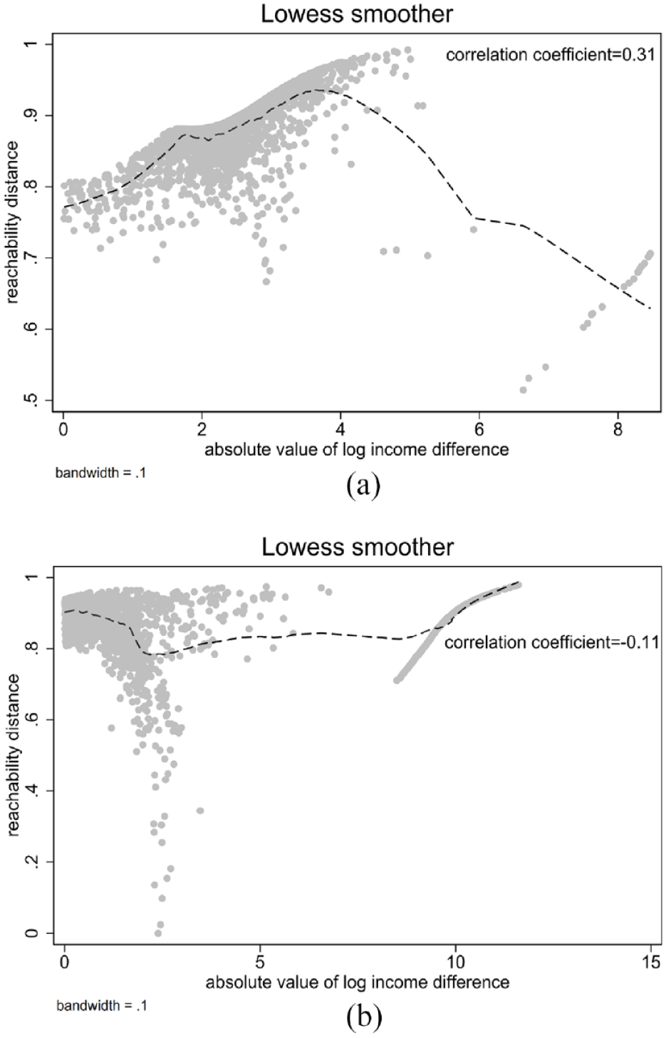
Relationship between reachability and lattice mobilities using the National Longitudinal Survey of Youth 1979 data: (a) the upward mobile and (b) the downward mobile.

We then repeat our multivariate analyses using the lattice mobility. For the empirical results, see Table 4. The effect of lattice mobility is always positive for the full OLS model, full median regression model, and the OLS model for the subpopulation of upward mobility, consistent with the results based on the reachability mobility. However, although the effect of reachability mobility is not statistically significant among the downwardly mobile (for both OLS and median regression models), the effect of the lattice mobility is surprisingly positive. That is counterintuitive and in conflict with the existing theoretical idea because this pattern suggests that when log adult income is smaller than log family income, the larger the gap, the happier one would be! Another thing to note is that when using the lattice measure of mobility, the estimated mobility effect among the upwardly mobile differs between the OLS and the median regression models, suggesting that the lattice mobility is more sensitive to the extreme values of the outcome than the reachability mobility.

Table 4.

Detailed Results of the Median Regression for Mental Health (Conventional Measure of Mobility Distance).

	Mobility Direction Effect	Mobility Effect	Full Model: OLS	OLS: Downward Mobility	OLS: Upward Mobility	Full Model: Median Regression	Median Regression: Downward Mobility	Median Regression: Upward Mobility
Log family income	0.742** (0.231)	0.764*** (0.184)	0.503* (0.230)	−0.0187(0.414)	0.562(0.334)	0.207(0.217)	0.399(0.400)	−0.417(0.301)
Log adult income	0.753*** (0.0675)	1.234*** (0.0710)	1.342*** (0.0913)	1.510*** (0.146)	1.397*** (0.192)	0.906*** (0.0861)	0.805*** (0.141)	1.431*** (0.173)
Race (Black)	0.231(0.331)	0.420(0.329)	0.418(0.329)	0.792(0.556)	0.191(0.392)	0.194(0.310)	0.374(0.539)	0.140(0.354)
Race (non-Black and non-Hispanic)	−0.751* (0.316)	−0.741* (0.313)	−0.750* (0.313)	−0.491(0.493)	−0.953* (0.398)	−0.583* (0.295)	−0.535(0.477)	−0.501(0.359)
Gender (male)	1.269*** (0.237)	0.759** (0.241)	0.774** (0.241)	0.348(0.371)	1.125*** (0.310)	0.606** (0.227)	0.303(0.359)	0.783** (0.280)
Educational attainment	0.127* (0.0498)	0.00492(0.0511)	0.00527(0.0511)	0.162* (0.0789)	−0.124(0.0656)	−0.0763(0.0481)	0.0252(0.0763)	−0.143* (0.0591)
Age in 1979	−0.0115(0.0705)	0.00114(0.0700)	0.00295(0.0700)	0.0589(0.107)	−0.0422(0.0909)	−0.0367(0.0660)	−0.0473(0.103)	0.00709(0.0819)
Mobility direction (upward)	1.059*** (0.320)		−0.687(0.367)			−0.398(0.346)
Absolute value of income difference		0.986*** (0.0999)	1.094*** (0.115)	1.320*** (0.179)	0.775** (0.252)	0.475*** (0.109)	0.371* (0.173)	−0.064(0.227)
Intercept	37.89*** (1.969)	33.52*** (1.887)	34.66*** (1.984)	34.08*** (3.253)	36.20*** (2.440)	46.79*** (1.870)	45.08*** (3.148)	47.24*** (2.200)
N	5,813	5,813	5,813	2,861	2,952	5,813	2,861	2,952
Adjusted R²	0.059	0.073	0.073	0.072	0.059
Pseudo R²						0.028	0.026	0.027

Source: Data are from the National Longitudinal Survey of Youth 1979.

Note: Standard errors are in parentheses. OLS = ordinary least squares.

p < .05. **p < .01. ***p < .001 (two-tailed tests).

In summary, compared to the lattice measure of mobility, the reachability measure of mobility, at least in the empirical example, offers the advantages of aligning with accumulated theoretical insights and being less influenced by modeling strategies. However, it is important for readers to recognize that these two measures reflect different conceptual frameworks. The comparison presented here serves primarily as an illustrative exposition.

Comparison with the DRM and MCM results

We also present the results using the DRM and MCM based on discretized measures of income. Readers should be cautious about this comparison because the copula-based method follows a different analytical logic from the DRM or the MCM, and the comparison presented here is simply for the illustrative purpose.

Specifically, we discretize both family income and adult income according to their quantiles, generating 10 groups for each variable. Using the categorical measures, we fit the DRM and the MCM. To enhance interpretation, we report the estimated effect on mental health for each cell of the 10 × 10 cross-table. For the results, see Figure 5.

Figure 5.

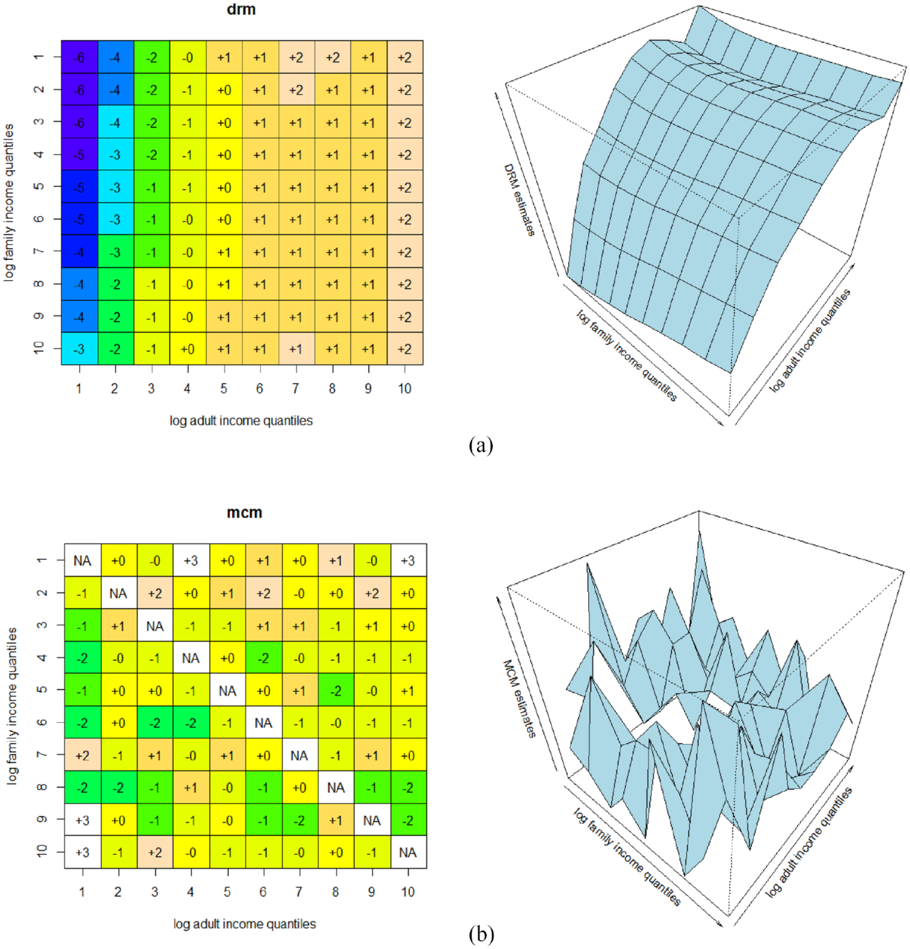
Results of the (a) diagonal reference model and (b) mobility contrast model based on income quantiles.

The DRM results suggest that locating at the lower quantiles of both family income and adult income, such as the cases at the upper-left corner of Figure 5, lowers one’s mental health status. Upward intergenerational income mobility promotes mental health, and more substantial downward intergenerational income mobility, defined as lattice mobility, hurts one’s subjective well-being.¹⁶ All of these results are consistent with those obtained by the copula-based method.

However, readers should note that the mobility effects suggested by Figure 5 may not be statistically robust. Indeed, the arithmetic difference between family income and adult income, used as a measure of mobility, fails to achieve statistical significance in the DRM model (estimate = −5.78, SE = 10.57, p > .1). It is important to recognize that this nonsignificant result pertains to the average scenario and does not account for potential heterogeneity that could be uncovered by the copula-based approach. Another consideration is that DRM results are based on comparisons with diagonal cells, inherently different from the logic of the copula-based method, which does not rely on predefined cells.

The results from the MCM do not exhibit a clear pattern given that most of the estimated effects are not statistically significant at the .05 level. This discrepancy from the results of DRM is puzzling, and a more detailed investigation is beyond the scope of this study. However, one conjecture is the complex modeling strategy of MCM, which involves overloaded interactions between discretized incomes of the two generations, one factor that tremendously consumes the freedom of statistical modeling.

Other supplementary analyses

In addition to the main findings, other additional analyses are performed. First, the results from SIMEX indicate that uncertainties or errors in copula density estimation are not a significant concern. Second, analytical results using generalized propensity score weighting affirm the robustness of the aforementioned findings against potential confounding from observed covariates. For further details, see Appendix II.

Conclusion and Discussions

The persistence or transition in SES across generations has been a significant social force influencing various aspects of individuals’ lives. This reality underscores the importance of research into the consequences of intergenerational mobility. Given the growing importance of income or earnings in assessing one’s SES, investigating the effects of intergenerational income mobility is academically and practically imperative.

However, in comparison to the extensive literature describing the basic patterns of intergenerational income mobility, there has been limited attention given to examining its individual-level effects. This gap primarily stems from the challenge posed when the measure of mobility linearly covaries with both family and adult children’s incomes, a concern not directly addressed by existing modeling strategies developed within sociology. Against this backdrop, this study seeks to address this issue by reconsidering the conceptualization of mobility. Specifically, it proposes a reachability-based conceptual framework that emphasizes the intuitive notion that mobility from Oi to Dj should be considered significant if it is more achievable, a concept easily quantifiable by the likelihood of observing the Oi – Dj combination in a population net of marginal income distributions. The distinctiveness of reachability mobility is explored in contrast to the conventional lattice-based conceptualization.

To align with reachability mobility, we propose using the complement of estimated copula densities to measure its empirical manifestations. This approach offers several advantages. For instance, estimated copula densities are robust against variations in the marginal distributions of both origin and destination and facilitate the independent assessment of how origin, destination, and circulation mobility influence specific outcomes.

Illustratively, we apply this methodology using the NLSY79 data set to investigate the relationship between intergenerational income mobility and mental health status. Among those experiencing downward mobility, no significant net mobility effect (reachability mobility) is observed, whereas a positive effect on mental health is evident among the upwardly mobile. In addition to mobility effects, subjective well-being consistently benefits from higher current income rankings (destination). These findings withstand estimation errors in copula densities and potential confounding from observed covariates.

Copulas have become a well-established analytical tool in statistics, geography, and finance. Therefore, the method introduced in this article is accessible and practical for social and behavioral researchers. Moreover, copula methods offer extensive flexibility for extension. Recent studies on intergenerational mobility have increasingly shifted focus from the traditional two-generation scenario to include three generations—grandparents, parents, and adults (Mare 2014). Despite the added complexity of analyzing mobility patterns across three generations, copula techniques, particularly vine copulas (Czado 2019), are well-suited to handle such scenarios. This suggests a promising avenue for future research to explore income mobility across multiple generations using sophisticated copula methodologies.

Footnotes

Appendix I: Overview of Copulas

Appendix II: Detailed Results of the Supplementary Analyses

Appendix III: Code for Data Analyses (R and STATA)

# load necessary packages #

library(rgl)

library(copula)

library(psych)

library(MASS)

library(TwoCop)

library(foreign)

library(ggplot2)

library(VineCopula)

library(RoDiCE)

library(Rfast)

library(kdecopula)

set.seed(1)

# illustrate typical copulas #

par(mfrow=c(2,2),mar=c(3.2,3,1.2,0))

norm.cop <- ellipCopula("normal", param = c(.6),dim = 2, dispstr = "un")

persp(norm.cop, dCopula, theta = 40, zlab="",xlab ="x", ylab="y", cex.lab=1.3,main="Normal copula density")

clayton.cop <- archmCopula("clayton", param = c(3),dim = 2)

persp(clayton.cop, dCopula, theta = 40, zlab="",xlab ="x", ylab="y", cex.lab=1.3,main="Clayton copula density")

gumbel.cop <- archmCopula("gumbel", param = c(4),dim = 2)

persp(gumbel.cop, dCopula, theta = 40, zlab="",xlab ="x", ylab="y", cex.lab=1.3,main="Gumbel-Hougaard copula density")

frank.cop <- archmCopula("frank", param = c(5),dim = 2)

persp(frank.cop, dCopula, theta = 40, zlab="",xlab ="x", ylab="y", cex.lab=1.3,main="Frank copula density")

# generate copula density values #

setwd("F:\\Spring 2021\\copula and intergenerational income mobility")

dat=na.omit(read.dta("incomedata.dta"))

attach(dat)

Xo=cbind(pobs(lnfainc2), pobs(logavincome))

cop_original <- BiCopSelect(pobs(lnfainc2), pobs(logavincome), familyset = NA, indeptest = FALSE, level = 0.05, se= T)

plot(cop_original, xlab="log family income", ylab="log adult income")

contour(cop_original, xlab="log family income", ylab="log adult income")

plot(kdecop(Xo), xlab="log family income", ylab="log adult income")

contour(kdecop(Xo), xlab="log family income", ylab="log adult income")

fit=kdecop(Xo)

# using the estimated copula model to predict the density for each observed value #

dsty=dstyrowsum=dstycolsum=rep(NA,dim(Xo)[1])

for (i in 1:dim(Xo)[1]){

dsty[i]=dkdecop(Xo[i,], fit)

}

dsty=dsty/sum(dsty)

# move back to stata and merge with the predicted densities #

gen copuladistance=1-dsty/0.0010037

gen upwardmob=0

replace upwardmob=1 if rankadultincome>rankfamilyincome

label variable upwardmob "mobility direction (upward)"

label variable copuladistance "reachability mobility"

reg mental_health_50 lnfainc2 logavincome raceadult2 raceadult3 male edu age79 upwardmob

estimates store model1

reg mental_health_50 lnfainc2 logavincome raceadult2 raceadult3 male edu age79 copuladistance

estimates store model2

reg mental_health_50 lnfainc2 logavincome raceadult2 raceadult3 male edu age79 upwardmob copuladistance

estimates store model3

reg mental_health_50 lnfainc2 logavincome raceadult2 raceadult3 male edu age79 upwardmob copuladistance if upwardmob ==0

estimates store model4

reg mental_health_50 lnfainc2 logavincome raceadult2 raceadult3 male edu age79 upwardmob copuladistance if upwardmob ==1

estimates store model5

qreg mental_health_50 lnfainc2 logavincome raceadult2 raceadult3 male edu age79 upwardmob copuladistance, q(0.5)

estimates store model6

qreg mental_health_50 lnfainc2 logavincome raceadult2 raceadult3 male edu age79 upwardmob copuladistance if upwardmob ==0, q(0.5)

estimates store model7

qreg mental_health_50 lnfainc2 logavincome raceadult2 raceadult3 male edu age79 upwardmob copuladistance if upwardmob ==1, q(0.5)

estimates store model8

coefplot (model1), bylabel(direction effect (OLS))|| (model2), bylabel(mobility effect (OLS))|| (model3), bylabel(OLS full model)|| (model4), bylabel(DM(OLS))|| (model5), bylabel(UM (OLS))|| (model6), bylabel(median reg (full model))|| (model7), bylabel(DM(median reg))|| (model8), bylabel(UM(median reg)) drop(_cons) xline(0) nokey msize(vsmall) msymbol(Oh) xlabel(,labsize(vsmall)) mlabgap(*2) mlabel(cond(@pval<.001, "***", cond(@pval<.01, "**", cond(@pval<.05, "*", "")))) note("* p < .05, ** p < .01, *** p < .001") mlabcolor(red)

# relationship with routine measures of mobility #

lowess copuladistance logincomediffabs if upwardmob==1, ytitle("reachability distance") xtitle(absolute value of log income difference) msymbol(o) mcolor(gs12) bw(0.1)

pwcorr copuladistance logincomediffabs if upwardmob==1, sig

lowess copuladistance logincomediffabs if upwardmob==0, ytitle("reachability distance") xtitle(absolute value of log income difference) msymbol(o) mcolor(gs12) bw(0.1)

pwcorr copuladistance logincomediffabs if upwardmob==0, sig

# using the routine measure of mobility #

reg mental_health_50 lnfainc2 logavincome raceadult2 raceadult3 male edu age79 upwardmob

estimates store model1

reg mental_health_50 lnfainc2 logavincome raceadult2 raceadult3 male edu age79 logincomediffabs

estimates store model2

reg mental_health_50 lnfainc2 logavincome raceadult2 raceadult3 male edu age79 upwardmob logincomediffabs

estimates store model3

reg mental_health_50 lnfainc2 logavincome raceadult2 raceadult3 male edu age79 upwardmob logincomediffabs if upwardmob ==0

estimates store model4

reg mental_health_50 lnfainc2 logavincome raceadult2 raceadult3 male edu age79 upwardmob logincomediffabs if upwardmob ==1

estimates store model5

qreg mental_health_50 lnfainc2 logavincome raceadult2 raceadult3 male edu age79 upwardmob logincomediffabs, q(0.5)

estimates store model6

qreg mental_health_50 lnfainc2 logavincome raceadult2 raceadult3 male edu age79 upwardmob logincomediffabs if upwardmob ==0, q(0.5)

estimates store model7

qreg mental_health_50 lnfainc2 logavincome raceadult2 raceadult3 male edu age79 upwardmob logincomediffabs if upwardmob ==1, q(0.5)

estimates store model8

Funding

The author(s) disclosed receipt of the following financial support for the research, authorship, and/or publication of this article: The first author acknowledges the support from the national social science foundation (22VRC140) and Shanghai leading scholar program. Earlier versions benefit greatly from the comments and suggestions from Alexandra Cooperstock, Austen Mack-Crane, Barum Park, Benjamin Cornwell, Cody Reed, Erin York Cornwell, Fabian T. Pfeffer, Kelly Musick, Kim Weeden, Soul Han, Wonjeong Jeong, Xi Song, Xiang Zhou, Xiaogang Wu, and Yu Xie, as well as participants of the 2022 ASA annual meeting, 2022 CASER Research Workshop Series at NYU Shanghai, and 2024 RC 28 Section of Intergenerational Mobility and Inequality.

ORCID iDs

Anning Hu

Zhipeng Zhou

1

The current literature on intergenerational income mobility places much attention on the empirical description of the status of (im)mobility within a society (Björklund, Jäntti, and Lindquist 2009; Lee and Solon 2009), among a specific group of individuals (Harding and Munk 2020), or across different periods (Lee and Solon 2009; Palomino, Marrero, and Rodríguez 2018). There are also studies on the determinants for the pattern of intergenerational income mobility, such as economic institutions (Breen and Jonsson 2005; DiPrete and Grusky 1990; Esping-Andersen 1990; Mitnik, Cumberworth, and Grusky 2016), educational expansion (Lucas 2001; Raftery and Hout 1993; Torche 2011; Zhou 2019), demographic change (Andersson et al. 2009; Bloome 2017), and migration (Andersen 2016; Gautier, Svarer, and Teulings 2010). Relatively limited attention has been paid to the effect of intergenerational income mobility (one exception is Okamoto, Avendano, and Kawachi 2019, but some methodological concerns linger).

2

These methods have been widely used to examine the mobility effect on well-being (Houle and Martin 2011; Sorokin 1927; Zang and De Graaf 2016), political attitudes and behaviors (Tolsma, De Graaf, and Quillian 2009; Weakliem 1992), and demographic behaviors (Kasarda and Billy 1985; ).

3

Other measures of mobility, such as the income elasticity that has been widely used by economists, are gauged at an aggregate instead of individual level.

4

The original design matrix is [O, D, O-D], which is rank deficient one.

5

One may use income ranks, but the rank difference has the same problem.

6

Otherwise, the mobility construct would not be independent from O and D.

7

In this regard, the estimated copula densities differ from the observed relative frequencies due to this property of marginal insensitivity. In addition, the copula method has been mainly used to handle continuous variables; for categorical measures of socioeconomic, more sophisticated procedures need to be employed (). Hence, the copula methods cannot be directly used for the traditional mobility table analysis.

8

The copula density mass should be standardized between 0 and 1, so the complement is computed by 1 minus the estimated copula density mass.

9

For instance, in the following illustrative example, 8,038 distinct copula estimates are reported for 8,066 respondents.

10

For instance, to control the sensitivity to marginal distribution specifications, we may compute the rank-rank correlation, which is strongly related to copulas. In the economic literature, this property has been drawn on in studies such as .

11

In contrast, structural mobility is driven by grand sociopolitical changes (i.e., industrialization; e.g., ).

12

We tested several ways of handling the missing values, and the substantive conclusions remain the same.

13

The measurement error of income lies in that a snapshot measure of income at a particular period could poorly approximate the permanent income’s life course. In the current literature, there are two types of measurement errors. The first concerns only family income, also called the attenuation bias, the classic measurement error, or the errors-in-variable problem. To handle it, one may use instrumental variable (e.g., parental occupations; e.g., Cervini-Plá 2015) or average multiple waves of income measures (e.g., Chetty et al. 2014). This article follows the strategy of averaging family income over multiple years. The other measurement error concerns family and adult children’s income, also called the lifecycle bias (Grawe 2006). Haider and Solon (2006) point out that this error cannot be handled with the routine instrumental variable method, and controlling for age in a linear model offers little help. If extra information (e.g., multiple measures of income for each individual) is available, one may adopt the generalized errors-in-variable method developed by Nybom and Stuhler (2017) to adjust the estimands and curtail the influences of this problem, but this is a tall order because it is rare to get access to multiple measures of income at the same time. Therefore, in this example, we follow suggestion by averaging adult children’s income for multiple years.

14

The copula density can be formulated to be f(FI, CI) / [f(FI)f(CI)], so it is not always ranged between 0 and 1.

15

The Kendall’s τ corresponding to this copula is 0.22, with the p value <.01.

16

However, mild downward mobility may still positively correlate with mental health status, such as those from the 10th quantile family income to the 5th quantile adult income.

17

This model, however, assumes the independence between the estimation error and the random error term in the outcome model.

18

Note that the SIMEX method is used with the classic measurement error, where the measurement error is additive to the predictor.

19

However, the confoundedness due to unobserved covariates cannot be fixed in this way.

Author Biographies

Dr. Hu Anning is distinguished professor of sociology and vice dean of Graduate School at Fudan University, Shanghai, China. His research interests include social inequality, education, religion, trust, culture, and statistical methods. Dr. Hu has published over 100 academic articles and three monographs, with research appearing in major sociological outlets, such as Sociology-The Journal of the British Sociological Association, British Journal of Sociology, Journal of Marriage and Family, Chinese Sociological Review, Social Science Research, Poetics, Journal for the Scientific Study of Religion, and Research in Social Stratification and Mobility, to name a few.

Zhipeng Zhou is a PhD student in sociology at Cornell University. His research interest covers the various areas of inequality, organization and work, and labor market. His current research projects examine how the reorganization of work and its changing nature associate with the formation of labor market inequality amid the global trends in precarious work and technology innovation.

References

Aeppli

Clem

Wilmers

Nathan

. 2022. “Rapid Wage Growth at the Bottom Has Offset Rising US Inequality.” Proceedings of the National Academy of Sciences 119(42):1–7.

Aiken

Leona S.

West

Stephen G.

Reno

Raymond R.

1991. Multiple Regression: Testing and Interpreting Interactions. New York, NY: Sage.

Andersen

Hans Skifter

. 2016. “Spatial Assimilation? The Development in Immigrants’ Residential Career with Duration of Stay in Denmark.” Journal of Housing and the Built Environment 31(2):297–320.

Andersson

Gunnar

Rønsen

Marit

Knudsen

Lisbeth B.

Lappegård

Trude

Neyer

Gerda

Skrede

Kari

Teschner

Kathrin

, et al. 2009. “Cohort Fertility Patterns in the Nordic Countries.” Demographic Research 20(14):313–52.

Bearman

Peter S.

Deane

Glenn

. 1992. “The Structure of Opportunity: Middle-Class Mobility in England, 1548-1689.” American Journal of Sociology 98(1):30–66.

Beller

Emily

Hout

Michael

. 2006. “Intergenerational Social Mobility: The United States in Comparative Perspective.” The Future of Children 16(2):19–36.

Berman

Yonatan

. 2018. “The Evolution of Global Absolute Intergenerational Mobility.” Pp. 53–56 in The Legacy of Tony Atkinson in Inequality Analysis. https://www.lisdatacenter.org/wp-content/uploads/files/resources-LIS%202018%20Conference%20Proceedings.pdf.

Billingsley

Sunnee

Drefahl

Sven

Ghilagaber

Gebrenegus

. 2018. “An Application of Diagonal Reference Models and Time-Varying Covariates in Social Mobility Research on Mortality and Fertility.” Social Science Research 75:73–82.

Björklund

Anders

Jäntti

Markus

Lindquist

Matthew J.

2009. “Family Background and Income during the Rise of the Welfare State: Brother Correlations in Income for Swedish Men Born 1932–1968.” Journal of Public Economics 93(5):671–80.

10.

Blalock

Hubert M.

Jr.

1966. “The Identification Problem and Theory Building: The Case of Status Inconsistency.” American Sociological Review 31(1):52–61.

11.

Blanchet

Thomas

Saez

Emmanuel

Zucman

Gabriel

. 2022. “Real-Time Inequality.” Working Paper 30229. National Bureau of Economic Research, Cambridge MA.

12.

Blau

Peter M.

1956. “Social Mobility and Interpersonal Relations.” American Sociological Review 21:290–95.

13.

Blau

Peter Michael

Duncan

Otis Dudley

. 1967. The American Occupational Structure. New York, NY: Wiley.

14.

Bloome

Deirdre

. 2014a. “Income Inequality and Intergenerational Income Mobility in the United States.” Social Forces 93(3):1047–80.

15.

Bloome

Deirdre

. 2014b. “Racial Inequality Trends and the Intergenerational Persistence of Income and Family Structure.” American Sociological Review 79(6):1196–225.

16.

Bloome

Deirdre

. 2017. “Childhood Family Structure and Intergenerational Income Mobility in the United States.” Demography 54(2):541–69.

17.

Bloome

Deirdre

Dyer

Shauna

Zhou

Xiang

. 2018. “Educational Inequality, Educational Expansion, and Intergenerational Income Persistence in the United States.” American Sociological Review 83(6):1215–53.

18.

Boyle

Pau J.

Norman

Paul

Popham

Frank

. 2009. “Social Mobility: Evidence That It Can Widen Health Inequalities.” Social Science & Medicine 68(10):1835–42.

19.

Breen

Richard

Ermisch

John

. 2024. “The Effects of Social Mobility.” Sociological Science 11:467–88.

20.

Breen

Richard

Jonsson

Jan O.

2005. “Inequality of Opportunity in Comparative Perspective: Recent Research on Educational Attainment and Social Mobility.” Annual Review of Sociology 31(1):223–43.

21.

Buunk

Bram P.

Verhoeven

Koen

. 1991. “Companionship and Support at Work: A Microanalysis of the Stress-Reducing Features of Social Interaction.” Basic and Applied Social Psychology 12(3):243–58.

22.

Cervini-Plá

María

. 2015. “Intergenerational Earnings and Income Mobility in Spain.” Review of Income and Wealth 61(4):812–28.

23.

Charpentier

Arthur

Fermanian

Jean-David

Scaillet

Olivier

. 2007. “The Estimation of Copulas: Theory and Practice.” Pp. 35–64 in Copulas: From Theory to Application in Finance, edited by Rank

London: Risk Books.

24.

Chetty

Raj

Grusky

David

Hell

Maximilian

Hendren

Nathaniel

Manduca

Robert

Narang

Jimmy

. 2017. “The Fading American Dream: Trends in Absolute Income Mobility since 1940.” Science 356(6336):398–406.

25.

Chetty

Raj

Hendren

Nathaniel

Kline

Patrick

Saez

Emmanuel

. 2014. “Where Is the Land of Opportunity? The Geography of Intergenerational Mobility in the United States.” The Quarterly Journal of Economics 129(4):1553–623.

26.

Czado

Claudia

. 2019. Analyzing Dependent Data with Vine Copulas: A Practical Guide with R. Cham, Switzerland: Springer International Publishing.

27.

Deutscher

Nathan

Mazumder

Bhashkar

. 2021. “Measuring Intergenerational Income Mobility: A Synthesis of Approaches.” Working Paper No. WP-2021-09. Federal Reserve Bank of Chicago, Chicago, IL.

28.

DiPrete

Thomas A.

Grusky

David B.

1990. “Structure and Trend in the Process of Stratification for American Men and Women.” American Journal of Sociology 96(1):107–43.

29.

Duan

Lian

Lida

Liu

Ying

Lee

Jun

. 2009. “Cluster-Based Outlier Detection.” Annals of Operations Research 168(1):151–68.

30.

Duncan

Otis Dudley

. 1966. “Methodological Issues in the Analysis of Social Mobility.” Pp. 51–97 in Social Structure and Mobility in Economic Development, edited by Smelser

N. J.

Lipset

S. M.

New York, NY: Transaction Publishers.

31.

Durkheim

Emile

. 1987. Suicide. A Study in Sociology. New York, NY: Free Press.

32.

Easterlin

Richard

. 1995. “Will Raising the Incomes of All Increase the Happiness of All.” Journal of Economic Behavior and Organization 27(1):35–48.

33.

Engzell

Per

Mood

Carina

. 2023. “Understanding Patterns and Trends in Income Mobility through Multiverse Analysis.” American Sociological Review 88(4):600–26.

34.

Erikson

Robert

Goldthorpe

John H.

1992. The Constant Flux: A Study of Class Mobility in Industrial Societies. New York, NY: Clarendon Press.

35.

Esping-Andersen

Gøsta

. 1990. “The Three Political Economies of the Welfare State.” International Journal of Sociology 20(3):92–123.

36.

Fox

Liana

Torche

Florencia

Waldfogel

Jane

. 2016. “Intergenerational Mobility.” Pp. 528–554 in The Oxford Handbook of the Social Science of Poverty, edited by D. Brady Burton

L. M.

Oxford, UK: Oxford University Press.

37.

Gautier

Pieter A.

Svarer

Michael

Teulings

Coen N.

2010. “Marriage and the City: Search Frictions and Sorting of Singles.” Journal of Urban Economics 67(2):206–18.

38.

Geenens

Gery

. 2020. “Copula Modeling for Discrete Random Vectors.” Dependence Modeling 8(1):417–40.

39.

Geenens

Gery

Charpentier

Arthur

Paindaveine

Davy

. 2017. “Probit Transformation for Nonparametric Kernel Estimation of the Copula Density.” Bernoulli 23(3):1848–73.

40.

Grawe

Nathan D.

2006. “Lifecycle Bias in Estimates of Intergenerational Earnings Persistence.” Labor Economics 13(5):551–70.

41.

Grusky

David B.

Weeden

Kim A.

2006. “Does the Sociological Approach to Studying Social Mobility Have a Future? Pp. 85–108 in Mobility and Inequality: Frontiers of Research from Sociology and Economics, edited by Morgan

S. L.

Grusky

D. B.

Fields

G. S.

Redwood City, CA: Stanford University Press.

42.

Haider

Steven

Solon

Gary

. 2006. “Lifecycle Variation in the Association between Current and Lifetime Earnings.” American Economic Review 96(4):1308–20.

43.

Harding

David J.

Munk

Martin D.

2020. “The Decline of Intergenerational Income Mobility in Denmark: Returns to Education, Demographic Change, and Labor Market Experience.” Social Forces 98(4):1436–64.

44.

Hauser

Robert M.

1978. “A Structural Model of the Mobility Table.” Social Forces 56(3):919–53.

45.

Hauser

Robert M.

Featherman

David L.

1978. “Opportunity and Change”. New York: Academic.

46.

Hertel

Florian R.

Groh-Samberg

Olaf

. 2019. “The Relation between Inequality and Intergenerational Class Mobility in 39 Countries.” American Sociological Review 84(6):1099–133.

47.

Hofert

Marius

Kojadinovic

Ivan

Martin

Mächler

Yan

Jun

. 2019. Elements of Copula Modeling with R. Berlin/Heidelberg, Germany: Springer International Publishing.

48.

Hope

Keith

. 1971. “Social Mobility and Fertility.” American Sociological Review 36(6):1019–32.

49.

Hope

Keith

. 1975. “Models of Status Inconsistency and Social Mobility Effects.” American Sociological Review 40(3):322–43.

50.

Houle

Jason N.

2011. “The psychological impact of intragenerational social class mobility.” Social Science Research 40(3): 757–72.

51.

Houle

Jason N.

Martin

Molly A.

2011. “Does Intergenerational Mobility Shape Psychological Distress? Sorokin Revisited.” Research in Social Stratification and Mobility 29(2):193–203.

52.

House

James S.

1978. “Facets and Flaws of Hope’s Diamond Model.” American Sociological Review 43(3):439–42.

53.

Hout

Michael

. 1983. Mobility Tables. Thousand Oaks, CA: Sage.

54.

Kasarda

John D.

Billy

John O. G.

1985. “Social Mobility and Fertility.” Annual Review of Sociology 11(1):305–28.

55.

Kluve

Jochen

Schneider

Hilmar

Uhlendorff

Arne

Zhao

Zhong

. 2012. “Evaluating Continuous Training Programs by Using the Generalized Propensity Score.” Journal of the Royal Statistical Society, Series A: Statistics in Society 175(2):587–617.

56.

Koenker

Roger

Bassett

Gilbert

. 1978. “Regression Quantiles.” Econometrica 46(1):33–50.

57.

Krueger

Alan

. 2012. “The Rise and Consequences of Inequality.” Presentation to the Center for American Progress, January 12. https://obamawhitehouse.archives.gov/sites/default/files/krueger_cap_speech_final_remarks.pdf

58.

Lee

Chul-In

Solon

Gary

. 2009. “Trends in Intergenerational Income Mobility.” The Review of Economics and Statistics 91(4):766–72.

59.

Lucas

Samuel R.

2001. “Effectively Maintained Inequality: Education Transitions, Track Mobility, and Social Background Effects.” American Journal of Sociology 106(6):1642–90. doi:10.1086/321300.

60.

Luo

Liying

. 2021. “Heterogeneous Effects of Intergenerational Social Mobility: An Improved Method and New Evidence.” American Sociological Review 87(1):143–73.

61.

Mare

Robert D.

1991. “Five Decades of Educational Assortative Mating.” American Sociological Review 56(1):15–32.

62.

Mare

Robert D.

2014. “Multigenerational Aspects of Social Stratification: Issues for Further Research.” Research in Social Stratification and Mobility 35:121–28.

63.

Mazumder

Bhashkar

. 2005. “Fortunate Sons: New Estimates of Intergenerational Mobility in the United States Using Social Security Earnings Data.” The Review of Economics and Statistics 87(2):235–55.

64.

McGreevy

Katharine M.

Lipsitz

Stuart R.

Linder

Jeffrey A.

Rimm

Eric

Hoel

David G.

2009. “Using Median Regression to Obtain Adjusted Estimates of Central Tendency for Skewed Laboratory and Epidemiologic Data.” Clinical Chemistry 55(1):165–69.

65.

Mitnik

Pablo A.

Cumberworth

Erin

Grusky

David B.

2016. “Social Mobility in a High-Inequality Regime.” The ANNALS of the American Academy of Political and Social Science 663(1):140–84.

66.

Morgan

Stephen L.

Winship

Christopher

. 2015. Counterfactuals and Causal Inference. New York, NY: Cambridge University Press.

67.

Newman

Katherine S.

1999. Falling from Grace. Downward Mobility in the Age of Affluence. Berkeley: University of California Press.

68.

Nybom

Martin

Stuhler

Jan

. 2017. “Biases in Standard Measures of Intergenerational Income Dependence.” Journal of Human Resources 52(3):800–25.

69.

Okamoto

Shohei

Avendano

Mauricio

Kawachi

Ichiro

. 2019. “Intergenerational Income Mobility and Health in Japan: A Quasi-experimental Approach.” Social Science & Medicine 230:37–48.

70.

Palomino

Juan C.

Marrero

Gustavo A.

Rodríguez

Juan G.

2018. “One Size Doesn’t Fit All: A Quantile Analysis of Intergenerational Income Mobility in the U.S. (1980–2010).” The Journal of Economic Inequality 16(3):347–67.

71.

Pfeffer

Fabian

Killewald

Alexandra

. 2018. “Generations of Advantage. Multigenerational Correlations in Family Wealth.” Social Forces 96(4):1411–42.

72.

Raftery

Adrian E.

Hout

Michael

. 1993. “Maximally Maintained Inequality: Expansion, Reform, and Opportunity in Irish Education, 1921-75.” Sociology of Education 66(1):41–62.

73.

Sakamoto

Arthur

Wang

Sharron Xuanren

. 2020. “The Declining Significance of Occupation in Research on Intergenerational Mobility.” Research in Social Stratification and Mobility 70:100521. doi:10.1016/j.rssm.2020.100521.

74.

Sklar

1959. “Fonctions de répartition à n dimensions et leurs marges.” Publications de l’Institut Statistique de l’Université de Paris 8:229–31.

75.

Sobel

Michael E.

1981. “Diagonal Mobility Models: A Substantively Motivated Class of Designs for the Analysis of Mobility Effects.” American Sociological Review 46(6):893–906.

76.

Sobel

Michael E.

1985. “Social Mobility and Fertility Revisited: Some New Models for the Analysis of the Mobility Effects Hypothesis.” American Sociological Review 50(5):699–712.

77.

Song

Zang

Emma

Land

Kenneth C.

Zheng

Boyan

. 2022. “Intergenerational Income Mobility Table Revisited: A Trajectory Group Perspective.” Research in Social Stratification and Mobility 80:100713. doi:10.1016/j.rssm.2022.100713.

78.

Sorokin

Pitrim A

. 1927. “Social and Cultural Mobility.” New York: Free Press.

79.

Sorokin

Pitirim A.

1959. Social and Cultural Mobility. New York, NY: Free Press.

80.

Stefanski

Leonard A.

Cook

James R.

1995. “Simulation-Extrapolation: The Measurement Error Jackknife.” Journal of the American Statistical Association 90(432):1247–56.

81.

Tolsma

Jochem

Graaf

Nan Dirk De

Quillian

Lincoln

. 2009. “Does Intergenerational Social Mobility Affect Antagonistic Attitudes towards Ethnic Minorities?” The British Journal of Sociology 60(2):257–77.

82.

Torche

Florencia

. 2011. “Is a College Degree Still the Great Equalizer? Intergenerational Mobility across Levels of Schooling in the United States.” American Journal of Sociology 117(3):763–807.

83.

Van der Waal

Jeroen

Daenekindt

Stijn

de Koster

Willem

. 2017. “Statistical Challenges in Modeling the Health Consequences of Social Mobility: The Need for Diagonal Reference Models.” International Journal of Public Health 62(9):1029–37.

84.

Vuolo

Mike

. 2017. “Copula Models for Sociology: Measures of Dependence and Probabilities for Joint Distributions.” Sociological Methods & Research 46(3):604–48.

85.

Ware

John

Kosinski

Mark

Keller

Susan

. 1995. SF-12: How to Score the SF-12 Physical and Mental Health Summary Scales. 2nd ed. Boston, MA: The Health Institute, New England Medical Center.

86.

Wasserman

Stanley

Faust

Katherine

. 1994. Social Network Analysis: Methods and Applications. Cambridge, UK: Cambridge University Press.

87.

Weakliem

David L.

1992. “Does Social Mobility Affect Political Behaviour?” European Sociological Review 8(2):153–65.

88.

Weeden

Kim A.

Grusky

David B.

2014. “Inequality and Market Failure.” American Behavioral Scientist 58(3):473–91.

89.

Western

Bruce

Rosenfeld

Jake

. 2011. “Unions, Norms, and the Rise in US Wage Inequality.” American Sociological Review 76(4):513–37.

90.

Zang

Emma

Graaf

Nan Dirk De

. 2016. “Frustrated Achievers or Satisfied Losers? Inter- and Intragenerational Social Mobility and Happiness in China.” Sociological Science 3:779–800.

91.

Zhou

Xiang

. 2019. “Equalization or Selection? Reassessing the ‘Meritocratic Power’ of a College Degree in Intergenerational Income Mobility.” American Sociological Review 84(3):459–85.

The Effect of Intergenerational Income Mobility: Reachability-Based Conceptualization and Copula-Based Measurement

Abstract

Keywords

The Identification Challenge and Existing Modeling-Based Strategies

Revisiting the Conceptualization of Mobility: From Lattice to Reachability

Conventional Lattice-Based Conceptualization of Mobility

Reachability-Based Conceptualization of Mobility

Theoretical Justifications for the Reachability Mobility

Paradigmatic Contrasts between the Two Conceptualizations of Mobility

Empirical Relationship between the Two Conceptualizations of Mobility

How to Measure Reachability Mobility? A Copula-Based Approach

Copula and Reachability Mobility

The Merits of Copula-Based Measure of Reachability Mobility

Model identification

Circulation mobility

Mobility heterogeneity

Richer modeling strategies

An Illustrative Example

Background

Sample and Measures

Mental health status

Family income and adult income

Mobility variable

Mobility direction

Control variables

Analytical Results

Copula estimation and constructing the reachability mobility

The effect of intergenerational income mobility on mental health status

Comparison with the lattice mobility

Comparison with the DRM and MCM results

Other supplementary analyses

Conclusion and Discussions

Footnotes

Appendix I: Overview of Copulas

Appendix II: Detailed Results of the Supplementary Analyses

Appendix III: Code for Data Analyses (R and STATA)

Funding

ORCID iDs

1

2

3

4

5

6

7

8

9

10

11

12

13

14

15

16

17

18

19

Author Biographies

References