Sage Journals: Discover world-class research

Abstract

While a gradient between income and depression is well documented, associational estimates are subject to bias due to measurement errors, reverse causation, and other sources of confounding. Causal studies are few and report small and divergent estimates, even in their direction. But prior research has important limitations for causal inference, such as relying on comparisons between individuals sensitive to each other’s relative income or capturing only a subset of pathways through which income affects well-being. This study leverages longitudinal and genomic data to assess how much some known biases affect the income-depression gradient and to what extent the gradient might be reflective of a causal effect. Findings from three U.S. samples—representing early midlife, late midlife, and older adulthood—are suggestive of a beneficial effect of income on mental health, especially in late midlife and beyond. The results have implications for interpreting the nature of socioeconomic disparities in mental health.

Keywords

depression mental health income effect income-depression gradient income-health gradient life course

An inverse association between income and various indicators of mental health—including clinical depression, depressive symptoms, and other indices measuring psychological distress and negative affective well-being—is widely documented (Eaton et al. 2001; Heflin and Iceland 2009; Kessler 1982; Martikainen et al. 2003; Ross and Huber 1985; Stewart-Brown et al. 2015). However, the extent to which these estimates reflect a causal relationship is unclear. Estimating effects by controlling only for observed confounders (or no controls at all) in cross-sectional data is vulnerable to reverse causation and other sources of bias that would overestimate the true casual effect. On the other hand, the presence of certain other confounders can result in underestimation, and estimates based on current income may be further attenuated due to measurement error and temporary income fluctuations.

While innovative causal designs have been employed to address these issues, findings are divergent. In high-income countries, the mental well-being effects of winning the lottery—a dramatic, exogenous shock to material circumstances—range from positive to negative (Apouey and Clark 2015; Brickman, Coates, and Janoff-Bulman 1978; Gardner and Oswald 2007; Lindqvist, Östling, and Cesarini 2020; Raschke 2019).¹ Other types of random shocks also seem to have mixed effects: Recent meta-analyses of randomized experiments and government welfare programs report wide-ranging findings, with the average income effect being quite small (Ridley et al. 2020; Thomson et al. 2022). One recent experiment entailing cash transfers finds no meaningful effects (Courtin et al. 2018), while another finds that such transfers were detrimental to psychological well-being (Jaroszewicz et al. 2022). On the other hand, there are specific cases where U.S. policies do appear to have a positive mental health effect among socioeconomically disadvantaged populations, such as among beneficiaries of poverty-alleviation programs (Boyd-Swan et al. 2016; Shields-Zeeman et al. 2021) and among less educated older adults benefiting from changes to retirement income policies (Golberstein 2015). However, we cannot extrapolate whether these effects generalize to the broader population. In addition, given the varying strength of the association between income and mental well-being over the life course (Cheung and Lucas 2015; Miech and Shanahan 2000), it is possible that the causal effect of income is heterogeneous across stages of adulthood. Studies comparing siblings also report divergent findings: One U.S. study found no income effects on psychological distress within monozygotic twins or siblings (Schnittker 2008), whereas twin studies in China (Li et al. 2014) and Australia (Lam et al. 2019) have reported positive effects on affective well-being and decline in psychological distress, respectively. In general, prior estimates from designs intended to identify causal effects have been smaller than measures of association, suggesting that the latter are inflated.

This article advances our understanding of the relationship between income and mental well-being by addressing some key limitations of previous associational and causal studies. First, I use longitudinal measures to assess the extent of bias in the income-depression gradient due to measurement errors in income. Second, I leverage genetic indices to address reverse causation and other sources of confounding—an approach that, while not free of limitations, does not suffer from the same kinds of biases as previous causal studies. Specifically, unlike government policies or windfall gains that may abruptly affect life chances in adulthood, genes shape the risk of “exposure” throughout the life course. And in contrast to family studies, the use of genetic indices does not rely on comparing socially related individuals. Finally, to assess if the effects of income vary with age, I examine this relationship in samples representing three distinct stages of adulthood.

Background

Potential Casual Mechanisms Linking Income to Mental Well-Being

Pathways through which socioeconomic conditions impact mental health have been extensively discussed in the literature (e.g., McLeod 2013; Muntaner, Borrell, and Chung 2007; Patel et al. 2018). Here, I concisely review the key theorized mechanisms. First, affluence can generate positive life conditions that mitigate negative feelings, such as stress, anxiety, loneliness, and sadness. For example, income reduces the risk of illness and mortality (Chetty et al. 2016; Strully 2009), increases selection into marriage (Killewald and Lundberg 2017; Ludwig and Brüderl 2018), and improves the stability and quality of romantic partnerships (Karney 2021). Second, richer individuals are at lower risk of experiencing adverse life events that can “provoke” depression, such as the death of a loved one or exposure to violence (Businelle et al. 2014; Levitt 1999; McLeod and Kessler 1990). Third, affluence increases people’s sense of control over their environment, which in turn improves well-being (Kraus, Piff, and Keltner 2009; Ross and Mirowsky 1992). Fourth, economic segregation can widen the gap in the availability and quality of shared public resources in rich and poor neighborhoods, amplifying income-based disparities in quality of life and hence in mental well-being (King and Ogle 2014; Marmot 2002). A final potential mechanism pertains to relative income: Having a low income rank (i.e., having less income relative to others within a region or social group) can decrease well-being via processes of stressful upward comparisons (Alderson and Katz-Gerro 2016; Liao 2021; Van Deurzen, Van Ingen, and Van Oorschot 2015).

Sources of Bias in the Income–Well-Being Association

While a causal effect of income is highly plausible, treating correlation or estimates from simple regression models as causal effects can be subject to several biases. Some sources of confounding can lead to overestimation, perhaps even inducing spurious association where no causal relationship exists. One source of spuriousness is reverse causation: Previous depression dampens labor market prospects (Dooley, Prause, and Ham-Rowbottom 2000; Fletcher 2013), while higher mental well-being predicts greater productivity and earnings (De Neve and Oswald 2012; Oswald, Proto, and Sgroi 2015). Similarly, conditions that independently harm both income and mental well-being can inflate ordinary least squares (OLS) estimates. For example, poor physical health negatively impacts earning capability (Case, Fertig, and Paxson 2005; Haas 2006) and mental well-being (Steptoe 2019).

However, confounders that positively affect income but negatively affect well-being, or vice versa, can lead to an underestimation of a true causal effect. One possibility is religiosity: Some suggest a negative effect of religiosity on income (Gundlach and Opfinger 2013; Herzer and Strulik 2017), while others find that religiosity protects the well-being of the poor through various proposed means: promoting anti-wealth norms, facilitating feelings of existential certainty, and psychologically buffering against adversities (Berkessel et al. 2021; Ellison 1991; Hastings and Roeser 2020). Similarly, “other-oriented feelings” are typically associated with both lower social class and higher mental well-being (Piff and Moskowitz 2018). Conversely, longer work hours (Sato, Kuroda, and Owan 2020) and basing self-worth on financial success (Park, Ward, and Naragon-Gainey 2017) may result in higher income but worse mental health.

In principle, one could address confounding by including covariates. But in practice, this is challenging because confounders are not always observed, and those that are often have complex relationships with income and mental well-being. For example, marital status can sometimes influence income (e.g., by influencing duration of unemployment; Jacob and Kleinert 2014), but income also affects selection into marriage (Killewald and Lundberg 2017). Similarly, while physical health may confer an earning advantage, income also affects health. Conditioning on such variables can bias the estimated income effect (Angrist and Pischke 2008:47–51). As such, without exogenous income variation, it is not possible to satisfactorily address confounding or even assess the net direction of bias.

A different source of underestimation is the reliance of prior research on current income, which is more likely to be measured with error compared to average long-term income, or permanent income. Nonsystematic measurement error in the explanatory variable can bias OLS estimates toward attenuation (Griliches 1977), and some research suggests that measurement errors might shrink the OLS coefficient of income by over 50 percent (Hanandita and Tampubolon 2014; Powdthavee 2010). Individuals’ current incomes may also depart from their stable trajectories due to temporary shocks, such as unemployment or windfalls. Given that individuals adjust behaviors to temporally distribute the impact of shocks (Diebold and Rudebusch 1991; Hendren 2017), random shocks may be construed as a source of noise with respect to the “true” effect of income.

Limitations of Prior Causal Designs

Given the foregoing issues with using simple observational data to estimate the effect of income on mental well-being, other approaches have been pursued. Two of the most influential are looking at people who have had random shocks to their income (e.g., lottery winners or beneficiaries of new government policies) and using study designs that incorporate family relatedness (e.g., twins). While these designs have provided valuable contributions in other domains, extending them to investigate income effects on mental well-being runs into particular challenges.

Estimates based on random shocks to adult income often capture only a narrow set of ways in which income affects mental health. The theorized effects of income at least partially operate through some mechanisms related to class, including conditioning of dispositions through sustained exposure to certain living conditions and social environments (Bourdieu 1979:101; Freese 2017) and having a particular set of available choices at given points in the life course that in turn influence future life events (Elder 1994, 1998). Income shocks may not readily influence mechanisms that operate through social networks or cumulative exposures that accompany anticipated income trajectories. As an example, winning the lottery does not improve physical health (Apouey and Clark 2015; Cesarini et al. 2016; Raschke 2019)—a determinant of mental well-being—even as upwardly mobile individuals may achieve mental and physical health levels comparable to those with stable high incomes (Frech and Damaske 2019; Luo and Waite 2005; Pudrovska and Anikputa 2014). Broadly, this critique implies that random shocks to adult income will necessarily produce smaller effects than would result from extended, cumulative, and anticipated income exposure. On the other hand, unanticipated affluence can have consequences that do not necessarily accompany stably high or upward income trajectories. For instance, windfalls can have socioemotional fallouts, including overwhelming financial demands from nonhousehold members and feeling lack of accomplishment in everyday tasks (Jaroszewicz et al. 2022; Raschke 2019), and may also affect relationship outcomes in unexpected ways, such as decreasing the risk of marriage among women and that of separation among married men (Boertien 2012; Hankins and Hoekstra 2011).

Other studies have exploited genetic similarities between twins to examine how a difference in income among otherwise comparable individuals impacts psychological well-being. Because the source of causal identification is the income difference between two related individuals, it is worth considering how relatedness might matter. In general, well-being is particularly sensitive to relative status with respect to one’s reference group (Alderson and Katz-Gerro 2016; Liao 2021). Social comparison between twins often tends to be horizontal, that is, motivated by feelings of solidarity and communion rather than status competition (Huguet et al. 2017; Segal 1988; Segal and Hershberger 1999). Consistent with aversion for within-twin inequality, Li et al. (2014) found that income differences within twin pairs have average negative effects on the well-being of both siblings. In addition, greater resource transfers from parents toward the children with more financial need may mitigate the impact of income inequalities within siblings (McGarry 2016; Zissimopoulos and Smith 2011). As such, this particular research question may not wield itself to a family study design if the siblings are not raised in independent yet otherwise comparable environments. In addition, inferences based on twin studies may not always be meaningful because of little outcome variation, small samples, and unobserved environmental differences (DiPrete, Burik, and Koellinger 2018).

Advancing Understanding of the Income-Depression Link with New Data

This article makes three improvements to previous associational and causal studies. First, I use longitudinal data to compute the income gradient with respect to permanent income, which is averaged over multiple time points and is less affected by measurement errors or temporary fluctuations from individuals’ stable income trajectories. Previous studies of other subjective well-being indicators show that the association with current income tends to be significantly weaker than with permanent income (Bayer and Juessen 2015; D’Ambrosio, Jäntti, and Lepinteur 2020; Luhmann, Schimmack, and Eid 2011). As such, we may expect that permanent income will also be more strongly linked with depressive symptoms.

Second, to address reverse causation, I control for an index predicting the genetic risk of depression (Freese 2018). Because genes are assigned at birth, predate life events, and are constant over the life course, causal arrows can only point outward from genes to traits. In addition, conditional on our parents’ genes, our own genes are randomly assigned at conception. And while social environments are undoubtedly central in shaping human lives, almost all socially important outcomes are also at least “partially heritable” (Freese 2008). Because of these properties, genetic measures can be usefully leveraged to partition putatively random variation in predictors and outcomes to help unpack how one might affect the other. Previous genetic studies find high levels of heritability in depression and mental well-being (Bartels 2015; Howard et al. 2019), which could potentially result in a reverse causal effect of depression on income. To the extent that reverse causation might be resolved by accounting for genetic influences on the former, one can attempt to control for it using a predictor of the genetic risk of depression.

Third, to address other sources of confounding, I use a genetic predictor of educational attainment as an instrumental variable to estimate the causal effect of income (Bollen 2012; Imbens and Angrist 1994). In case of genetic measures, the methodology is often referred to as “Mendelian randomization” (Davey Smith and Ebrahim 2003).² While this approach is not free of limitations (as I discuss extensively in the following), it does not suffer from the same sources of bias as previous causal designs. Specifically, unlike studies of unanticipated income shocks or policies that affect people abruptly in adulthood, genetic influences impact income via sustained exposures over the life span. And in contrast to family studies, analyses using genetic influences are not constrained to comparisons of related individuals. Previous research has fruitfully applied similar analytical approaches to apprehend causal mechanisms underlying other social phenomena, such as educational outcomes (Hughes et al. 2021), income (Wang et al. 2020), and self-harm behavior (Lim et al. 2020).

The Income–Well-Being Link over the Life Course

Over the adult life course, the strength of the income-depression link may vary as money may “buy” well-being for different reasons. One possibility is that income effects may grow with age. During middle adulthood, higher earnings may accompany work-related anxiety and stress and longer work hours, diminishing the net effect of money on well-being. However, extended exposure to a high income during the adult life span may lead to accumulated advantages of money in older age, such as better physical health and positive relationships. Affluence also contributes more to financial satisfaction in older age, but it may not equally ameliorate financial worries earlier in life (Plagnol 2011). Indeed, previous research does suggest that the income-depression association increases with age (Miech and Shanahan 2000). However, it is also possible for the causal effect of money to diminish with age. For example, income is more strongly associated with life satisfaction in middle adulthood than later in life (Cheung and Lucas 2015), which could suggest that people perhaps become less concerned with material status as they grow older.

To test how the income effect changes over the adult life span, I examine three adult life stages: early midlife (early 30s to mid-40s), late midlife (50–64), and older adulthood (65–85).³ These age groups roughly map on to stages of adulthood defined in previous research (Cherlin 2010; Erikson 1968) and mark key differences in life course stages. The youngest age group represents primary working years (Gangl 2005) and a time when many people are undergoing important family transitions, such as first marriage and parenthood (Arnett 2012).⁴ The oldest group is lower bounded by the normative retirement age; maximum age is bounded to limit survival bias in this group.

Data and Measures

I use data from two large, nationally representative panel data sets, the National Longitudinal Study of Adolescent to Adult Health (Add Health) and the Health and Retirement Study (HRS; 2021). Add Health began as a sample of U.S. adolescents in Grades 7 to 12 in 1994–1995 and includes supplemental oversamples for underrepresented groups (Harris and Udry 2018). To date, five interview waves have been collected, with the last two waves being roughly 10 years apart; the five-wave design encompasses 12,300 individuals. The HRS represents U.S. adults age 50 years and older and has been conducted biennially since 1992, with new birth cohorts being added every 6 years. In 2018, there were about 21,000 respondents. Both surveys have collected salivary DNA samples and genotyped most of their respondents. Available genetic indices are derived from genome-wide association studies (GWASs) of European-ancestry individuals and may not transfer well to other ancestries (Martin et al. 2019). As such, these analyses are restricted to individuals with genotypes indicative of European ancestry (5,731 Add Health and 12,090 HRS respondents).

The early midlife sample includes Add Health respondents in Wave 5 (ages 33–44), the late midlife sample includes HRS respondents ages 50 to 64, and the older adults sample includes HRS respondents age 65+.⁵ Table 1 describes the estimation samples. Sampling weights corresponding to the respondents’ last period of observation are used to obtain parameters representative of underlying populations. Because the HRS includes partners of married respondents, standard errors are clustered by household.

Table 1.

Summary Statistics of Analytic Samples.

	Early Midlife	Late Midlife	Older Adults
Age (average years)	37.27	60.48	71.93
Women (proportion)	0.50	0.54	0.56
Years of education (average)	14.51	13.93	13.33
Household income (in thousands, 2020 $, average)	98.81	129.72	84.44
Depressive symptoms (rescaled 1–10, average)	2.12	2.45	2.39
Birth year (range)	1974–1983	1935–1959	1916–1949
Survey year (range)	2015–2017	2000–2019	2000–2019
N (cases)	3,832	6,393	7,727

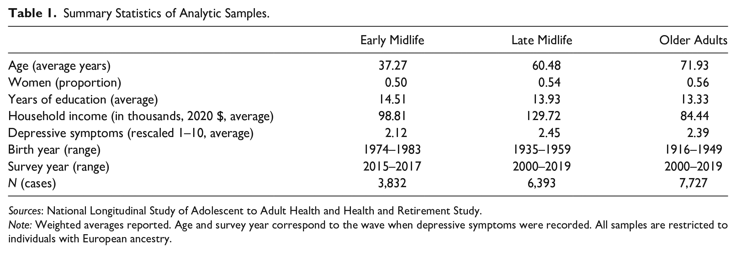
Sources: National Longitudinal Study of Adolescent to Adult Health and Health and Retirement Study.

Note: Weighted averages reported. Age and survey year correspond to the wave when depressive symptoms were recorded. All samples are restricted to individuals with European ancestry.

Depressive Symptoms

Measures of depressive symptoms (DS) are based on abbreviated versions of the Center for Epidemiologic Studies Depression (CES-D) scale (Radloff 1977). Abbreviated versions of this scale were administered in Add Health (a five-item version) and HRS (an eight-item, dichotomous-response version). These indices have been validated in prior studies and share psychometric properties with the full CES-D (Perreira et al. 2005; Turvey, Wallace, and Herzog 1999). Both indices have good internal consistency in the analytic samples (α = 0.81 in Add Health and α = 0.78 in HRS). Outcomes are standardized to create z scores comparable across samples.

Income

Both data sets reported pretax household income. In Add Health, income excludes government transfers and is measured on a categorical scale. Income was transformed into a continuous measure using midpoint approximation; for the highest income bin, income is approximated at 33 percent above the lower bound. Income in HRS includes government transfers (Bugliari et al. 2021). I bottom-coded household income at $500. Current income corresponds to Wave 5 in Add Health and the last wave in the HRS analytical sample. Permanent income in Add Health is averaged over Waves 4 and 5 (about 10 years), and in HRS, it is averaged over three consecutive waves (roughly 5 years)—this corresponds to approximations used in previous research (e.g., D’Ambrosio et al. 2020; Gangl 2005).⁶ Income measures are adjusted for inflation using implicit price deflator indexed for 2020.

The relationship between income and various indicators of mental well-being tends to follow a log-linear pattern (e.g., Stevenson and Wolfers 2013; Zimmerman and Katon 2005), indicating that the marginal effect of an absolute increase in income diminishes with the level of income. This pattern is also reflected in the samples used in this study (discussed further in the results section). As such, I use logged measures of both current and permanent income. The gradient with respect to log income reflects the average effect of a percentage change in income.

Polygenic Predictors

Most traits are understood to be polygenic, that is, affected by multiple genetic variants (McCarthy et al. 2008). To identify the causal genetic variants, GWASs are conducted in large samples, which entail estimating regressions of the trait of interest on each variant, typically a single nucleotide polymorphism (SNP; for a succinct primer, see Conley 2016). GWASs are estimated within ancestrally homogeneous populations and control for gender, age, and principal components of genetic ancestry that adjust for population stratification within ancestral groups.⁷ The GWAS yields summary statistics, comprising of a separate regression coefficient for each SNP, which are used as weights to construct polygenic indices (PGIs), as follows:

P G I_{i} = \sum_{j = 1}^{k} β_{j} S N P_{i j}

where i indexes individuals and j indexes the frequency of the less frequent (“minor”) allele on the jth SNP. β_j is the coefficient of the effect of $S N P_{j}$ on the trait. To avoid overfitting, the sample for which a PGI is constructed is not part of the data set on which the GWAS is based. The PGIs are standardized to have mean of 0 and variance of 1 within each sample.

PGIs used in this study are derived from analyses by Becker et al. (2021). These PGIs are based on multitrait analysis of GWAS, which leverages shared genetic variance between phenotypes to enhance the predictive power of any given PGI (Turley et al. 2018). I use a PGI of DS as a genetic control and a PGI of educational attainment (EA) as an instrument for income. The EA-PGI can affect income through a number of socially mediated pathways, including, most directly, via educational attainment and through potential indirect pathways, including occupational aspirations, financial savvy, and selection of a spouse with high socioeconomic status (SES; Barban et al. 2021; Barth, Papageorge, and Thom 2019; Belsky et al. 2016, 2018). Assumptions entailed in using the PGI as an instrumental variable are discussed in the following section.

Analytic Strategy

The analytic strategy is twofold. First, I estimate the baseline OLS, which is consistent with previous associational studies (Model 1). I then make two adjustments to the baseline model. In Model 2, I use permanent instead of current income to assess the extent of attenuation bias induced by noise in income measurement. Model 3 includes a control for the depression-PGI, which will help assess the extent to which reverse causation (attributable to genetic risk of depression) is responsible for inflating the income-depression gradient. The OLS models are specified as follows:

D S_{i} = β_{O L S} . I n c o m e_{i} + X_{i} δ + ε_{i}

(1)

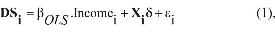
where i indexes individuals, X is a vector of covariates, and the coefficient β estimates the income effect conditional on X. The standard set of covariates across models includes the first 10 principal components of genetic ancestry, gender, and age (Burgess et al. 2019). HRS analyses also include period fixed effects to adjust for variation in timing of data collection. For reasons discussed earlier, I do not control for variables that could be affected by income (e.g., health or marital status).

It should be noted that estimates of the income coefficient in Model 3 may be upwardly biased due to classical measurement error in the depression-PGI, which gets incorporated in the computation of PGIs from GWAS summary statistics (Becker et al. 2021). In turn, this noise can attenuate the coefficient of the PGI and inflate that of income. Ancillary analyses tested the sensitivity of these models to measurement error and are discussed later.

While the aformentioned models address biases due to measurement error and reverse causation, they do not address omitted variable bias. As mentioned earlier, controlling for omitted variables in this case is complicated by the fact that some key sources of confounding (e.g., marital status and health) also mediate the effects of income on mental health. As such, a different strategy is needed to assess the effects of income differences between individuals. I use two-stage least squares (2SLS) regressions to estimate this effect (Wooldridge 2010). In the first-stage equation, I use the EA-PGI as an instrumental variable for income to predict the proportion of income that, net of covariates, is not caused by factors that confound the income-depression relationship. The predicted values of income from this model are then used to estimate the income effect in the second stage. The 2SLS model is specified as follows:

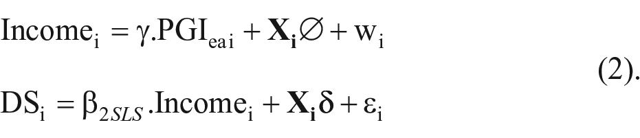
\begin{array}{l} I n c o m e_{i} = γ . P G I_{e a}_{i} + X_{i} \emptyset + w_{i} \\ D S_{i} = β_{2 S L S} . \hat{I n c o m e_{i}} + X_{i} δ + ε_{i} \end{array}

(2)

These regressions are estimated using the ivreg2 program in Stata (Baum, Schaffer, and Stillman 2010).

Two important assumptions are built into the baseline 2SLS model. First, the EA-PGI needs to be a significant and strong predictor of income. The violation of this assumption can result in “weak instrument bias,” which could exaggerate $β_{2 S L S}$ estimates (Staiger and Stock 1997). As such, I first test that the instrument is relevant and strong by comparing F statistics from the first-stage regression with critical values from the Stock-Yogo test for a true rejection rate of 5 percent and a maximum tolerated rejection rate of 10 percent (Stock and Yogo 2005).

The second assumption is that there is no path from the EA-PGI to DS that is unmediated by income, also known as the “exclusion restriction” (Wooldridge 2010:91–92). It follows from this assumption that conditional on income and covariates, the EA-PGI should be randomly distributed with respect to DS. One potential source of violation of this condition is “horizontal pleiotropy,” which is induced when the same parts of the genome predict both the outcome and explanatory variable (Paaby and Rockman 2013). Indeed, the PGIs of EA and depression are significantly negatively correlated in these estimation samples (in Add Health, ρ = −.35, p < .001; in HRS, ρ = −.29, p < .001). To address this, I estimate an adjusted 2SLS model controlling for the depression-PGI (DiPrete et al. 2018).⁸ A second source of violation is “genetic nurture”—that is, the indirect influence of parents’ genes on a person’s mental well-being that is transmitted via the rearing environment (Kong et al. 2018)—which can induce a correlation between EA-PGI and depression. This concern is partly mitigated by controlling for parental education (Hart, Little, and van Bergen 2021).^9,10 Sample sizes for the adjusted 2SLS models are relatively smaller due to missing parental education data.

Another assumption about the exclusion restriction is that education and depressive symptoms are conditionally independent. This assumption is supported by previous causal research (Avendano, de Coulon, and Nafilyan 2020; Dahmann and Schnitzlein 2019; Sperandei et al. 2023). However, in ancillary analyses, I also test this assumption by decomposing the causal education effect into income and nonincome effects (Dippel et al. 2020). While this decomposition method itself entails assumptions that may not be fully satisfied, it provides at least some useful benchmarks for the extent and direction of bias in $β_{2 S L S}$ induced by a nonincome effect of education. Supplement C provides full details of the method and analysis, and the results of the 2SLS models are discussed in light of the decomposition analysis.

Results

Using Permanent Income Instead of Current Income

I begin by discussing patterns of association between DS and logged income measures. Figure 1 depicts the income-depression gradient with respect to log of current and permanent income in the three samples. Consistent with expectations based on prior research, the gradient with respect to permanent income is steeper across all three samples.

Figure 1.

Relationship between depressive symptoms and income.

Results of OLS models are summarized in Figure 2. In the baseline OLS model, current income gradients range between −.2 and −.3 (full results in Table S1).¹¹ The gradients with respect to permanent income are larger, by .05 SD on average, suggesting that fluctuations or measurement errors in current income are a potential source of attenuation bias. For both current and permanent income, coefficient estimates for older adults are significantly smaller compared to estimates for adults in early and late midlife.

Figure 2.

Ordinary least squares estimates of the income-depression gradient across adult life stages.

Adjusting for Genetic Risk of Depression

Across all three age groups, average DS between individuals significantly vary by the depression-PGI (Figure 3). This variation in mental health is reflecting influences that rather than being caused by income, may conversely influence income attainment. Indeed, when a control for the depression-PGI is included in Model 3, estimates of the standard OLS model shrink by about .01 SD (Figure 2 and Table S1). As mentioned earlier, these analyses may underestimate reverse causation due to measurement error in the DS-PGI (Becker et al. 2021). In ancillary analyses, estimates adjusted for measurement error contract the estimates of income effect by.02 SD on average (Table S6). Again, estimates for older adulthood are substantially smaller compared to earlier in the life course.

Figure 3.

Distribution of depressive symptoms by depression PGI.

Two-Stage Least Squares Estimation of Causal Income Effect

The 2SLS models assess the extent of bias in the income-depression gradient resulting from factors in addition to those discussed previously. The first-stage regression predicts the proportion of income that is in turn predicted by the EA-PGI. Income differences between individuals significantly vary by the EA-PGI across all three samples in both the baseline models and models adjusted for depression-PGI and parental SES (left panel in Figure 4). Across all first-stage models, the EA-PGI has a significant coefficient, and the first-stage F statistics are larger than critical value of 16.38 (Stock and Yogo 2005), indicating that the instrument relevance condition is satisfied (Table S2).¹²

Figure 4.

Two-stage least squares estimates of income effect on depressive symptoms.

All estimates from the baseline 2SLS models are statistically significant (right panel in Figure 4 and Table S3) and are comparable in magnitude to the gradient estimated from OLS regressions. Because the confidence intervals of 2SLS estimates are wider, differences between estimates for late midlife and older adulthood are no longer distinguishable, but early midlife estimates are significantly smaller than estimates for older adulthood. As discussed earlier, baseline estimates could be biased due to horizontal pleiotropy and genetic nurture. The adjusted 2SLS model assesses the sensitivity of estimates to these biases. In the adjusted model, estimates remain significant for older adulthood and are marginally significant for late midlife (p = .06) but are insignificant for early midlife. In terms of magnitude, the adjusted 2SLS estimates for the two older age groups are comparable to OLS coefficients, but estimates for early midlife are virtually zero. The consistency of estimates across baseline and adjusted models suggests that income does have a causal effect on depression in late midlife and older adulthood.

The 2SLS models also assume that net of income, education does not directly affect DS. To assess how much the violation of this assumption might bias 2SLS estimates, I conducted a decomposition analysis assessing the effect of education on DS via income and nonincome pathways (Figure 5 and Table S4). In the baseline models, the total effect of education is negative, with nearly all of the beneficial effect being driven via the income effect; the nonincome effect is positive. In the adjusted models, this pattern continues to hold for late midlife and older adulthood (suggesting that the assumption of a negligible nonincome effect of the EA-PGI is largely valid and results in only a small amount of downward bias in the 2SLS estimates). However, income effect is reversed in the early midlife sample when additional covariates are included, indicating that the exclusion restriction is strongly violated for this sample. Ancillary analyses show that the direction of income effect in early midlife specifically flips when parental education is included in the model. A potential reason may be that parental SES is more strongly correlated with household income in early midlife than at later ages (e.g., in Wave 5, about 8 percent of Add Health participants lived with their parents, and 11 percent received large financial transfers from parents and other relatives).

Figure 5.

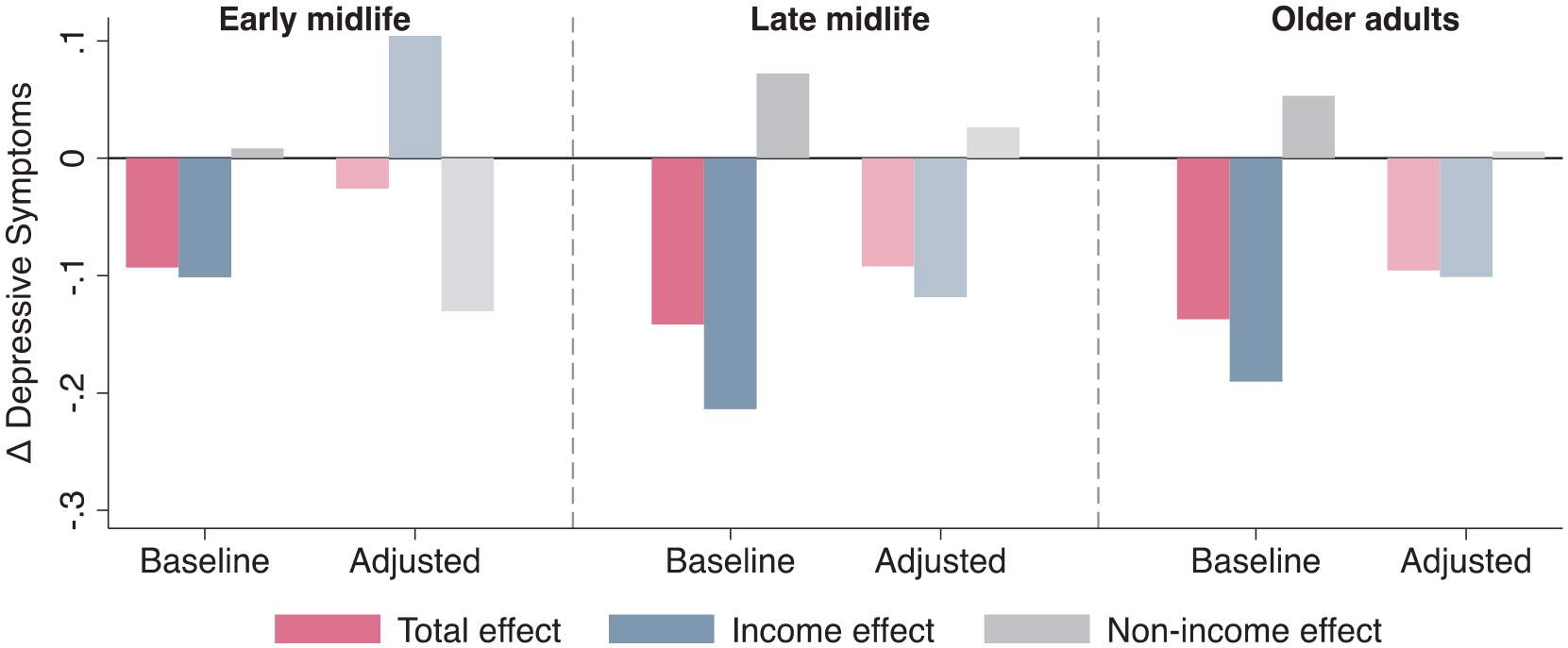
Decomposition of effect of education on depressive symptoms.

A final concern is that the EA-PGI only captures income variation via pathways affected by the PGI. Income can of course also vary due to other reasons, and in turn, these alternative pathways to a higher income can have distinct implications for mental well-being. More generally, the concern is that 2SLS estimates reflect local average treatment effects based on “compliers,” who may differ from the sample average (Card 2001; Imbens and Angrist 1994). Ancillary analyses approximating the profile of compliers (using an approach outlined by Marbach and Hangartner 2020) indicate that compliers were largely similar to the full sample in terms of class background, gender, birth cohort, and depression PGI (Figures S1–S3).

Discussion

Social scientists have long documented a negative gradient between income and mental health, but whether this correlation reflects a causal effect has been an open question. Indeed, several previous causal studies have reported small, null, and even negative mental health effects. This study assessed this problem from a different vantage using data and methods different from those employed in previous literature. Results suggested that measurement errors in income and reverse causation due to the genetic risk of depression are meaningful sources of bias, acting in opposite directions. In models estimating putatively causal effects of income, the effect sizes were as large as the income-depression gradient for adults age 50 and older. For the early midlife sample, the more stringent assumptions of the causal model were not satisfied, but estimates from the less stringent model aligned with those for older adults. Age differences in estimates—while present—were relatively small and inconsistent in direction across OLS and 2SLS regressions.

Key limitations of these analyses include the following. Because genetic data are not representative of underlying populations at all levels of data collection, we cannot directly use PGIs derived from European ancestry populations in non-European ancestry samples with reasonable confidence. While using permanent income is an improvement over prior literature, these estimates are averaged across heterogeneous adult income trajectories (Frech and Damaske 2019; Song et al. 2022), which is a residual source of noise. A shortcoming shared with prior literature is that the income measures are not fully adjusted for fiscal transfers. Fiscally adjusted income distributions tend to be less unequal (Brady et al. 2018), which could have implications for these results. Finally, the exclusion restriction for the 2SLS estimator was not fully satisfied across samples, being strongly violated in the early midlife sample.

This article makes two contributions to the understanding of the income-depression link. First, improvements to the associational model allow adjudging the extent to which two major known sources of bias might be affecting estimates of the income–well-being gradient. The fact that this gradient only marginally changed due to these corrections—and the biases acted in opposite directions—suggests that these are perhaps not the most worrisome sources of bias. Second, the putative causal effect of income was estimated using an approach that—while not free of limitations—does not suffer from the same shortcomings as previous causal designs. Specifically, it was an improvement over previous studies using natural experiments or policy changes that typically capture short-term and narrow effects of income shocks and family studies where within-family effects do not readily generalize to unrelated individuals. Pooled across samples and models, the results presented here are suggestive of an average beneficial causal effect of income on mental well-being.

Supplemental Material

sj-pdf-1-srd-10.1177_23780231231186072 – Supplemental material for Mental Health Effects of Income over the Adult Life Course

Supplemental material, sj-pdf-1-srd-10.1177_23780231231186072 for Mental Health Effects of Income over the Adult Life Course by Tamkinat Rauf in Socius

Footnotes

Authors’ Note

Replication files are available at https://osf.io/grjs9/. Add Health restricted-use data can be requested at: https://data.cpc.unc.edu/projects/2/view. HRS data are publicly-accessible at: .

Funding

The author(s) disclosed receipt of the following financial support for the research, authorship, and/or publication of this article: The article uses data from the Health and Retirement Study, which is conducted by the University of Michigan and is sponsored by the National Institute on Aging (NIA U01AG009740), and the National Longitudinal Study of Adolescent to Adult Health, which is conducted by the University of North Carolina at Chapel Hill and is sponsored by the National Institute on Aging (NIA U01AG071448 and U01AG071450). This research was supported by the Stanford Sociology Research Opportunity Grant and a dissertation fellowship by the Stanford Institute for Research in the Social Sciences.

ORCID iD

Tamkinat Rauf

Supplemental Material

Supplemental material for this article is available online.

Notes

Author Biography

Tamkinat Rauf is a post-doctoral fellow and an incoming assistant professor in the Department of Sociology at the University of Wisconsin-Madison. Her research examines how social, economic, political, and biological factors jointly influence various aspects of human well-being, including mental and physical health.

References

Alderson

Arthur S.

Katz-Gerro

Tally

. 2016. “Compared to Whom? Inequality, Social Comparison, and Happiness in the United States.” Social Forces 95(1):25–54.

Angrist

Joshua

Pischke

Jörn-Steffen

. 2008. Mostly Harmless Econometrics: An Empiricist’s Companion. Princeton, NJ: Princeton University Press.

Apouey

Benedicte

Clark

Andrew E.

2015. “Winning Big but Feeling No Better? The Effect of Lottery Prizes on Physical and Mental Health.” Health Economics 24(5):516–38.

Arnett

Jeffrey Jensen

. 2012. “New Horizons in Research on Emerging and Young Adulthood.” Pp. 231–44 in Early Adulthood in a Family Context, edited by Booth

Brown

S. L.

Landale

N. S.

Manning

W. D.

McHale

S. M.

New York, NY: Springer.

Avendano

Mauricio

de Coulon

Augustin

Nafilyan

Vahé

. 2020. “Does Longer Compulsory Schooling Affect Mental Health? Evidence from a British Reform.” Journal of Public Economics 183:104137. doi:10.1016/j.jpubeco.2020.104137.

Barban

Nicola

De Cao

Elisabetta

Oreffice

Sonia

Quintana-Domeque

Climent

. 2021. “The Effect of Education on Spousal Education: A Genetic Approach.” Labour Economics 71:102023. doi:10.1016/j.labeco.2021.102023.

Barcellos

Silvia H.

Carvalho

Leandro

Turley

Patrick

. 2021. “The Effect of Education on the Relationship between Genetics, Early-Life Disadvantages, and Later-Life SES.” NBER Working Paper No. 28750, National Bureau of Economic Research. http://www.nber.org/papers/w28750.

Bartels

Meike

. 2015. “Genetics of Wellbeing and Its Components Satisfaction with Life, Happiness, and Quality of Life: A Review and Meta-analysis of Heritability Studies.” Behavior Genetics 45:137–56.

Barth

Daniel

Papageorge

Nicholas W.

Thom

Kevin

. 2019. “Genetic Endowments and Wealth Inequality.” Journal of Political Economy 128(4):1474–522.

10.

Baum

Christopher F.

Schaffer

Mark E.

Stillman

Steven

. 2010. “ivreg2: Stata Module for Extended Instrumental Variables/2SLS, GMM and AC/HAC, LIML and k-Class Regression.” http://ideas.repec.org/c/boc/bocode/s425401.html.

11.

Bayer

Christian

Juessen

Falko

. 2015. “Happiness and the Persistence of Income Shocks.” American Economic Journal: Macroeconomics 7(4):160–87.

12.

Becker

Joel

Burik

Casper A. P.

Goldman

Grant

Wang

Nancy

Jayashankar

Hariharan

Bennett

Michael

Belsky

Daniel W.

, et al. 2021. “Resource Profile and User Guide of the Polygenic Index Repository.” Nature Human Behaviour 5(12):1744–58.

13.

Belsky

Daniel W.

Domingue

Benjamin W.

Wedow

Robbee

Arseneault

Louise

Boardman

Jason D.

Caspi

Avshalom

Conley

Dalton

, et al. 2018. “Genetic Analysis of Social-Class Mobility in Five Longitudinal Studies.” Proceedings of the National Academy of Sciences 115(31):E7275–84.

14.

Belsky

Daniel W.

Moffitt

Terrie E.

Corcoran

David L.

Domingue

Benjamin

Harrington

Hona Lee

Hogan

Sean

Houts

Renate

, et al. 2016. “The Genetics of Success: How Single-Nucleotide Polymorphisms Associated with Educational Attainment Relate to Life-Course Development.” Psychological Science 27(7):957–72.

15.

Berkessel

Jana B.

Gebauer

Jochen E.

Joshanloo

Mohsen

Bleidorn

Wiebke

Rentfrow

Peter J.

Potter

Jeff

Gosling

Samuel D.

2021. “National Religiosity Eases the Psychological Burden of Poverty.” Proceedings of the National Academy of Sciences of the United States of America 118(39):1–6.

16.

Boertien

Diederik

. 2012. “Jackpot? Gender Differences in the Effects of Lottery Wins on Separation.” Journal of Marriage and Family 74(5):1038–53.

17.

Bollen

Kenneth A.

2012. “Instrumental Variables in Sociology and the Social Sciences.” Annual Review of Sociology 38:37–72.

18.

Bourdieu

Pierre

. 1979. Distinction: A Social Critique of the Judgement of Taste. London: Routledge.

19.

Boyd-Swan

Casey

Herbst

Chris M.

Ifcher

John

Zarghamee

Homa

. 2016. “The Earned Income Tax Credit, Mental Health, and Happiness.” Journal of Economic Behavior and Organization 126:18–38.

20.

Brady

David

Giesselmann

Marco

Kohler

Ulrich

Radenacker

Anke

. 2018. “How to Measure and Proxy Permanent Income: Evidence from Germany and the U.S.” Journal of Economic Inequality 16(3):321–45.

21.

Brickman

Philip

Coates

Dan

Janoff-Bulman

Ronnie

. 1978. “Lottery Winners and Accident Victims: Is Happiness Relative?” Journal of Personality and Social Psychology 36(8):917–27.

22.

Bugliari

Delia

Carroll

Joanna

Hayden

Orla

Hayes

Jessica

Hurd

Michael

Karabatakis

Adam

Main

Regan

, et al. 2021. “RAND HRS Longitudinal File 2018 (V2) Documentation (Final Release). RAND Corporation, Santa Monica, CA.”

23.

Burgess

Stephen

Smith

George Davey

Davies

Neil M.

Dudbridge

Frank

Gill

Dipender

Glymour

M. Maria

Hartwig

Fernando P.

, et al. 2019. “Guidelines for Performing Mendelian Randomization Investigations.” Wellcome Open Research 4(186):1–19.

24.

Businelle

Michael S.

Mills

Britain A.

Chartier

Karen G.

Kendzor

Darla E.

Reingle

Jennifer M.

Shuval

Kerem

. 2014. “Do Stressful Events Account for the Link between Socioeconomic Status and Mental Health?” Journal of Public Health 36(2):205–12.

25.

Card

David

. 2001. “Estimating the Return to Schooling: Progress on Some Persistent Econometric Problems.” Econometrica 69(5):1127–60.

26.

Case

Anne

Fertig

Angela

Paxson

Christina

. 2005. “The Lasting Impact of Childhood Health and Circumstance.” Journal of Health Economics 24(2):365–89.

27.

Cesarini

David

Lindqvist

Erik

Ostling

Robert

Wallace

Bjorn

. 2016. “Wealth, Health, and Child Development: Evidence from Administrative Data on Swedish Lottery Players.” The Quarterly Journal of Economics 131(2):687–738.

28.

Cherlin

Andrew J.

2010. “Demographic Trends in the United States: A Review of Research in the 2000s.” Journal of Marriage and Family 72(3):403–19.

29.

Chetty

Raj

Stepner

Michael

Abraham

Sarah

Lin

Shelby

Scuderi

Benjamin

Turner

Nicholas

Bergeron

Augustin

, et al. 2016. “The Association between Income and Life Expectancy in the United States, 2001-2014.” Journal of the American Medical Association 315(16):1750–66.

30.

Cheung

Felix

Lucas

Richard E.

2015. “When Does Money Matter Most? Examining the Association between Income and Life Satisfaction over the Life Course.” Psychology and Aging 30(1):120–35.

31.

Conley

Dalton

. 2016. “Socio-genomic Research Using Genome-Wide Molecular Data.” Annual Review of Sociology 42(1):275–99.

32.

Courtin

Emilie

Muennig

Peter

Verma

Nandita

Riccio

James A.

Lagarde

Mylene

Vineis

Paolo

Kawachi

Ichiro

, et al. 2018. “Conditional Cash Transfers and Health of Low-Income Families in the US: Evaluating the Family Rewards Experiment.” Health Affairs 37(3):438–46.

33.

Dahmann

Sarah C.

Schnitzlein

Daniel D.

2019. “No Evidence for a Protective Effect of Education on Mental Health.” Social Science and Medicine 241:112584. doi:10.1016/j.socscimed.2019.112584.

34.

D’Ambrosio

Conchita

Jäntti

Markus

Lepinteur

Anthony

. 2020. “Money and Happiness: Income, Wealth and Subjective Well-Being.” Social Indicators Research 148(1):47–66.

35.

Smith

Davey

George Ebrahim

Shah

. 2003. “‘Mendelian Randomization’: Can Genetic Epidemiology Contribute to Understanding Environmental Determinants of Disease?” International Journal of Epidemiology 32(1):1–22.

36.

De Neve

Jan Emmanuel

Oswald

Andrew J.

2012. “Estimating the Influence of Life Satisfaction and Positive Affect on Later Income Using Sibling Fixed Effects.” Proceedings of the National Academy of Sciences of the United States of America 109(49):19953–58.

37.

Diebold

Francis X.

Rudebusch

Glenn D.

1991. “Is Consumption Too Smooth? Long Memory and the Deaton Paradox.” The Review of Economics and Statistics 73(1):1–9.

38.

Dippel

Christian

Gold

Robert

Heblich

Stephan

Pinto

Rodrigo

. 2020. “Mediation Analysis in IV Settings with a Single Instrument.” https://christiandippel.com/IVmediate_.pdf.

39.

DiPrete

Thomas A.

Burik

Casper A. P.

Koellinger

Philipp D.

2018. “Genetic Instrumental Variable Regression: Explaining Socioeconomic and Health Outcomes in Nonexperimental Data.” Proceedings of the National Academy of Sciences of the United States of America 115(22):E4970–79.

40.

Dooley

David

Prause

Joann

Ham-Rowbottom

Kathleen

. 2000. “Underemployment and Depression: Longitudinal Relationships.” Journal of Health and Social Behavior 41(4):421–36.

41.

Eaton

William W.

Muntaner

Carles

Bovasso

Gregory

Smith

Corey

. 2001. “Socioeconomic Status and Depressive Syndrome: The Role of Inter- and Intra-generational Mobility, Government Assistance, and Work Environment.” Journal of Health and Social Behavior 42(3):277–94.

42.

Elder

Glen H.

1994. “Time, Human Agency, and Social Change: Perspectives on the Life Course.” Social Psychology Quarterly 57(1):4–15.

43.

Elder

Glen H.

1998. “The Life Course as Developmental Theory.” Child Development 69(1):1–12.

44.

Ellison

Christopher G.

1991. “Religious Involvement and Subjective Well-Being.” Journal of Health and Social Behavior 32(1):80–99.

45.

Erikson

Erik H.

1968. Identity: Youth and Crisis. New York, NY: W. W. Norton & Company.

46.

Fletcher

Jason

. 2013. “Adolescent Depression and Adult Labor Market Outcomes.” Southern Economic Journal 80(1):26–49.

47.

Frech

Adrianne

Damaske

Sarah

. 2019. “Men’s Income Trajectories and Physical and Mental Health at Midlife.” American Journal of Sociology 124(5):1372–412.

48.

Freese

Jeremy

. 2008. “Genetics and the Social Science Explanation of Individual Outcomes.” American Journal of Sociology 114(Suppl.):S1–35.

49.

Freese

Jeremy

. 2017. “What about the Behavioral Constellation of Advantage?” Behavioral and Brain Sciences 40:e326. doi:10.1017/S0140525X17000966.

50.

Freese

Jeremy

. 2018. “The Arrival of Social Science Genomics.” Contemporary Sociology 47(5):524–36.

51.

Gangl

Markus

. 2005. “Income Inequality, Permanent Incomes, and Income Dynamics: Comparing Europe to the United States.” Work and Occupations 32(2):140–62.

52.

Gardner

Jonathan

Oswald

Andrew J.

2007. “Money and Mental Wellbeing: A Longitudinal Study of Medium-Sized Lottery Wins.” Journal of Health Economics 26(1):49–60.

53.

Golberstein

Ezra

. 2015. “The Effects of Income on Mental Health: Evidence from the Social Security Notch.” The Journal of Mental Health Policy and Economics 18(1):27–37.

54.

Griliches

Zvi

. 1977. “Estimating the Returns to Schooling: Some Econometric Problems.” Econometrica 45(1):1–22.

55.

Gundlach

Erich

Opfinger

Matthias

. 2013. “Religiosity as a Determinant of Happiness.” Review of Development Economics 17(3):523–39.

56.

Haas

Steven A.

2006. “Health Selection and the Process of Social Stratification: The Effect of Childhood Health on Socioeconomic Attainment.” Journal of Health and Social Behavior 47(4):339–54.

57.

Hanandita

Wulung

Tampubolon

Gindo

. 2014. “Does Poverty Reduce Mental Health? An Instrumental Variable Analysis.” Social Science and Medicine 113:59–67.

58.

Hankins

Scott

Hoekstra

Mark

. 2011. “Lucky in Life, Unlucky in Love?: The Effect of Random Income Shocks on Marriage and Divorce.” Journal of Human Resources 46(2):403–26.

59.

Harris

Kathleen Mullan

Udry

J. Richard

. 2018. “The National Longitudinal Study of Adolescent to Adult Health (Add Health), Waves I-V” [Machine-readable data file and documentation]. Chapel Hill: Carolina Population Center, University of North Carolina.

60.

Hart

Sara A.

Little

Callie

van Bergen

Elsje

. 2021. “Nurture Might Be Nature: Cautionary Tales and Proposed Solutions.” Nature Science of Learning 6(1):1–12.

61.

Hastings

Orestes P.

Roeser

Kassandra K.

2020. “Happiness in Hard Times: Does Religion Buffer the Negative Effect of Unemployment on Happiness?” Social Forces 99(2):447–73.

62.

Health and Retirement Study. 2021. “Health and Retirement Study, Public Use Dataset.” https://hrs.isr.umich.edu/data-products.

63.

Heflin

Colleen M.

Iceland

John

. 2009. “Poverty, Material Hardship, and Depression.” Social Science Quarterly 90(5):1051–71.

64.

Hendren

Nathaniel

. 2017. “Knowledge of Future Job Loss and Implications for Unemployment Insurance.” American Economic Review 107(7):1778–823.

65.

Herzer

Dierk

Strulik

Holger

. 2017. “Religiosity and Income: A Panel Cointegration and Causality Analysis.” Applied Economics 49(30):2922–38.

66.

Howard

David M.

Adams

Mark J.

Clarke

Toni Kim

Hafferty

Jonathan D.

Gibson

Jude

Shirali

Masoud

Coleman

Jonathan R. I.

, et al. 2019. “Genome-Wide Meta-analysis of Depression Identifies 102 Independent Variants and Highlights the Importance of the Prefrontal Brain Regions.” Nature Neuroscience 22(3):343–52.

67.

Hughes

Amanda

Wade

Kaitlin H.

Dickson

Matt

Rice

Frances

Davies

Alisha

Davies

Neil M.

Howe

Laura D.

2021. “Common Health Conditions in Childhood and Adolescence, School Absence, and Educational Attainment: Mendelian Randomization Study.” NPJ Science of Learning 6(1):1–9.

68.

Huguet

Pascal

Carlier

Michèle

Dolan

Conor V.

De Geus

Eco J.

Boomsma

Dorret I.

2017. “Social Comparison Orientation in Monozygotic and Dizygotic Twins.” Twin Research and Human Genetics 20(6):550–57.

69.

Imbens

Guido W.

Angrist

Joshua D.

1994. “Identification and Estimation of Local Average Treatment Effects.” Econometrica 62(2):467–75.

70.

Jacob

Marita

Kleinert

Corinna

. 2014. “Marriage, Gender, and Class: The Effects of Partner Resources on Unemployment Exit in Germany.” Social Forces 92(3):839–71.

71.

Jaroszewicz

Ania

Jachimowicz

Jon M.

Hauser

Oliver P.

Jamison

Julian

. 2022. “How Effective Is (More) Money? Randomizing Unconditional Cash Transfer Amounts in the US.” SSRN. https://papers.ssrn.com/sol3/papers.cfm?abstract_id=4154000.

72.

Karney

Benjamin R.

2021. “Socioeconomic Status and Intimate Relationships.” Annual Review of Psychology 72:2.1–2.4.

73.

Kessler

Ronald C.

1982. “A Disaggregation of the Relationship between Socioeconomic Status and Psychological Distress.” American Sociological Review 47(6):752–64.

74.

Killewald

Alexandra

Lundberg

Ian

. 2017. “New Evidence against a Causal Marriage Wage Premium.” Demography 54(3):1007–28.

75.

King

Katherine

Ogle

Christin

. 2014. “Negative Life Events Vary by Neighborhood and Mediate the Relation between Neighborhood Context and Psychological Well-Being.” PLoS One 9(4):e93539. doi:10.1371/journal.pone.0093539.

76.

Kong

Augustine

Thorleifsson

Gudmar

Frigge

Michael L.

Vilhjalmsson

Bjarni J.

Young

Alexander I.

Thorgeirsson

Thorgeir E.

Benonisdottir

Stefania

, et al. 2018. “The Nature of Nurture: Effects of Parental Genotypes.” Science 359(6374):424–28.

77.

Kraus

Michael W.

Piff

Paul K.

Keltner

Dacher

. 2009. “Social Class, Sense of Control, and Social Explanation.” Journal of Personality and Social Psychology 97(6):992–1004.

78.

Lam

Janine R.

Tyler

Jessica

Scurrah

Katrina J.

Reavley

Nicola J.

Dite

Gillian S.

2019. “The Association between Socioeconomic Status and Psychological Distress: A within and between Twin Study.” Twin Research and Human Genetics 22(5):312–20.

79.

Levitt

Steven D.

1999. “The Changing Relationship between Income and Crime Victimization.” Economic Policy Review 5(3):87–98.

80.

Hongbin

Liu

Pak Wai

Maoliang

Zhang

Junsen

. 2014. “Does Money Buy Happiness? Evidence from Twins in Urban China.” https://www.semanticscholar.org/paper/Does-Money-Buy-Happiness-Evidence-from-Twins-in-Li-Liu/98f621335d9b48f227daa41cbc4d21d355300716

81.

Liao

Tim Futing

. 2021. “Income Inequality, Social Comparison, and Happiness in the United States.” Socius 7. doi:10.1177/2378023120985648.

82.

Lim

Kai Xiang

Rijsdijk

Frühling

Hagenaars

Saskia P.

Socrates

Adam

Choi

Shing Wan

Coleman

Jonathan R. I.

Glanville

Kylie P.

, et al. 2020. “Studying Individual Risk Factors for Self-Harm in the UK Biobank: A Polygenic Scoring and Mendelian Randomisation Study.” PLoS Medicine 17(6):e1003137. doi:10.1371/journal.pmed.1003137.

83.

Lindqvist

Erik

Östling

Robert

Cesarini

David

. 2020. “Long-Run Effects of Lottery Wealth on Psychological Well-Being.” Review of Economic Studies 87(6):2703–26.

84.

Ludwig

Volker

Brüderl

Josef

. 2018. “Is There a Male Marital Wage Premium? New Evidence from the United States.” American Sociological Review 83(4):744–70.

85.

Luhmann

Maike

Schimmack

Ulrich

Eid

Michael

. 2011. “Stability and Variability in the Relationship between Subjective Well-Being and Income.” Journal of Research in Personality 45(2):186–97.

86.

Luo

Waite

Linda J.

2005. “The Impact of Childhood and Adult SES on Physical, Mental, and Cognitive Well-Being in Later Life.” The Journals of Gerontology. Series B, Psychological Sciences and Social Sciences 60(2):S93–101.

87.

Marbach

Moritz

Hangartner

Dominik

. 2020. “Profiling Compliers and Noncompliers for Instrumental-Variable Analysis.” Political Analysis 28(3):435–44.

88.

Marmot

Michael

. 2002. “The Influence of Income on Health: Views of an Epidemiologist.” Health Affairs 21(2):31–46.

89.

Martikainen

Pekka

Adda

Jerome

Ferrie

Jane E.

Smith

George Davey

Marmot

Michael

. 2003. “Effects of Income and Wealth on GHQ Depression and Poor Self Rated Health in White Collar Women and Men in the Whitehall II Study.” Journal of Epidemiology and Community Health 57(9):718–23.

90.

Martin

Alicia R.

Kanai

Masahiro

Kamatani

Yoichiro

Okada

Yukinori

Neale

Benjamin M.

Daly

Mark J.

2019. “Clinical Use of Current Polygenic Risk Scores May Exacerbate Health Disparities.” Nature Genetics 51(4):584–91.

91.

McCarthy

Mark I.

Abecasis

Gonçalo R.

Cardon

Lon R.

Goldstein

David B.

Little

Julian

Ioannidis

John P. A.

Hirschhorn

Joel N.

2008. “Genome-Wide Association Studies for Complex Traits: Consensus, Uncertainty and Challenges.” Nature Reviews Genetics 9(5):356–69.

92.

McGarry

Kathleen

. 2016. “Dynamic Aspects of Family Transfers.” Journal of Public Economics 137:1–13.

93.

McLeod

Jane D.

2013. “Social Stratification and Inequality.” Pp. 229–53 in Handbook of the Sociology of Mental Health, edited by Aneshensel

C. S.

Phelan

J. C.

Dordrecht

A. Bierman.

Netherlands: Springer.

94.

McLeod

Jane D.

Kessler

Ronald C.

1990. “Socioeconomic Status Differences in Vulnerability to Undesirable Life Events.” Journal of Health and Social Behavior 31(2):162–72.

95.

Miech

Richard Allen

Shanahan

Michael J.

2000. “Socioeconomic Status and Depression over the Life Course.” Journal of Health and Social Behavior 41(2):162–76.

96.

Muntaner

Carles

Borrell

Carme

Chung

Haejoo

. 2007. “Class Relations, Economic Inequality and Mental Health: Why Social Class Matters to the Sociology of Mental Health.” Pp. 127–41 in Mental Health, Social Mirror, edited by Avison

W. R.

McLeod

J. D.

Pescosolido

B. A.

Boston, MA: Springer.

97.

Oswald

Andrew J.

Proto

Eugenio

Sgroi

Daniel

. 2015. “Happiness and Productivity.” Journal of Labor Economics 33(4):789–822.

98.

Paaby

Annalise B.

Rockman

Matthew V.

2013. “The Many Faces of Pleiotropy.” Trends in Genetics 29(2):66–73.

99.

Park

Lora E.

Ward

Deborah E.

Naragon-Gainey

Kristin

. 2017. “It’s All about the Money (for Some): Consequences of Financially Contingent Self-Worth.” Personality and Social Psychology Bulletin 43(5):601–22.

100.

Patel

Vikram

Burns

Jonathan K.

Dhingra

Monisha

Tarver

Leslie

Kohrt

Brandon A.

Lund

Crick

. 2018. “Income Inequality and Depression: A Systematic Review and Meta-analysis of the Association and a Scoping Review of Mechanisms.” World Psychiatry 17(1):76–89.

101.

Perreira

Krista M.

Deeb-Sossa

Natalia

Harris

Kathleen Mullan

Harris

Kathleen Mullan

. 2005. “What Are We Measuring ? An Evaluation of the CES-D Across Race / Ethnicity and Immigrant Generation.” Social Forces 83(4):1567–601.

102.

Piff

Paul K.

Moskowitz

Jake P.

2018. “Wealth, Poverty, and Happiness: Social Class Is Differentially Associated with Positive Emotions.” Emotion 18(6):902–905.

103.

Plagnol

Anke C.

2011. “Financial Satisfaction over the Life Course: The Influence of Assets and Liabilities.” Journal of Economic Psychology 32(1):45–64.

104.

Powdthavee

Nattavudh

. 2010. “How Much Does Money Really Matter? Estimating the Causal Effects of Income on Happiness.” Empirical Economics 39(1):77–92.

105.

Pudrovska

Tetyana

Anikputa

Benedicta

. 2014. “Early-Life Socioeconomic Status and Mortality in Later Life: An Integration of Four Life-Course Mechanisms.” Journals of Gerontology. Series B, Psychological Sciences and Social Sciences 69(3):451–60.

106.

Radloff

Lenore S.

1977. “A Self-Report Depression Scale for Research in the General Population.” Applied Psychological Measurement 1(3):385–401.

107.

Raschke

Christian

. 2019. “Unexpected Windfalls, Education, and Mental Health: Evidence from Lottery Winners in Germany.” Applied Economics 51(2):207–18.

108.

Ridley

Matthew

Rao

Gautam

Schilbach

Frank

Patel

Vikram

. 2020. “Poverty, Depression, and Anxiety: Causal Evidence and Mechanisms.” Science 370(6522):eaay0214. doi:10.1126/science.aay0214.

109.

Ross

Catherine E.

Huber

Joan

. 1985. “Hardship and Depression.” Journal of Health and Social Behavior 26(4):312–27.

110.

Ross

Catherine E.

Mirowsky

John

. 1992. “Households, Employment, and the Sense of Control.” Social Psychology Quarterly 55(3):217–35.

111.

Sato

Kaori

Kuroda

Sachiko

Owan

Hideo

. 2020. “Mental Health Effects of Long Work Hours, Night and Weekend Work, and Short Rest Periods.” Social Science and Medicine 246:112774. doi:10.1016/j.socscimed.2019.112774.

112.

Schnittker

Jason

. 2008. “Happiness and Success: Genes, Families, and the Psychological Effects of Socioeconomic Position and Social Support.” American Journal of Sociology 114(S1):233–59.

113.

Segal

Nancy L.

1988. “Cooperation, Competition, and Altruism in Human Twinships: A Sociobiological Approach.” Pp. 168–206 in Sociobiological Perspectives on Human Development, edited by MacDonald

K. M.

New York, NY: Springer.

114.

Segal

Nancy L.

Hershberger

Scott L.

1999. “Cooperation and Competition between Twins.” Evolution and Human Behavior 20(1):29–51.

115.

Shields-Zeeman

Laura

Collin

Daniel F.

Batra

Akansha

Hamad

Rita

. 2021. “How Does Income Affect Mental Health and Health Behaviours? A Quasi-experimental Study of the Earned Income Tax Credit.” Journal of Epidemiology and Community Health 75(10):929–35.

116.

Society for Adolescent Health and Medicine. 2017. “Young Adult Health and Well-Being: A Position Statement of the Society for Adolescent Health and Medicine.” Journal of Adolescent Health 60(6):758–59.

117.

Song

Zang

Emma

Land

Kenneth C.

Zheng

Boyan

. 2022. “Intergenerational Income Mobility Table Revisited: A Trajectory Group Perspective.” Research in Social Stratification and Mobility 80:100713. doi:10.1016/j.rssm.2022.100713.

118.

Sperandei

Sandro

Page

Andrew

Spittal

Matthew J.

Pirkis

Jane

. 2023. “Low Education and Mental Health among Older Adults: The Mediating Role of Employment and Income.” Social Psychiatry and Psychiatric Epidemiology 58(5):823–31.

119.

Staiger

B. Y. Douglas

Stock

James H.

1997. “Instrumental Variables Regression with Weak Instruments.” Econometrica 65(3):557–86.

120.

Steptoe

Andrew

. 2019. “Happiness and Health.” Annual Review of Public Health 40(1):339–59.

121.

Stevenson

Betsey

Wolfers

Justin

. 2013. “Subjective Well-Being and Income: Is There Any Evidence of Satiation?” American Economic Review 103(3):598–604.

122.

Stewart-Brown

Sarah

Samaraweera

Preshila Chandimali

Taggart

Frances

Kandala

Ngianga Bakwin

Stranges

Saverio

. 2015. “Socioeconomic Gradients and Mental Health: Implications for Public Health.” British Journal of Psychiatry 206(6):461–65.

123.

Stock

James H.

Yogo

Motohiro

. 2005. “Testing for Weak Instruments in Linear IV Regression.” Pp. 80–108 in Identification and Inference for Econometric Models, edited by Andrews

D. W. K.

Stock

J. H.

Cambridge, UK: Cambridge University Press.

124.

Strully

Kate W.

2009. “Job Loss and Health in the U.S. Labor Market.” Demography 46(2):221–46.

125.

Thomson

Rachel M.

Igelström

Erik

Purba

Amrit Kaur

Shimonovich

Michal

Thomson

Hilary

McCartney

Gerry

Reeves

Aaron

, et al. 2022. “How Do Income Changes Impact on Mental Health and Wellbeing for Working-Age Adults? A Systematic Review and Meta-analysis.” The Lancet Public Health 7(6):e515–28.

126.

Trejo

Sam

Domingue

Benjamin W.

2018. “Genetic Nature or Genetic Nurture? Introducing Social Genetic Parameters to Quantify Bias in Polygenic Score Analyses.” Biodemography and Social Biology 64(3–4):187–215.

127.

Turley

Patrick

Walters

Raymond K.

Maghzian

Omeed

Okbay

Aysu

Lee

James J.

Fontana

Mark Alan

Nguyen-Viet

Tuan Anh

, et al. 2018. “Multi-trait Analysis of Genome-Wide Association Summary Statistics Using MTAG.” Nature Genetics 50(2):229–37.

128.

Turvey

Carolyn L.

Wallace

Robert B.

Herzog

Regula

. 1999. “A Revised CES-D Measure of Depressive Symptoms and a DSM-Based Measure of Major Depressive Episodes in the Elderly.” International Psychogeriatrics 11(2):139–48.

129.

Van Deurzen

Ioana

Van Ingen

Erik

Van Oorschot

Wim J. H.

2015. “Income Inequality and Depression: The Role of Social Comparisons and Coping Resources.” European Sociological Review 31(4):477–89.

130.

Wang

Jun

Chen

Qihui

Chen

Gang

Yingxiang

Kong

Guoshu

Zhu

Chen

. 2020. “What Is Creating the Height Premium? New Evidence from a Mendelian Randomization Analysis in China.” PLoS One 15(4):13–14. doi:10.1371/journal.pone.0230555.

131.

Wooldridge

Jeffrey M.

2010. Econometric Analysis of Cross Section and Panel Data. 2nd ed. Cambridge, MA: MIT Press.

132.

Zimmerman

Frederick J.

Katon

Wayne

. 2005. “Socioeconomic Status, Depression Disparities, and Financial Strain: What Lies behind the Income-Depression Relationship?” Health Economics 14(12):1197–215.

133.

Zissimopoulos

Julie M

Smith

James P.

2011. “Unequal Giving: Monetary Gifts to Children across Countries and over Time.” Pp. 289–328 in Persistence, Privilege, and Parenting: The Comparative Study of Intergenerational Mobility, edited by Smeeding

T. M.

Erikson

Jäntti

New York, NY: Russell Sage Foundation.

Supplementary Material

Please find the following supplemental material available below.

For Open Access articles published under a Creative Commons License, all supplemental material carries the same license as the article it is associated with.

For non-Open Access articles published, all supplemental material carries a non-exclusive license, and permission requests for re-use of supplemental material or any part of supplemental material shall be sent directly to the copyright owner as specified in the copyright notice associated with the article.

0.00 MB

0.50 MB