Sage Journals: Discover world-class research

Abstract

Nascent research documents that U.S. racial segregation is not merely a residential phenomenon but is present in everyday mobility patterns. Better understanding the causes of mobility-based segregation requires disentangling the spatial macrosegregation, which constitutes an obvious confounding factor. In this work, the author analyzes big data on everyday visits between 270 million neighborhood dyads to estimate the effect of neighborhood racial composition on mobility patterns, net of driving, walking, and public transportation travel time. Matching on these travel times, the author finds that residents of Black and Hispanic neighborhoods visit White neighborhoods only slightly less than they visit other Black and Hispanic neighborhoods. Distinctly, residents of White neighborhoods are far less likely to visit non-White neighborhoods than other White neighborhoods, even net of travel time. The author finds that this travel time–adjusted visit homophily among White neighborhoods is greater in commuting zones where White neighborhoods are situated closer to non-White neighborhoods.

Keywords

mobility patterns racial segregation segregation neighborhoods big data

Wilson (1987) argued that isolation is a critical cause of crime, violence, poverty, and social disorder. Although long-standing research has demonstrated the intensity and perseverance of Black isolation in urban America in residential terms (Massey and Denton 1993; Reardon et al. 2008), only recent research has been able to take advantage of novel data sets in exploring how segregation manifests in everyday life when individuals travel far and wide from their homes (Candipan et al. 2021; Wang et al. 2018). Such research has found that although individuals do travel considerably in their everyday lives, they largely make visits to neighborhoods that are racially and socioeconomically similar to the one where they reside. In practice, everyday mobility does not serve to integrate urban America as one might hope but instead generally reproduces residential segregation. Such “everyday segregation” has severe implications, as a nascent body of literature suggests that a wide variety of neighborhood outcomes, ranging from crime and violence to public health, bear directly on segregation in mobility patterns (Levy, Phillips, and Sampson 2020; Levy et al. 2022).

The starkness of everyday segregation begs the question of what causes it. A critical step in understanding how this everyday segregation persists is first disentangling the dominant factor in why anyone goes anywhere: spatiotemporal accessibility. As Tobler’s law would suggest, spatial proximity and simply being able to get somewhere quickly are self-evident factors in everyday mobility (Hipp and Perrin 2009; Schaefer 2012; Wang et al. 2018). Without first conditioning on this crucial factor, attempting to estimate the effects of bias on segregated visit patterns is futile.

Given the prominent racial and socioeconomic macrosegregation that dominates urban America (Reardon et al. 2008), it follows directly from the notion that individuals are more likely to visit closer neighborhoods that racial and socioeconomic segregation in mobility patterns exist. Research does suggest the existence of racialized neighborhood perceptions and preferences, which sensibly may be driving visits to racially similar neighborhoods (Farley, Fielding, and Krysan 1997; Krysan et al. 2009; Krysan and Farley 2002). Other research suggests that systematic inequalities in neighborhood establishments and amenities may drive visits to White neighborhoods out of necessity (Small et al. 2021; Zenk et al. 2005). Although a large body of literature supports the existence of effects of these causal factors, the sheer notion that segregation exists in everyday mobility patterns does not imply the existence of any causal factor besides people tending to make visits to neighborhoods that are most accessible to them.

In this work, I use coarsened exact matching (CEM) to estimate the marginal effect of neighborhood racial composition on the number of everyday visits a neighborhood receives net of accessibility from other neighborhoods in terms of driving, walking, and public transportation travel time. In concept, the question I am investigating is this: how segregated are everyday mobility patterns net of existing residential macrosegregation? Specifically, I investigate what types of neighborhoods residents of majority-White, majority-Black, and majority-Hispanic neighborhood tend to visit net of accessibility. In answering these questions, I draw on everyday mobility data from a nationally representative sample of 45 million mobile devices.

In my results, I find that although strong in-group visit patterns do persist between neighborhoods net of travel time, the nature of these patterns does vary between neighborhood types. For White neighborhoods, the tendency to visit other White neighborhoods unambiguously persists net of accessibility, with accessibility actually playing a surprisingly small role. Distinctly, for Black and Hispanic neighborhoods, visit homophily is overwhelmingly a consequence of a lack of accessibility to White neighborhoods. Net of accessibility via driving, walking, and public transportation, Black and Hispanic neighborhood residents are only slightly less likely to visit White neighborhoods compared with Black or Hispanic neighborhoods.

A second crucial finding of this work is that the extent to which White neighborhood residents tend to visit White neighborhoods rather than Black and Hispanic neighborhoods varies by commuting zone. The dominant factor in this tendency is how proximal Black and Hispanic neighborhoods are. In more macrosegregated commuting zones where Black and Hispanic neighborhoods are already separate from White neighborhoods, fewer travel time–adjusted visit disparities exist. This finding constitutes a vital contribution to the literature on racial segregation; visit discrimination appears to be the method Whites practice, intentionally or not, as a supplement to residential macrosegregation.

I organize the remainder of the article as follows. In the following section I argue that segregation in everyday mobility patterns is a dominant factor in racial inequality that results in various adverse effects. I subsequently examine the factors that may drive racial segregation in everyday mobility patterns, justifying the potential presence of multiple individual and systemic causes. I then turn to the data to explore whether racialized patterns persist net of travel time, how other potential variables may play a role, and how the phenomenon potentially varies between commuting zones.

The Relevance of Segregation in Everyday Mobility Patterns

Everyday mobility patterns constitute a growing piece of sociology research. Wang et al. (2018) found that individuals travel widely in their everyday lives, regularly visiting relatively distant neighborhoods. Other research has shown that the ties between neighborhoods as constituted by travel in everyday life are central to neighborhood vitality. Visitors to a neighborhood largely determine the everyday behaviors, interactions, and activities that occur within a neighborhood. Indeed, Levy et al. (2020, 2022) found the level of disadvantage within a neighborhood’s mobility network to be a more accurate predictor of that neighborhood’s level of violence and adverse public health outcomes than the level of disadvantage as measured by the neighborhood’s residents. Similarly, Graif, Lungeanu, and Yetter (2017) found that more mobility-isolated neighborhoods in Chicago tended to be characterized by higher levels of violent crime.

Past research suggests that ties tend to be stronger between demographically alike neighborhoods. Several studies of individual urban areas find that social similarity and spatial proximity are the main drivers of neighborhood ties (Hipp and Perrin 2009; Schaefer 2012). Wang et al. (2018) found at a nationwide scale that stronger ties tend to persist between racially similar neighborhoods. Other research has identified that other neighborhood characteristics may exhibit homophily, such as crime (Bastomski, Brazil, and Papachristos 2017).

Candipan et al. (2021) examined how racially segregated mobility varies between U.S. metropolitan areas. Notably, they found that different classes of metropolitan areas exhibit different degrees of segregated mobility. Unsurprisingly, they found strong predictors of mobility segregation to be minority population size and residential racial segregation.

The composition of neighborhood mobility patterns is a critical predictor of neighborhood outcomes such as violence, homicide, fatal police violence, infectious disease, and birth weight (Graif et al. 2017; Levy et al. 2020, 2022; Vachuska 2023; Vachuska and Levy 2022a, 2022b). The main driver of these outcomes is the socioeconomic status of visitor flows to a neighborhood, which, while distinct, is strongly correlated with race (Levy et al. 2020). Distinctly, the racial composition that an individual experiences in everyday contexts is also especially meaningful as it perpetuates the future contexts individuals are likely to experience. For example, the racial composition of a Black adolescent’s friends, schools, and neighborhoods will likely bear on the future contexts in which that Black adolescent feels comfortable (Goldsmith 2016; Stearns 2010; Wells and Crain 1994). In this sense, the racial context an individual may experience in everyday life may be disproportionately influential in upholding residential segregation.

Neighborhood Perceptions in the Context of Everyday Mobility

A large and still expanding body of research has documented the complexities and biases involved in individuals’ perceptions of neighborhoods. The two attributes most often involved in disparate perceptions are race and socioeconomic status. Neighborhoods with more nonwhite residents and residents in poverty tend to suffer from detrimental characterizations, receive less investment, are less residentially desirable, and are more isolated.

White individuals tend to have a very low preference for residing in Black or Hispanic neighborhoods. Vignette surveys have found that Whites’ first residential preference is all-White neighborhoods, with mixed neighborhoods constituting a lower preference and the lowest preference being for all-non-White neighborhoods (Farley et al. 1997; Krysan et al. 2009; Krysan and Farley 2002). Blacks and Hispanics similarly have the lowest preference on average for all-White neighborhoods, further demonstrating that most individuals are averse to residing in neighborhoods where the racial group they identify with is not well represented. Racially homophilous preferences also extend to other contexts, such as schools, workplaces, and friendships (Billingham and Hunt 2016; Bursell and Jansson 2018; Hailey 2022; Joyner and Kao 2000; Wimmer and Lewis 2010). Such contexts may better constitute the everyday situations that make up everyday mobility and thus would further support the notion that homophily in mobility patterns exists net of residential segregation.

Neighborhoods may suffer from unfair misconceptions as a result of their racial composition. Research has shown that Black neighborhoods tend to be perceived as having high levels of crime, often higher levels of crime than the neighborhoods actually experience. Poor non-White neighborhoods tend to have an associated stigma, as evidenced by an experiment showing that subjects have substantially lower interest in engaging in economic transactions with individuals in these neighborhoods (Besbris et al. 2015). Hesitancy to visit or spend time in such neighborhoods may also stem from associated perceptions of crime and social disorder (Krysan et al. 2009; Rader, May, and Goodrum 2007). Gun violence, which tends to be far more common in poor, Black, and Hispanic neighborhoods, has been shown to result in short-term declines in the number of visits a neighborhood receives (Vachuska and Movahed 2022). Generally, neighborhoods that are perceived as attractive can often more easily attract investment, which can improve the neighborhoods’ physical and social infrastructure, which further attracts residents and visitors to the neighborhood.

An additional contributing mechanism to segregation is racial inequality in the knowledge and awareness of other types of communities. Krysan and Bader (2009) analyzed subjects’ awareness of Chicago-area neighborhoods and communities, finding that individuals’ race plays a dominant role in what communities they are familiar with, with individuals best knowing communities where their racial groups are well represented. More specifically, Whites tend to be mostly unaware of predominately Black communities, while Blacks and Latinos are only slightly less aware of predominately White communities than Whites are.

Another factor that may drive or inhibit segregated mobility patterns is the varying prevalence of certain institutions and establishments. Small et al. (2021) found that the distribution of alternative financial institutions (such as check cashers and payday lenders) varies considerably compared with that of conventional banks. Specifically, alternative financial institutions tend to be abundant in minority neighborhoods, such that the travel time to alternative financial institutions is less than that of a bank more often in high-poverty minority neighborhoods than in low-poverty White neighborhoods. This would suggest that residents of minority neighborhoods may more often have to travel to White neighborhoods to visit conventional banks, whereas residents of white neighborhoods would not have to travel as far to do so. Similar research on “food deserts” has shown how supermarkets are less common in predominately Black neighborhoods (Thibodeaux 2016; Zenk et al. 2005), once again suggesting the existence of another type of establishment that may require residents of Black, but not White, neighborhoods to travel farther to visit.

Ultimately, research on racial preferences demonstrates that Whites have strong in-group preferences, both residentially and across various everyday contexts. The preferences of Blacks and Hispanics, although not entirely mirroring the austere consistency of Whites’, do suggest some in-group preference as well. Multiple factors suggest Hispanic and Black neighborhoods may generally be less likely to receive visits compared with White neighborhoods.

Data and Methods

Main Variables

Data for this project were obtained from SafeGraph’s Social Distancing Metrics data set, the American Community Survey, OpenStreetMap (2022), and the TravelTime application programming interface (API). SafeGraph’s Social Distancing Metrics was released daily for all of 2019 and contains figures on the number of mobile devices from each census block group that visit all other census block groups in the United States. A device is identified as “residing” in a particular census block group on the basis of a machine learning algorithm that estimates the device’s common nighttime location over the prior six weeks. A device is identified as “visiting” a particular census block group on a particular day if the device spends one or more minutes at a geographically stable location in the particular census block group. I add data from each day together to form a nationwide network of everyday mobility between census block groups. The directed edge v from census block group i to census block group j represents the cumulative number of daily visits by residents of census block group i to census block group j over all of 2019. I represent this as v_ij. I construct a data set constituting network ties between all census block groups within common commuting zones for the 100 largest commuting zones in the United States.¹ Each observation in the data set is a unique directed combination of two census block groups.

Demographic data for this project were obtained from the 2015–2019 American Community Survey five-year estimates. Three types of neighborhoods are involved in my analyses. I operationalize neighborhoods as White, Black, or Hispanic depending on whether more than half of their residential population falls into one of those groups. Other types of neighborhoods are excluded from the analysis. As a robustness analysis, I additionally estimate all main models operationalizing neighborhoods as White, Black, or Hispanic if more than three quarters of their residential population falls into one of those groups.

An important consideration for mobility between neighborhoods is ease of travel or travel time, as individuals are more likely to travel to places that are more easily accessible to them. To calculate travel time between neighborhoods, the location of a neighborhood is operationalized as a single point, equivalent to the population centroid of the neighborhood in 2010. Travel times between neighborhoods are calculated in three different ways. For driving and walking, travel times between neighborhoods are calculated using the R package osrm (Giraud 2019) running on a local server. Exact travel times are calculated between all neighborhoods within a common commuting zone in the United States. I drop all observations with driving times longer than one hour, as I find that few visits happen that far away.

Public transportation travel times are more challenging to calculate and require a proprietary API.² As a result of cost limitations, public transportation travel times are calculated only for a select number of origin neighborhoods. Specifically, I identify all origin neighborhoods in my data set for which more than 5 percent of workers (who do not work at home) commute to work using public transportation.³ Additionally, for the sake of conserving API requests, exact public transportation travel times between neighborhoods are not calculated. Rather, 10-, 20-, 30-, 40-, 50-, and 60-minute public transportation isochrones are calculated for each origin neighborhood. Public transportation travel times to destination neighborhoods are then imputed on the basis of the lowest isochrone a destination neighborhood falls into.

Methods

I use a matched-pairs design to estimate the ratio of visits made to racially distinct versus racially similar neighborhoods in 2019. In this matching analysis, the pool of observations are unique directed neighborhood dyads. Matched pairs are distinguished discretely on the basis of the racial composition of the destination neighborhood. The single underlying variable beneath all strata approaches is the origin neighborhood. In this sense, dyads are always compared only if they have the same origin neighborhood. I define the ratio of visits made to racially distinct versus racially similar neighborhoods as

A M E = l n (\frac{\sum^{} w_{t} * v_{t}}{\sum^{} w_{t}}) - l n (\frac{\sum^{} w_{c} * v_{c}}{\sum^{} w_{c}})

(1)

where v_t is a vector of the number of visits to racially distinct neighborhoods, v_c is a vector of the number of visits to racially similar neighborhoods, w_t is a vector of weights for racially distinct neighborhoods, and w_c is a vector of weights for racially similar neighborhoods. The exponentiated average marginal effect (AME) can subsequently be interpreted as a ratio of the average number of visits any neighborhood receives from an origin neighborhood for being racially distinct rather than racially similar. This value effectively measures the degree of racial homophily in a neighborhood’s visit patterns. Weights are included to account for matched neighborhoods being over- or underrepresented in the sample. More information on the weighting approach can be found in the Online Appendix.

With three categories of neighborhoods (White, Black, and Hispanic), I estimate four types of visit ratios. Table 1 outlines these four types. My first comparison estimates the marginal effect of a neighborhood’s being Black instead of White on the number of visits it receives from White neighborhoods. The second comparison estimates the marginal effect of a neighborhood’s being White instead of Black on the number of visits it receives from Black neighborhoods. The third comparison estimates the marginal effect of a neighborhood’s being Hispanic instead of White on the number of visits it receives from White neighborhoods. Finally, the fourth comparison estimates the marginal effect of a neighborhood’s being White instead of Hispanic on the number of visits it receives from Hispanic neighborhoods. Although I apply a matched-pairs design, I would strongly emphasize that I am not claiming or suggesting that the estimated visit ratios constitute causal effects. Instead, I would belabor the point that these estimates constitute marginal effects of neighborhood racial composition on visit patterns, estimated net of the matched covariates.

Table 1.

Matching Analysis Approaches.

	Approaches	Origin Neighborhoods	Racially Distinct Destination Neighborhoods	Racially Similar Destination Neighborhoods
1	White → Black	White	Black	White
2	Black → White	Black	White	Black
3	White → Hispanic	White	Hispanic	White
4	Hispanic → White	Hispanic	White	Hispanic

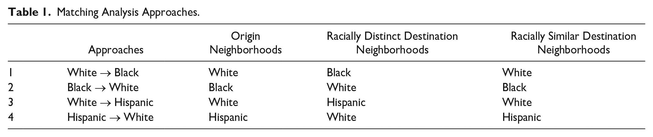
The choice to investigate these two types of racial divisions, Black/White and Hispanic/White, follows from a large body of literature on racial segregation in the United States. The residential dissimilarity between these two sets of groups is overwhelmingly the strongest (Reardon et al. 2008). Furthermore, these three racial groups constitute the majority group in nearly all neighborhoods that have majority groups.

Besides matching on origin neighborhood, the main other matched variables applied are intended to measure how quickly one can travel from one neighborhood to the other: driving time, walking time, and public transportation travel time. Given macrosegregation, majority-white neighborhoods are often substantially separated from majority-nonwhite neighborhoods. It is not surprising to expect that homophily in neighborhood patterns exists, as ties are inherently stronger between closer neighborhoods. By matching dyads into exact bins at the intersection of origin neighborhood, driving, walking, and public transportation travel time, I can approximately compare equally accessible neighborhoods of different racial categorizations, thus providing a refined estimate of the marginal effect of racial composition on the number of visits a neighborhood receives.

The specific matched-pairs design approach used is CEM, a quasi-experimental matched-pairs design that estimates the marginal effect of a particular variable, net of a set of coarsened covariates (Iacus, King, and Porro 2012). CEM works by binning observations in strata that reflect exact combinations of coarsened confounding variables. In this way, matched observations are exact matches across all stratum variables. Unmatched observations are dropped from the analysis. In this case, matched observations are reweighted to reflect how over- or underrepresented racially similar or racially distinct neighborhoods are within their stratum.

I choose to apply CEM in this analysis because it effectively reduces the imbalance in covariates between racially similar and racially distinct neighborhood dyads. In particular, the main otherwise imbalanced covariates of interest here are driving, walking, and public transportation travel time. When comparing how individuals make visits to neighborhoods of different racial compositions, substantial imbalances in travel times between neighborhood groups tend to exist. By taking directed neighborhood dyads and matching exactly on origin neighborhood and coarsened travel times to destination neighborhoods, I seek to balance out travel times between different types of neighborhoods, thus producing estimates of the marginal effect of neighborhood racial composition on visit patterns, net of travel time. Although an alternative approach might be to use traditional regression approaches to control away the effect of travel time, I choose a matching approach here instead, as the assumptions surrounding the relationship between the covariates and the outcome of interest tend to be more flexible (Iacus et al. 2012).

Figures 1 and 2 illustrate the application of the matched-pairs design here visually. For this specific White neighborhood in Baton Rouge, Louisiana, Figure 1 shows the White and Black neighborhoods that can be reached in less than 10 minutes of driving from the referenced origin neighborhood. If I were to match just on origin neighborhood and driving time, the identified neighborhoods would all be considered exact matches of one another. Figure 2 illustrates what some matches might look like if I were to coarsen on the basis of origin neighborhood, driving, walking, and public transportation travel time. The neighborhoods identified there can all be accessed from the origin neighborhood in less than 10 minutes of driving, less than 20 minutes of walking, and between 10 and 20 minutes using public transportation.

Figure 1.

Example of matching on driving time (Tennekes 2018).

Figure 2.

Example of matching on driving, walking, and public transportation time (Tennekes 2018).

I specifically estimate an AME⁴ of neighborhood racial composition on logged visit patterns (Iacus et al. 2012). Exponentiated, this AME can be interpreted as a ratio of visits received between the racially distinct neighborhood category and the racially similar neighborhood category. A ratio less than 1 indicates that after adjusting for the coarsened covariates, racially distinct neighborhoods receive fewer visits than racially similar neighborhoods, whereas a value greater than 1 indicates the inverse. I would reiterate that although CEM constitutes a quasi-experimental method often used to make causal claims, I am not seeking to make causal claims in these analyses. Instead, I am taking advantage of this method to produce a balance in travel time (and other coarsened covariates) between different categories of neighborhoods, thus isolating a more insightful estimate of the marginal effect of racial composition. More details on the application of CEM can be found in the Online Appendix.

Robustness to Additional Controls

In other approaches, I also consider additional confounding variables in creating strata. Specifically, I look at neighborhood residential population, the number of points of interest (POIs) located in the neighborhood, the socioeconomic status of a neighborhood’s residents, and the level of crime in a neighborhood. As an unadjusted reference, I also produce estimates on the basis of strata constructed only on the origin neighborhood (not including driving or any other variables). Table 2 shows the various matched variables I use in this analysis.

Table 2.

Coarsened Matching Variables.

Origin	Dyad Characteristics			Destination Characteristics
Origin Neighborhood	Driving Time	Walking Time	Public Transportation Time	Population	Number of POIs	Poverty Rate	Gun Violence (2017–2019)
	0–10 minutes	0–20 minutes	0–10 minutes	<1,000	<5	>5%	0 incidents
	10–20 minutes	20–40 minutes	10–20 minutes	1,000–2,000	5–20	5%–20%	1 incident
	20–30 minutes	40–60 minutes	20–30 minutes	>2,000	>20	>20%	≥2 incidents
	30–40 minutes	60–80 minutes	30–40 minutes
	40–50 minutes	80–100 minutes	40–50 minutes
	50–60 minutes	100–120 minutes	50–60 minutes
		>120 minutes	>60 minutes/inaccessible

Note: POI = point of interest.

Neighborhoods are grouped into small, medium, and high population groups on the basis of cutoffs of 1,000 and 2,000 residents. Similarly, neighborhoods are grouped into small, medium, and high POI groups on the basis of cutoffs of 5 and 20 total POIs. Additionally, neighborhoods are grouped into small, medium, and high poverty groups on the basis of cutoffs of 5 percent and 20 percent of residents in poverty. Last, neighborhoods are grouped into small, medium, and high crime groups on the basis of cutoffs of one and two gun violence incidents total from 2017 to 2019.

Demographic data for all neighborhoods were obtained from the 2015–2019 five-year American Community Survey estimates. POI data were obtained from SafeGraph’s Point-of-Interest database. Data on gun violence were obtained by geocoding scraped data from the Gun Violence Archive Web site.

Commuting Zone Analysis

I additionally perform two analyses at the commuting zone level. Commuting zones, in many cases, approximate metropolitan statistical areas, which are the focal geographical scale at which racial segregation is analyzed. Racial residential segregation sharply varies among metropolitan areas (Bruch 2014; Reardon et al. 2008), and it has been argued that racial biases and preferences vary between them as well (Clark 2009; Hehman et al. 2019). I use commuting zones here instead of metropolitan areas because commuting zones are the focal geographical unit at which mobility networks are isolated and disconnected from one another (Levy et al. 2020, 2022).

In this set of two analyses, I first investigate how the AME varies between community zones. I use the same approach as described previously, but rather than estimating visit ratios for the pooled set of nationwide observations, I look only at the set of observations for each commuting zone specifically. In producing only one set of these estimates, I only apply one straightforward CEM approach for simplicity: coarsening on the intersection of origin neighborhood and driving time. I refer to the AME estimated for each commuting zone as visit bias.

I additionally use a novel measure, the driving segregation index (DSI), which approximates how easily reachable different types of neighborhoods are within a commuting zone:

D S I_{a b i} = \ln (\frac{p r_{i}}{\sum^{} \frac{p_{j}}{n}})

(2)

where pr_i is the proportion of all neighborhoods in the commuting zone that are group b neighborhoods⁵; p_j is, for a group a neighborhood, the proportion of neighborhoods reachable from neighborhood j in less than 10 minutes of driving; and n is the total number of group a neighborhoods in the commuting zone. This value can essentially be interpreted as how proximal one type of a neighborhood is to another neighborhood, controlling on how common that type of neighborhood is. For example, a high DSI value implies that very few group b neighborhoods are proximal to group a neighborhoods, while a low DSI value implies that many group b neighborhoods are proximal to group a neighborhoods.

DSI is the principal variable used to predict commuting zone–level visit ratios. Other variables also included in the model are anti-Black explicit bias, percentage Black, percentage Hispanic, and between-race inequality. Anti-Black explicit bias is estimated from Project Implicit’s race implicit association test by subtracting how “warmly” non-Hispanic White subjects reported they feel toward Blacks from how warmly they feel toward Whites.⁶ Between-race inequality is estimated as the per capita non-Hispanic White income divided by the per capita non-Hispanic Black (or Hispanic) income.

The following function depicts the mathematical formula for an additional outcome variable, out-group everyday exposure:

E X P_{a b i} = \ln (\sum^{} \frac{v_{j a}}{(v_{j a} + v_{j b}) * n})

(3)

where v_ja is the number of visits from a neighborhood j to group a neighborhoods, v_jb is the number of visits from a neighborhood j to group b neighborhoods, and n is the number of group b neighborhoods in a commuting zone i.

This variable is intended to operationalize realized out-group contact in everyday mobility. Essentially, it approximates the logged percentage of visits made by group b neighborhoods to group a neighborhoods rather than visits to group b neighborhoods. A high exposure implies that group b neighborhoods make more visits to group a neighborhoods than group b neighborhoods, whereas a low exposure implies the opposite.

Results

Primary Analysis

Table 3 presents my main results, where I present exponentiated AMEs. These values can be interpreted as the effect of neighborhood racial categorization on the relative number of visits a neighborhood receives from a given type of origin neighborhood. My unadjusted model examines how residents make visits to other neighborhoods within one-hour driving time and in the same commuting zone, stratifying only on the specific origin neighborhood. Row 1 in Table 3 presents the visit ratios associated with these unadjusted models. As an example of how to interpret these results, the corresponding value for “White → Black,” 0.345, indicates that residents of White neighborhoods visit Black neighborhoods at approximately one third the frequency they visit other White neighborhoods.

Table 3.

Overall Visit Ratios.

	Neighborhood Pairs (Origin → Destination)
Matching approach	W → B	B → W	W → H	H → W
Unadjusted	.345	.201	.451	.227
Driving	.46	.66	.559	.704
Driving + walking + public transit	.493	.82	.585	.873
Driving + points of interest	.575	.517	.574	.69
Driving + population	.516	.598	.582	.739
Driving + poverty	.444	.755	.547	.758
Driving + crime	.375	.895	.508	.804
Number of observations	100,757,750	25,090,350	104,834,129	43,497,118

Note: For the neighborhood pairs, W represents White, B represents Black, and H represents Hispanic neighborhoods. These values can be interpreted as the ratio of visits made to the racially distinct neighborhoods relative to the racially similar neighborhoods. Racially similar neighborhoods always align with the labeled “destination” neighborhood, while racially distinct neighborhoods always align with the labeled “origin” neighborhood. For example, the value for “W → B” refers to the estimated ratio of the number of visits a Black neighborhood receives from a White neighborhood relative to the number of visits received by a matched White neighborhood. The number of observations is effectively lower for some matching approaches because of unmatched observations receiving a weight of zero.

These unadjusted results generally suggest that Black and Hispanic neighborhoods actually have somewhat more homophilous visit tendencies than White neighborhoods. However, it should be noted that Black and Hispanic neighborhoods make up a much smaller proportion of neighborhoods in a commuting zone and tend to be spatially clustered together. White neighborhoods tend to be spread much farther and wider in a commuting zone. Thus, a Black or Hispanic neighborhood may appear to have a much stronger affinity to visiting other Black or Hispanic neighborhoods in the commuting zone simply because it will be much more proximal to them. White neighborhoods may not show such stark patterns because another randomly chosen White neighborhood simply may not be as close.

Net of travel times and general attractiveness, I still see strong homophily between neighborhood types. White neighborhoods especially are more biased toward Black and Hispanic neighborhoods than vice versa. As row 2 in Table 3 shows, matching on driving time only slightly attenuates the ratio of visits to Black and Hispanic neighborhoods that residents of White neighborhoods make relative to other White neighborhoods (0.460 vs. 0.345 and 0.559 vs. 0.451). Distinctly, matching on driving time has a substantial impact on the likelihood of residents of Black and Hispanic neighborhoods to make visits to White neighborhoods. Although residents of Black neighborhoods make only about one fifth (0.201) as many visits to White neighborhoods as they do to other Black neighborhoods, matching on driving time reduces this difference to two thirds (0.660). A similar effect is observed for Hispanic neighborhoods, for which matching on driving time reduces the visit ratio between Hispanic and White neighborhoods from 0.227 to 0.704.

Notably, matching on accessibility by walking and public transportation further attenuates homophily for all groups, but especially for Black and Hispanic neighborhoods. These findings highlight how walking and public transportation accessibility serve to structurally segregate racial groups, even net of driving-based accessibility. Although my unadjusted AMEs suggest that Black and Hispanic neighborhood residents are especially averse to visiting White neighborhoods, I find that net of travel time, these residents are only 18 percent (0.820) and 13 percent (0.873) less likely to visit an equally accessible White neighborhood. Distinctly, Whites are more than twice as likely to visit an equally accessible White neighborhood compared with a Black one and almost twice as likely to visit a White one compared with a Hispanic one.

Neighborhood amenities, in the form of the number of POIs, explain some of White neighborhoods’ homophily. Distinctly, though, I do find that stratifying on POIs, substantially increase Black neighborhoods’ homophilous visit tendencies. Stratifying on population similarly explains some of White neighborhoods’ homophily but strengthens homophily among Black neighborhoods.

Stratifying on poverty only slightly shifts Whites’ tendency to visit Black and Hispanic neighborhoods. Given that Black and Hispanic neighborhoods are generally much poorer than White neighborhoods, this finding suggests that socioeconomic status is not explaining White neighborhoods’ strong homophily. Stratifying on poverty does substantially reduce Black neighborhoods’, and to a smaller extent Hispanic neighborhoods’, homophily. This would imply that Black and Hispanic neighborhoods tend to visit poorer neighborhoods.

Stratifying on crime has a similar effect. Homophily among White neighborhoods is actually slightly stronger once one stratifies on crime. Given that White neighborhoods generally have lower levels of crime compared with Black and Hispanic neighborhoods, this implies that residents of White neighborhoods are more likely to have even more racially homophilous patterns in safe neighborhoods. Distinctly, I find that Black neighborhoods have less racially homophilous visit tendencies stratifying on crime. This implies that Black neighborhoods’ propensity to visit more dangerous neighborhoods explains a sizable share of their racialized visit patterns. It should be noted, however, that the level of crime in a neighborhood may likely be a consequence of who visits the neighborhood rather than a cause (Levy et al. 2020).

Ultimately, several results here are rather striking. Although only 22.6 percent and 24.4 percent of White neighborhoods’ visit tendencies toward Black and Hispanic neighborhoods are attenuated by stratifying on driving, walking, and public transportation travel time, 77.5 percent and 83.6 percent of Black and Hispanic neighborhoods’ visit tendencies are. In simpler terms, the proclivity of White neighborhood residents to not visit Black and Hispanic neighborhoods has very little to do with accessibility. For residents of Black and Hispanic neighborhoods, however, accessibility drives almost the entire gap.

Neighborhoods with High Public Transportation Use

Additionally, I specifically examine public transportation–accessible neighborhoods. These neighborhoods are defined as those where more than 5 percent of the population uses public transportation to get to work.⁷ Table 4 displays these findings. The results for White origin neighborhoods here are quite striking. Residents of these White neighborhoods demonstrably go out of their way to avoid Black and Hispanic neighborhoods. The fact that stratifying on accessibility increases homophily indicates that bias on the part of White neighborhoods is actually a vastly larger factor than accessibility.

Table 4.

Visit Ratios among Neighborhoods with High Public Transportation Use.

	Neighborhood Pairs (Origin → Destination)
Matching approach	W → B	B → W	W → H	H → W
Unadjusted	.562	.197	.72	.257
Driving	.481	.655	.613	.674
Driving + walking	.521	.82	.669	.886
Driving + public transit	.501	.798	.614	.844
Driving + walking + public transit	.535	.873	.667	.906
Number of observations	5,050,971	984,192	5,743,774	1,778,338

Distinctly, accessibility is clearly the dominant factor that separates Black and Hispanic neighborhoods from visiting White neighborhoods. Furthermore, driving, walking, and public transportation inaccessibility all independently contribute to these disparities.

Robustness Analysis

The preceding analyses were also done with a stricter neighborhood operationalization. The stricter operationalization involved requiring a neighborhood to be more than three quarters White, Black, or Hispanic to be classified as such. These results essentially follow the prior results, with homophilic patterns being starker across the board. Tables S1 and S2 in the Online Appendix present these visit ratios.

Commuting Zone Analysis

Table 5 presents the results of the first commuting zone analysis. Models 1 and 2 estimate how much residents of White neighborhoods tend to visit Black neighborhoods relative to equally driving accessible White neighborhoods. The central variable of interest here is the commuting zones’ DSIs (abbreviated WB-DSI and WH-DSI in the table). Model 1 indicates that DSI is positively correlated (significant at p < .01) with the ratio of visits made to Black versus White neighborhoods by residents of White neighborhoods. This indicates that the Black-White DSI predicts less bias in visits. In other words, in commuting zones where Black neighborhoods are less accessible from White neighborhoods, residents of White neighborhoods practice less racial discrimination in their visits. Controlling on percentage Black in model 2 attenuates this finding to marginal significance, though it should be noted that percentage Black and WB-DSI are fairly collinear. I additionally find that between-race inequality (abbreviated WB-BRI in the table) reduces equitability in visits.

Table 5.

Ordinary Least Squares Models Predicting Commuting Zone Visit Ratios.

	Majority Black		Majority Hispanic
	Model 1	Model 2	Model 3	Model 4
Intercept	.428	.203	−.660***	−.750***
Intercept	(.504)	(.515)	(.116)	(.172)
Explicit bias	.090	.079	.238	.252
Explicit bias	(.218)	(.216)	(.232)	(.234)
WB-DSI	.297**	.202⁺
WB-DSI	(.109)	(.121)
% Hispanic	−1.701*	−1.170		.470
% Hispanic	(.675)	(.736)		(.656)
WB-BRI	−.646*	−.650*
WB-BRI	(.253)	(.250)
% Black		1.180⁺	−1.476*	−1.280
% Black		(.689)	(.704)	(.757)
WH-DSI			.390***	.356***
WH-DSI			(.090)	(.102)
WH-BRI			.020	−.001
WH-BRI			(.025)	(.038)
n	84	84	91	91
R ²	.153	.184	.229	.234
Adjusted R²	.110	.131	.193	.189

Note: Values in parentheses are standard errors. WB-BRI = White-Black between-race inequality; WB-DSI = White-Black driving segregation index; WH-BRI = White-Hispanic between-race inequality; WH-DSI = White-Hispanic driving segregation index.

p < .10. *p < .05. **p < .01. ***p < .001.

Models 3 and 4 estimate how often residents of White neighborhoods visit other Hispanic neighborhoods relative to equally driving accessible White neighborhoods. These results show an even more substantial effect of DSI. Of importance here, DSI is the only significant coefficient in either model, thus demonstrating its value as a predictor.

Table 6 presents models estimating how often residents of White neighborhoods visit majority-Black and majority-Hispanic neighborhoods. All variables here are logged, and independent variables are scaled for ease of interpretation. As one would expect, the proportion of neighborhoods that are majority-Black or majority-Hispanic in a neighborhood explains most of the variation in how often residents of White neighborhoods visit majority-Black or majority-Hispanic neighborhoods. This is indicated both by the significant coefficients (p < .001) and high adjusted R² values (.860 and .878) in models 1 and 3, in which it serves as the sole predictor. I also find DSI and visit bias to be highly significant predictors, as indicated by models 2 and 4. In both cases, these three variables are able to explain more than 95 percent of the variation. Although the sizes of the coefficients indicate that DSI and visit bias contribute about equally to explaining Whites’ exposure to Black neighborhoods, visit bias is roughly three times as important as DSI in explaining Whites’ exposure to Hispanic neighborhoods. These results highlight the importance of everyday mobility patterns in contributing to experienced segregation. The racially unequal mobility behavior Whites practice each day plays at least as large of a role, if not larger, as that of spatial macrosegregation.

Table 6.

Ordinary Least Squares Models Predicting Commuting Zone Visits to Majority-Black and Majority-Hispanic Neighborhoods.

	Majority Black		Majority Hispanic
	Model 1	Model 2	Model 3	Model 4
Intercept	−4.134***	−4.134***	−4.224***	−4.224***
Intercept	(.070)	(.037)	(.071)	(.035)
% Black NH	1.77 ***	1.540***
% Black NH	(.070)	(.039)
WB-DSI		−.383***
WB-DSI		(.039)
WB visit bias		.454***
WB visit bias		(.039)
% Hispanic NH			1.819***	1.713***
% Hispanic NH			(.072)	(.039)
WH-DSI				−.192***
WH-DSI				(.041)
WH visit bias				.653***
WH visit bias				(.039)
n	84	84	91	91
R ²	.860	.961	.878	.971
Adjusted R²	.858	.959	.877	.970

Note: Values in parentheses are standard errors. % Black NH = percentage of neighborhoods that are majority Black; % Hispanic NH = percentage of neighborhoods that are majority Hispanic; WB-DSI = White-Black driving segregation index; WB visit bias = White-Black visit bias; WH-DSI = White-Hispanic driving segregation index; WH visit bias = White-Hispanic visit bias.

***

p < 0.001.

Discussion

In this work, I have applied CEM to estimate the marginal effect of racial composition on the number of visits a neighborhood receives from other types of neighborhoods. Three key findings stand out. First, residents of White neighborhoods disproportionality visit other White neighborhoods, and this tendency persists net of accessibility, suggesting that Whites practice strongly racialized proclivities in their everyday mobility patterns. Second, although Black and Hispanic neighborhoods demonstrate stronger homophily in their visit patterns than White neighborhoods in unadjusted terms, these patterns can be explained almost entirely by driving, walking, and public transportation accessibility. Third, bias in visit patterns varies between commuting zones, and Whites appear to “make up” for a lack of racial macrosegregation by practicing greater racialized discretion in visit patterns.

A large body of literature has documented Whites’ discomfort in Black and Hispanic neighborhoods; research has shown that Whites have extremely low residential preferences for Black and Hispanic neighborhoods, which are not entirely mirrored in the opposite direction. This work contributes to that literature by demonstrating that residents of White neighborhoods will visit an equally accessible White neighborhood about twice as often as they will visit an equally accessible Black or Hispanic neighborhood. Moreover, this effect appears to be highly robust to other control characteristics of the destination neighborhood, including residential population, neighborhood attractions, poverty, and crime.

These analyses additionally reveal that Black and Hispanic neighborhoods are hugely segregated from White neighborhoods via lack of driving, walking, and public transportation accessibility. Although the average Black or Hispanic neighborhood visits White neighborhoods only about one fifth as often as they visit other Black or Hispanic neighborhoods, a Black or Hispanic neighborhood is only 18 percent and 13 percent less likely to visit a White neighborhood net of driving, walking, and public transportation travel time. Importantly, walking and public transportation accessibility appear to each contribute to this structural inequality, net of driving accessibility, which is the more evident force for White neighborhoods.

The commuting zone analysis reveals a key finding in the relationship between macrosegregation and visit disparities. For Whites, racially discriminatory visit patterns are a practice that supplements macrosegregation. In commuting zones where Black and Hispanic neighborhoods are already very separate, Whites practice less discretion in their visits. Inversely, more everyday visit discrimination appears to occur in commuting zones where Black and Hispanic neighborhoods can be reached quickly from White neighborhoods. This finding contributes to a broader literature on how segregation is maintained. Substantial research documents Whites’ aversion to Blacks and Hispanics, with Whites strongly preferring to reside in all-White neighborhoods and quickly moving out of a neighborhood when the minority population increases (Farley et al. 1997; Krysan et al. 2009; Krysan and Farley 2002; Sampson and Sharkey 2008). When it comes to everyday mobility, assuming that Whites are similarly averse to visiting as they are to residing in non-White neighborhoods, my results suggest that Whites adopt racially biased visit patterns as a secondary strategy in addition to residential macrosegregation. The systematic effect of these two practices is that Whites have low levels of contact with majority-Black and majority-Hispanic neighborhoods anywhere across the United States.

Last, this work further substantiates the importance of mobility patterns in urban sociological research. Although an enormous body of research bases racial segregation measures on residential racial segregation, this article shows that in terms of everyday contact, unequal visit patterns can dominate and mitigate residential racial segregation in producing the consequential racial segregation found in everyday contexts. Subsequently, research focusing on strictly residential behaviors may considerably misestimate realized everyday segregation and may misjudge its variation between metropolitan areas.

Supplemental Material

sj-docx-1-srd-10.1177_23780231231169261 – Supplemental material for Racial Segregation in Everyday Mobility Patterns: Disentangling the Effect of Travel Time

Supplemental material, sj-docx-1-srd-10.1177_23780231231169261 for Racial Segregation in Everyday Mobility Patterns: Disentangling the Effect of Travel Time by Karl Vachuska in Socius

Footnotes

Acknowledgements

I would like to gratefully acknowledge and thank Brian Levy for reviewing earlier drafts of this article. I would also like to thank Max Besbris for productive discussions and helpful comments on this project.

ORCID iD

Karl Vachuska

Supplemental Material

Supplemental material for this article is available online.

1

Commuting zone size here is operationalized as the number of unique census block groups in the commuting zone.

2

Location data analysis was provided by TravelTime ().

3

The data source for this estimate is the 2015–2019 American Community Survey five-year estimates.

4

Otherwise known as an “average treatment effect.” I use the term average marginal effect” here because I am not making causal claims, as well as because it is problematic to have neighborhood racial composition play the role of a “treatment” variable, as race is nonmanipulable ().

5

Per the original earlier operationalization, group a or group b neighborhoods are either majority-White, majority-Black, or majority-Hispanic neighborhoods.

6

This follows identically from the approach used in several other publications, including Hehman, Flake, and Calanchini (2018) and

7

And those for which the API returned public transportation data.

Author Biography

Karl Vachuska is a graduate student in the Department of Sociology at the University of Wisconsin–Madison. He is interested in neighborhoods, social stratification, and demography.

References

Bastomski

Sara

Brazil

Noli

Papachristos

Andrew V.

2017. “Neighborhood Co-offending Networks, Structural Embeddedness, and Violent Crime in Chicago.” Social Networks 51:23–39.

Besbris

Max

Faber

Jacob William

Rich

Peter

Sharkey

Patrick

. 2015. “Effect of Neighborhood Stigma on Economic Transactions.” Proceedings of the National Academy of Sciences 112(16):4994–98.

Billingham

Chase M.

Hunt

Matthew O.

2016. “School Racial Composition and Parental Choice: New Evidence on the Preferences of White Parents in the United States.” Sociology of Education 89(2):99–117.

Bruch

Elizabeth E.

2014. “How Population Structure Shapes Neighborhood Segregation.” American Journal of Sociology 119(5):1221–78.

Bursell

Moa

Jansson

Fredrik

. 2018. “Diversity Preferences among Employees and Ethnoracial Workplace Segregation.” Social Science Research 74:62–76.

Candipan

Jennifer

Phillips

Nolan Edward

Sampson

Robert J.

Small

Mario

. 2021. “From Residence to Movement: The Nature of Racial Segregation in Everyday Urban Mobility.” Urban Studies 58(15):3095–3117.

Chetty

Raj

Hendren

Nathaniel

Jones

Maggie R.

Porter

Sonya R.

2020. “Race and Economic Opportunity in the United States: An Intergenerational Perspective.” Quarterly Journal of Economics 135(2):711–83.

Clark

William A. V.

2009. “Changing Residential Preferences across Income, Education, and Age: Findings from the Multi-city Study of Urban Inequality.” Urban Affairs Review 44(3):334–55.

Farley

Reynolds

Fielding

Elaine L.

Krysan

Maria

. 1997. “The Residential Preferences of Blacks and Whites: A Four-Metropolis Analysis.” Housing Policy Debate 8(4):763–800.

10.

Giraud

2019. “osrm: Interface between R and the Open Street Map-Based Routing Service.” Retrieved from https://github.com/rCarto/osrm.

11.

Goldsmith

Pat Rubio

. 2016. “Perpetuation Theory and the Racial Segregation of Young Adults.” Social Science Research 56:1–15.

12.

Graif

Corina

Lungeanu

Alina

Yetter

Alyssa M.

2017. “Neighborhood Isolation in Chicago: Violent Crime Effects on Structural Isolation and Homophily in Inter-neighborhood Commuting Networks.” Social Networks 51:40–59.

13.

Hailey

Chantal A.

2022. “Racial Preferences for Schools: Evidence from an Experiment with White, Black, Latinx, and Asian Parents and Students.” Sociology of Education 95(2):110–32.

14.

Hehman

Eric

Calanchini

Jimmy

Flake

Jessica K.

Leitner

Jordan B.

2019. “Establishing Construct Validity Evidence for Regional Measures of Explicit and Implicit Racial Bias.” Journal of Experimental Psychology: General 148(6):1022.

15.

Hehman

Eric

Flake

Jessica K.

Calanchini

Jimmy

. 2018. “Disproportionate Use of Lethal Force in Policing Is Associated with Regional Racial Biases of Residents.” Social Psychological and Personality Science 9(4):393–401.

16.

Hipp

John R.

Perrin

Andrew J.

2009. “The Simultaneous Effect of Social Distance and Physical Distance on the Formation of Neighborhood Ties.” City & Community 8(1):5–25.

17.

Iacus

Stefano M.

King

Gary

Porro

Giuseppe

. 2012. “Causal Inference without Balance Checking: Coarsened Exact Matching.” Political Analysis 20(1):1–24.

18.

Joyner

Kara

Kao

Grace

. 2000. “School Racial Composition and Adolescent Racial Homophily.” Social Science Quarterly 81(3):810–25.

19.

Krysan

Maria

Bader

Michael D. M.

2009. “Racial Blind Spots: Black-White-Latino Differences in Community Knowledge.” Social Problems 56(4):677–701.

20.

Krysan

Maria

Couper

Mick P.

Farley

Reynolds

Forman

Tyrone A.

2009. “Does Race Matter in Neighborhood Preferences? Results from a Video Experiment.” American Journal of Sociology 115(2):527–59.

21.

Krysan

Maria

Farley

Reynolds

. 2002. “The Residential Preferences of Blacks: Do They Explain Persistent Segregation?” Social Forces 80(3):937–80.

22.

Levy

Brian L.

Phillips

Nolan E.

Sampson

Robert J.

2020. “Triple Disadvantage: Neighborhood Networks of Everyday Urban Mobility and Violence in US Cities.” American Sociological Review 85(6):925–56.

23.

Levy

Brian L.

Vachuska

Karl

Subramanian

S. V.

Sampson

Robert J.

2022. “Neighborhood Socioeconomic Inequality Based on Everyday Mobility Predicts COVID-19 Infection in San Francisco, Seattle, and Wisconsin.” Science Advances 8(7):eabl3825.

24.

Lundberg

Ian

. 2022. “The Gap-Closing Estimand: A Causal Approach to Study Interventions that Close Disparities across Social Categories.” Sociological Methods & Research. doi:10.1177/00491241211055769.

25.

Massey

Douglas S.

Denton

Nancy A.

1993. “American Apartheid: Segregation and the Making of the Underclass.” Pp. 660–70 in Social Stratification, Class, Race, and Gender in Sociological Perspective, edited by Grusky

New York: Routledge.

26.

OpenStreetMap. OSM History Dump © OpenStreetMap Contributors. Retrieved July 15, 2022. https://planet.openstreetmap.org/planet/full-history/.

27.

Rader

Nicole E.

May

David C.

Goodrum

Sarah

. 2007. “An Empirical Assessment of the “Threat of Victimization:” Considering Fear of Crime, Perceived Risk, Avoidance, and Defensive Behaviors.” Sociological Spectrum 27(5):475–505.

28.

Reardon

Sean F.

Matthews

Stephen A.

O’Sullivan

David

Lee

Barrett A.

Firebaugh

Glenn

Farrell

Chad R.

Bischoff

Kendra

. 2008. “The Geographic Scale of Metropolitan Racial Segregation.” Demography 45(3):489–514.

29.

Sampson

Robert J.

Sharkey

Patrick

. 2008. “Neighborhood Selection and the Social Reproduction of Concentrated Racial Inequality.” Demography 45(1):1–29.

30.

Schaefer

David R.

2012. “Youth Co-offending Networks: An Investigation of Social and Spatial Effects.” Social Networks 34(1):141–49.

31.

Small

Mario L.

Akhavan

Armin

Torres

Wang

. 2021. “Banks, Alternative Institutions and the Spatial–Temporal Ecology of Racial Inequality in US Cities.” Nature Human Behaviour 5(12):1622–28.

32.

Stearns

Elizabeth

. 2010. “Long-Term Correlates of High School Racial Composition: Perpetuation Theory Reexamined.” Teachers College Record 112(6):1654–78.

33.

Tennekes

Martijin

. 2018. “tmap: Thematic Maps in R.” Journal of Statistical Software 84(6):1–39. doi:10.18637/jss.v084.i06

34.

Thibodeaux

Jarrett

. 2016. “City Racial Composition as a Predictor of African American Food Deserts.” Urban Studies 53(11):2238–52.

35.

Vachuska

Karl

. 2023. “Neighborhood Racial and Economic Composition Predicts Incidence of Various Emergency Service Responses.” Socius 9: 23780231231157679.

36.

Vachuska

Karl

Levy

Brian

. 2022a. “Neighborhood Disadvantage Based on Everyday Mobility Predicts Intrauterine Growth Restriction for Black and Hispanic Births in California.” Presented at the PAA 2022 Annual Meeting; April 6–9; Atlanta, Georgia.

37.

Vachuska

Karl

Levy

Brian

. 2022b. “Neighborhood Racial and Economic Composition Predicts Risk of Police Killing.” Presented at the PAA 2022 Annual Meeting; April 6–9; Atlanta, Georgia.

38.

Vachuska

Karl

Movahed

Masoud

. 2022. “Estimating the Causal Effect of Gun Violence on Neighborhood Popularity.” Working Paper. Madison: University of Wisconsin–Madison.

39.

Wang

Phillips

Nolan Edward

Small

Mario L.

Sampson

Robert J.

2018. “Urban Mobility and Neighborhood Isolation in America’s 50 Largest Cities.” Proceedings of the National Academy of Sciences 115(30):7735–40.

40.

Wells

Amy Stuart

Crain

Robert L.

1994. “Perpetuation Theory and the Long-Term Effects of School Desegregation.” Review of Educational Research 64(4):531–55.

41.

Wilson

William Julius

. 1987. The Truly Disadvantaged: The Inner City, the Underclass, and Public Policy. Chicago: University of Chicago Press.

42.

Wimmer

Andreas

Lewis

Kevin

. 2010. “Beyond and below Racial Homophily: ERG Models of a Friendship Network Documented on Facebook.” American Journal of Sociology 116(2):583–642.

43.

Zenk

Shannon N.

Schulz

Amy J.

Israel

Barbara A.

James

Sherman A.

Bao

Shuming

Wilson

Mark L.

2005. “Neighborhood Racial Composition, Neighborhood Poverty, and the Spatial Accessibility of Supermarkets in Metropolitan Detroit.” American Journal of Public Health 95(4):660–67.

Supplementary Material

Please find the following supplemental material available below.

For Open Access articles published under a Creative Commons License, all supplemental material carries the same license as the article it is associated with.

For non-Open Access articles published, all supplemental material carries a non-exclusive license, and permission requests for re-use of supplemental material or any part of supplemental material shall be sent directly to the copyright owner as specified in the copyright notice associated with the article.

0.00 MB

0.02 MB