Sage Journals: Discover world-class research

Abstract

Prediction is an underused tool in the social sciences, often for the wrong reasons. Many social scientists confuse prediction with unnecessarily complicated methods or with narrowly predicting the future. This is unfortunate. When we view prediction as the simple process of evaluating a model’s ability to approximate an outcome of interest, it becomes a more generally applicable and disarmingly simple technique. For all its simplicity, the value of prediction should not be underestimated. Prediction can address enduring sources of criticism plaguing the social sciences, like a lack of assessing a model’s ability to reflect the real world, or the use of overly simplistic models to capture social life. The author illustrates these benefits with empirical examples that merely skim the surface of the many and varied ways in which prediction can be applied, staking the claim that prediction is a truly illustrious “free lunch” that can greatly benefit social scientists in their empirical work.

Keywords

prediction computational social sciences explanation

Social scientists should start using prediction more often. Prediction is the process of generating predicted values of a dependent variable by applying an estimated model to a set of explanatory variables, bringing a unique analytical perspective to empirical work. Prediction can also help address enduring sources of criticism facing the social sciences. Examples are a general lack of assessing research findings in terms of their real-world relevance, and the use of overly simplistic models to study the complexities of social life. In this article, I address common misconceptions about prediction and provide a simple definition that addresses existing barriers to adoption. I then discuss and illustrate some of the many benefits that prediction can bring when used as a complement to traditional empirical methods. I argue that prediction can and should become a fundamental part of the social scientist’s empirical toolkit but that this first requires us to look beyond the current dichotomy between prediction and explanation and instead view the two as complementary to each other.

The current lack of prediction in the social sciences stems from a seeming incompatibility between wanting to explain and wanting to predict, effectively forcing researchers to choose between the two approaches. A case in point is the much-cited article by Galit Shmueli (2010), aptly titled “To Predict or to Explain,” which outlines how a social scientist’s empirical work flow differs in terms of data processing, modeling, and postestimation diagnostics when choosing to either predict or explain. Naturally, Shmueli assumes that a researcher would not normally attempt to do both. This is an accurate reflection of social science research. The apparent need to dogmatically choose between either approach means that, in practice, social scientists tend to stick to explanation almost exclusively. Illustratively, the terms predict and prediction are mentioned in fewer than 5 percent of abstracts over the past 10 years in various flagship journals in economics, political science, and sociology, and of the articles mentioning either term, only 13 percent proceed to generate actual predictions of the outcome variable (Table 1).^1,2

Table 1.

Numbers of Articles Using the Term Predict or Prediction in the Abstract and Actual Use of Prediction in Six Flagship Journals in Economics, Political Science, and Sociology, 2010 to 2021.

Journal	Total Articles^a	Mentions Prediction	Actually Makes Predictions^b
American Economic Review	2414	85	12
Quarterly Journal of Economics	458	47	3
American Journal of Political Science	800	61	14
American Political Science Review	743	33	4
American Journal of Sociology	394	8	0
American Sociological Review	523	24	1

Data were collected using the Scopus API.

Understood as generating predictions of the outcome variable (including forecasting). Articles generating predicted probabilities by setting explanatory variables to their means or medians were excluded because such predictions do not reflect actual observations in the data.

So why does this dichotomy exist? In many cases, an unnecessarily narrow interpretation of prediction is to blame. For example, the type of prediction discussed by Shmueli (2010) refers to the practice of maximizing predictive power, which is a subset of the more general practice of making predictions. As a result, prediction is often conflated with the use of complex nonlinear models such as those from the domain of machine learning, which have their own unique set of challenges (Athey and Imbens 2019). There is no reason to transfer these challenges to the general process of making predictions, which can be done with any type of model. Prediction also tends to be narrowly understood as forecasting, which is but one of numerous examples of making predictions (Watts 2014).³ The biggest culprit, however, is the enduring discussion whether prediction and explanation are conceptually the same, and whether the latter should imply the former. This philosophical debate, although interesting, is ultimately irrelevant to applying prediction in explanatory research. When viewing prediction as a simple tool to evaluate a model’s ability to approximate the outcome of interest, it can be applied without exception to most social science questions, rendering a dogmatic choice between prediction or explanation unnecessary.

The more relevant question is what prediction might bring to the table. To illustrate just one dimension, take the Fragile Families Challenge (FFC), a case to which I will return throughout this article (Salganik et al. 2019). During the FFC, 160 research teams around the globe were asked to predict a number of important early-stage life outcomes of general interest to social scientists (e.g., eviction and material hardship). The idea was to evaluate the general predictability of these outcomes through a common task setup (Donoho 2017). This setup mirrored the popular competition Web site Kaggle, where data sets with some outcome of interest and a number of possible explanatory variables are published online. Participants are challenged to estimate models that can accurately predict the outcome. These models are then tested on a partition of the data, which is kept secret. Similar to Kaggle, the FFC made available a rich data set to generate predictive models, while storing an evaluation set against which each team’s predictive model was scored. The organizers encouraged the use of prediction-focused algorithms, rather than the explanatory methods already applied in hundreds of peer-reviewed articles using the same data.

The conclusions were telling for a number of reasons. First, many teams applied methods using flexible functional forms and variable selection techniques not often seen in the social sciences. Second, most models were nonetheless poorly able to predict life outcomes, although some did improve on benchmark models including a curated number of explanatory variables in a standard linear model. Poor overall predictability was thus a feature of both predictive and explanatory techniques. Third, and most important, the FFC was a rare occasion in which the onus was truly on prediction rather than explanation. As a consequence, it put into sharp focus the fact that decades of explanatory research into the outcomes of interest had not led to much predictive ability. This somewhat awkward finding led the organizers to conclude that researchers had to “find a way to reconcile a widespread belief that understanding has been generated by these data . . . with the fact that the very same data could not yield accurate predictions of these important outcomes” (Salganik et al. 2020:8402).

If prediction had been a more natural tool for social scientists, the main take-away of the FFC would likely not have taken so long to materialize. An earlier realization of the predictive limits of our knowledge might have stimulated a rigorous evaluation of the mechanisms hypothesized, the methods used, and/or data collected at an earlier stage in the data set’s rich academic career and throughout life course research more generally. Importantly, it is unlikely that poor predictability is only a feature of life course research. Assessing the ability of our research findings to meaningfully predict outcomes we are interested in will most likely spur important debate in many other domains as well. The point is that our traditional preference for in-sample diagnostics means that we often do not assess our models ability to approximate the outcomes we care about. Prediction can, among other things, solve this problem.

The FFC is but a single example how prediction can shine a different light on empirical work and represents one of many approaches to making and evaluating predictions. More generally, in this article I argue that prediction can bring the following three key virtues to the table of the social scientist:

Prediction provides improved insight into model fit.

Prediction provides a benchmarking tool across modeling domains.

Prediction can help generate insight into the behavior of complicated models.

These key virtues come in addition to other benefits. Some examples are an improved alignment of research findings and policy (Athey and Imbens 2019), providing a metric to align scientific efforts (Hofman, Sharma, and Watts 2017; Cranmer and Desmarais 2017), and improving transparency and the ability to scrutinize estimated models (Greenhill, Ward, and Sacks 2011). Viewing prediction as a complement to classical methods would also ease the incorporation of prediction-focused methods from machine learning into the social sciences (Rahal, Verhagen, and Kirk 2021).

To summarize, in this article I aim to increase the use of prediction in explanatory research by challenging the unnecessary dichotomy between prediction and explanation, and illustrating the many benefits prediction brings when applied as a complement to explanatory analysis. Hopefully, this article can serve as a pragmatic guide to the varied ways in which prediction can be successfully applied in the social sciences. The remainder of this article is structured as follows. First, I discuss several reasons why prediction is currently being underused and provide a definition of prediction that should address these obstacles to adoption. I then provide a number of ways in which prediction can be operationalized, dependent on the case at hand. To showcase the benefits of prediction, I then present three sets of empirical examples, in line with the three virtues outlined above, to illustrate the application of prediction. I conclude the article with a summary and discussion of the main claims and findings.

A New Perspective on Prediction for the Social Sciences

The social sciences are currently dominated by a focus on explanation. This often boils down to estimating models reflecting some explanatory mechanism and assessing the in-sample coefficient estimates of these models. Prediction—which broadly reflects an interest in how well the models we estimate are able to approximate the dependent variable—plays, at best, an auxiliary role.⁴ In the following discussion, I identify three reasons why a predictive focus in the social sciences is lacking. Then, I provide a simple definition of prediction that should not suffer from such barriers to adoption.

Before doing so, it is appropriate to briefly reflect on the intriguing philosophical debate whether explanation and prediction are conceptually the same. Some authors have forcefully claimed that causal explanation should always have predictive implications (Freedman 1991; Hempel and Oppenheim 1948; Watts 2014), whereas others (equally strongly) qualify this viewpoint (Hedström and Ylikoski 2010). I do not seek to wade into this debate for two reasons: first, because the debate has been documented extensively elsewhere (Breiman 2001; Hofman et al. 2021; Watts 2014), and second, and more important, because the formal (in)equality between prediction and explanation is not strictly required to apply prediction for explanatory purposes. Therefore, I do not aim to support or assume either view going forward and encourage others to take a similarly pragmatic approach when considering to use prediction in their work. In that respect, none of the examples I use in this article requires a strong position on the above.

Prediction Is Often Misperceived as Deterministic Forecasting

Prediction is underused in the social sciences in part because of misperceptions of what prediction actually is. Prediction is often understood to deal with predicting outcomes or events in the future (i.e., outside of the time frame on which we have current data) and to be intrinsically deterministic (i.e., as making statements with certainty). This type of prediction is at best a small subset of the general process of making predictions.⁵

In fact, predictions need not be made on future events, nor must prediction exclusively concern time-varying data. A mechanistic theory describing the effect of some variable X on an outcome y via some model y = f(X) can lead to predictions in future, current, and past cases as long as the data used for prediction are similar to those used in estimating the model. For example, predictions can be made for a small partition of the data set collected to study some mechanism, which is set aside and not used for model estimation but purely for predictive evaluation. This is the typical approach to prediction observed in the field of machine learning (Donoho 2017). Tellingly, most machine learning applications do not concern time-varying events at all (Hastie, Tibshirani, and Friedman 2009). The only thing conceptually required to predict is a set of data similar to that used in estimation.

Accordingly, predictions are made using estimated models and should thus be viewed from a probabilistic perspective, just like classic techniques like (logistic) regression are inherently probabilistic in nature too. What makes prediction different is an explicit focus on the outcome variable. There is no reason to assume determinism any more when making predictions using some model, than determinism is involved when evaluating the estimated coefficients of that very model.

Historical Limitations Limit the Use of Prediction in the Present

Historically, there were considerable limitations on both data and computational resources available to researchers. This still affects the use of prediction in the present. A parallel can be drawn to the enduring imbalance between Bayesian and frequentist approaches to inference in the social sciences. Bayesian statistics require a relative abundance of computational resources, compared with a frequentist approach. This made the use of fairly simplistic linear models—plugged into exponential family probability distributions with computationally convenient properties—the preferred methodological approach for social scientists during the latter half of the twentieth century (Efron and Hastie 2016). This dominance persists up to this very day. Choices that were reasonable and necessary at the time, but which have led to an analytical monoculture today (Hindman 2015).

Making predictions is similarly expensive: in some cases a part of the data set must be put aside for evaluation or models must be estimated many times for robust inferences into the predictive performance of a model. Limits on data and computational resources have thus strengthened a (historical) preference for in-sample inferential methods (Efron and Hastie 2016). In a day and age of ever larger data sets and computational power, these issues are a problem of the past. Just as the increases in both data and computational resources have led to a burgeoning growth of methods using Bayesian approaches, the use of prediction should no longer be held back by practical concerns. Even in small-N settings, techniques are available that still allow prediction to be applied.⁶

Prediction Is Conflated with the Use of Convoluted Models

More recently, prediction is approached with hesitance because of the astronomic rise of techniques from the domain of machine learning that place a strong emphasis on prediction (Hofman et al. 2017; Shmueli 2010). This has led to the risk that the limitations of machine learning methods are blindly transferred to prediction in general. To illustrate, reviews discussing the potential of machine learning for the social sciences have appeared in various important journals (Grimmer, Roberts, and Stewart 2021; Hofman et al. 2017; Molina and Garip 2019; Mullainathan and Spiess 2017). All these reviews discuss the benefits of machine learning (e.g., increased model complexity and the lack of reliance on prespecified functional forms) as well as the key difference: machine learning’s focus on prediction.

Machine learning methods have various limitations and risks associated with them, most notably highly convoluted models with a profound lack of interpretability (Athey 2017).⁷ These risks have little to do with the general process of making predictions. Decoupling prediction from black-box methods is crucial to break the misperception that predictive accuracy is something that is naturally maximized at the cost of interpretability. Predictions can be made as easily using an additive linear model as with the complicated nonlinear algorithms commonly applied in machine learning. That researchers within machine learning almost exclusively predict does not mean that prediction is exclusive to machine learning.

A Simple Definition of Prediction

Prediction understood as the process of evaluating a model in terms of its ability to accurately approximate the outcome should not suffer from the definitional confusion outlined above. Prediction simply calls for a renewed emphasis on our model’s ability to model the dependent variable in our data. On the basis of this definition, making predictions consists of the following simple steps:

Define an estimation set to fit the model and an evaluation set to generate predictions for.

Estimate the model using the estimation set.

Make predictions of the outcome using the model and the data in the evaluation set.

Evaluate the performance of the predictions against the observed outcome.

Clearly, the above subsumes the more narrow definitions of prediction like forecasting, or the use of machine learning, which fall within the confines of this broader definition.

To make the above more concrete, assume we estimate some functional form f_µ(·) in order to find evidence for the association of years of education, A, on wages, y, an example I return to later. We include work experience, B, as a control variable leading to the model y = f_µ(y, A, B). Typically, f_µ(·) is a linear additive model plugged into an exponential family probability distribution with parameter-vector µ, although more complicated algorithms can be applied without loss of generality. Prediction is as simple as estimating ${\hat{f}}_{} (\cdot)$ using information on y^estimation, A^estimation, and B^estimation from some data set D^estimation and generating predictions using information on A^evaluation and B^evaluation from some data set D^evaluation:

{\hat{y}}^{evaluation} = {\hat{f}}_{} (A^{evaluation}, B^{evaluation})

(1)

The predictions ${\hat{y}}^{evaluation}$ can then be evaluated, for example by comparing them against the actually observed y^evaluation. There are many summary metrics of fit available for this purpose (e.g., the root-mean-squared error or F1 score), but one can also compare (sets of) individual predictions against observed outcomes. Of interest is the broad ability of ${\hat{f}}_{} (\cdot)$ to accurately model the outcome.

On the basis of this definition, the only decision a researcher has to make is how to define the set used for estimating the model and how to define the set used to evaluate its predictive performance. I identify three general approaches, which I discuss below.

In-Sample Evaluation

A first option is to simply use the same data used for estimation to make predictions (Figure 1A). This choice would effectively lead to an in-sample assessment of model fit, and the well-known R² is an example of aggregate fit under this choice of evaluation set. A form of in sample prediction is sometimes also applied by researchers interpreting coefficients in nonlinear models where the coefficient estimates lack straightforward interpretation, like categorical outcome models (Breen, Karlson, and Holm 2018; Hanmer and Kalkan 2013).⁸

Figure 1.

Three different strategies to define an estimation set and an evaluation set. The first strategy (A) uses the original data as both the estimation set as well as the evaluation set. The second strategy (B) splits the original data into K splits. Each split is used once as an evaluation set, to evaluate the model estimated to the remaining K – 1 splits. The model is thus estimated K times. This step can be repeated M times, leading to repeated K-fold cross-validation, or Monte Carlo cross-validation in case only a single estimation or evaluation cycle is done per run instead of K (Yousef 2020). The third strategy (C) uses the original data to estimate the model, and uses a different data set to evaluate the model, which can be a holdout set from the same data-generating process (DGP) but partitioned off prior to analysis, or collected separately.

In effect, in-sample evaluation boils down to assessing the fitted values of the model estimated in step 2 given previously. For parametric models with sufficient sample sizes, this is an efficient approach as it uses all the available data for both estimation and evaluation. The downside is the risk that in-sample predictions can be overfit, leading some to argue that predictions should be made exclusively out of sample (Cranmer and Desmarais 2017). Overfitting is the reason why aggregated in-sample fit metrics such as the adjusted R² or information criteria are scaled downward on the basis of the degrees of freedom in a model.⁹ When evaluating predictions at a lower level of aggregation (e.g., for a subset of the data) or when models become more parametrized (e.g., multilevel models or when using regularization techniques) using separate estimation and evaluation sets is strongly advised.

Cross-Validated Evaluation

A second approach is to partition the existing data set into disjunct estimation and evaluation sets. This is the typical approach often observed in machine learning and has the added benefit that any risk for overfitting the data is explicitly addressed. Predictions are only ever made for data that were not used to estimate the model. The most common such approach is K-fold cross-validation, which consists of dividing the data set into K equal-sized “folds”; typically, K is set to 5 or 10. The model is then estimated K times, each time omitting one of the folds from the estimation process and using the omitted fold as the evaluation set (Figure 1B). This ensures that predictions are generated for every observation in the data set, thus maximizing the number of predictions given the available data. It does make the routine computationally more expensive, as the model must be fit K times. K-fold cross-validation also means that estimation is only ever done on n – n_k data points per run, which can lead to a loss in efficiency and precision of the estimates.

There are various alternatives to implementing cross-validation. For example, in low-N situations or when efficiency in estimation is paramount, one could use leave-one-out cross-validation, which is the special case of K-fold cross-validation in which K is set to N (Stone 1974). As the number of folds K approaches N, the loss in efficiency decreases, although the computational cost of performing the cross-validation increases. For relatively straightforward estimation like ordinary least squares, the overall increase in computational time is negligible, but it can become prohibitive if the time required to perform a single estimation of the model is already considerable. Beyond varying the number of folds K, additional robustness to random variation in splitting the data into folds can be incorporated by repeating the entire routine multiple times.¹⁰ Overall, K-fold cross-validation remains the most commonly applied approach.

External Evaluation

A third and final choice for the evaluation set can be a set of data that are completely “unseen” by the researcher (Figure 1C). For example, by immediately partitioning off a part of the data into a holdout set that is kept separate from the entire estimation process or, ideally, never even shared with the researcher(s), which is the typical approach in Kaggle-style competitions. This is called the “holdout” approach and provides the most truthful assessment of a model’s predictive performance. Unfortunately, it is expensive, as a sufficient number of observations are required to make predictions, and these observations cannot be used for estimation, thus leading to both reduced efficiency in estimation and a reduced number of predictions to evaluate.

External validation can also be done by assessing model predictions on a completely new set of collected data. For example, similar data that were collected at a different time (e.g., separate waves of a survey) or place (e.g., regional comparisons). The choice of an external evaluation set speaks directly to calls for increased attention to the external validity of research findings in empirical work (Simonsohn, Simmons, and Nelson 2020; Young 2018) and can be particularly useful to assess the transferability of research findings outside of the sample used for estimation. By choosing an external validation set, prediction provides a simple and direct framework to assess model fit outside of the sample at hand.

In practice, the choice of splitting the data into estimation and evaluation sets will be made on a case-by-case basis. If a parametrized model is estimated with few coefficients and a considerable data size (e.g., N > 500), the risk for overfitting will generally be low, and in-sample prediction could be considered. When the number of parameters in a model increases, it is advisable to use some form of cross-validation, either leave-one-out in case the number of observations is limited or K-fold with K typically about 10 (Kohavi 1995). If N is sufficiently large that setting aside a portion of the data does not meaningfully affect model estimation, the holdout approach can be applied where typically 20 percent to 30 percent of the data are partitioned off as the holdout set.¹¹

When using prediction to improve model understanding, as most of the examples in this article do, leave-one-out cross-validation is generally attractive if computationally feasible. Prediction is out of sample and the maximal number of data points (n – 1) are used to estimate the models used for each prediction. However, when the goal is to select an optimal predictive model to deploy among a set of candidate models, one might be interested in the expected prediction error on a completely new observation and the variability of this prediction error. In this case, K-fold cross-validation is typically a more efficient estimator, although some properties of the estimand are not yet completely understood (Efron and Hastie 2016).¹² The holdout or external validation approach will give the most precise assessment of a model’s ability to accurately predict the outcome of new observations, although it is clearly expensive as one must completely set aside a part of the data for evaluation or collect a new data set. These questions are less relevant when using predictions to improve our understanding of explanatory models, as is the focus in this article.

The Three Virtues of Prediction

As outlined in the introduction, complementing traditional methods with prediction brings three key virtues to the social scientist’s table. In what follows, I illustrate these in kind using examples of prior work and novel reproductions.¹³

Virtue 1: Prediction Provides Improved Insight into Model Fit

In its most simple form, prediction provides a distinct way to assess model fit on the level of the actual outcome variable. Such a perspective provides a renewed focus on what one could call predictive consciousness: an understanding how well our models are actually able to fit the outcome variable of interest. In practice, a model’s fit is often left undiscussed, leading to a broad lack of predictive consciousness in empirical work, for example, whether the models we estimate are able to accurately predict 0.1 percent, 1 percent, or 50 percent of the variation in the outcome. Model fit, if it is discussed at all, is typically assessed at the aggregate level only.¹⁴ We are often left guessing what elements in a model contribute most to its ability to predict well. Nor do we know whether a model is able to predict all of the data equally well or just parts of it. A renewed appreciation for prediction will improve our assessment of model fit, as predictions are made for every single observation in the evaluation set. As a consequence, a (disaggregated) assessment of fit on the scale of the outcome comes naturally.

Predictive performance is also intuitive to understand and will help the implementation of research findings in the real world. Its intuitive nature promotes acceptance and understanding of research findings by both policy makers and the public. Academically, a general sense of predictive accuracy is equally important to further a research agenda: if predictive performance (strongly) underperforms expectations, it prompts reflection of whether we are actually missing important determinants or perhaps our preferred functional form is not able to capture the mechanisms in operation. Finally, making and evaluating predictions beyond the aggregate level can also provide additional transparency into the academic process. By reporting on model fit at lower levels of aggregation, consumers of empirical research become better able to critically assess what a model can and cannot do in terms of fitting the data.

As a first example, consider the FFC, which was introduced earlier (Salganik et al. 2019). The FFC challenged research teams to accurately predict life outcomes at age 15 on the basis of a rich set of data using the holdout approach (i.e., setting aside a partition of the data).¹⁵ As part of the challenge, the organizers calculated a benchmark performance using models constructed by domain experts. As a consequence, the low predictive power of the models typically estimated in this domain already became quite obvious from the outset (Figure 2A). For many of the life outcomes of interest measured at age 15, a model including the handpicked variables and a lagged version of the variable at age 9 did not substantially improve predictive accuracy relative to a null model predicting the overall mean of the outcome. This is a sobering finding putting into perspective the supposedly large amount of understanding that had been generated regarding these outcomes (Salganik et al. 2020).

Figure 2.

(A) Predictive R² of the linear benchmarks chosen by domain experts relative to a null model for the Fragile Families Challenge (FFC). Each model includes four explanatory variables and a lagged version of the outcome (Salganik et al. 2020). (B) Individual predictions of the grade point average (GPA) outcome in the FFC using only the domain expert variables (top) and when including the lagged version of the outcome (bottom). (C) Performance of logistic regression models predicting whether a mortgage application was successful using various sets of explanatory variables. Performance is shown disaggregated for White (green) and non-White (blue) applicants, showing that the performance is considerably lower for the latter. (D) Performance of models predicting students’ track levels using various sets of explanatory variables and different models. Performance of the categorical model is substantially higher than the linear model. The performance of both models strongly increases when including school variation. (E) Performance of various models in explaining hourly wage in the United States. Predictive power is assessed for each year using the same model but reestimated to that year’s data (triangles) or using the model estimated in the year 1973 (stars). Initially, the latter model performs well on the first couple of subsequent waves but deteriorates from 1983 onward. Confidence intervals, where present, reflect 95 percent confidence bounds of the estimated predictive accuracy across the various evaluation folds.

Perhaps the outcomes of interest to the FFC are inherently noisy and difficult to predict, as the organizers also note (Hofman et al. 2017; Salganik et al. 2020). Regardless of the question why predictive ability was low within the FFC, the very insight and subsequent discussion it provoked are essential for the field to develop. The FFC illustrates how predictive consciousness can be crucial to instigate a critical reflection on the state of knowledge in a field and can spur important debate. Accordingly, the key take-away of the FFC is that the type of discussion a predictive focus triggered should not have taken so long to materialize. Likely, a predictive consciousness is equally relevant for many other social science research fields. More consistent reporting of predictive accuracy would guarantee that the type of reflection resulting from the FFC becomes more likely to occur throughout the social sciences.

Predictions can also diagnose model performance at different levels of detail or aggregation. As an example, take the individual predictions rather than the overall predictive accuracy of the benchmark model for the grade point average (GPA) outcome in the FFC. We can visualize the predicted GPA against the observed GPA for each observation in the evaluation set and can do so for different models (Figure 2B). Taking such a disaggregated approach to model fit, we observe that both models struggle to structure the outcome well, but this is especially so for students performing below average. This is a nuance that provides pointers for future avenues of research. In other words, prediction’s ability to interrogate model fit on a disaggregated level provides a different vantage point than summary metrics of model fit.

In addition to individual predictions, they can also be assessed (1) at the group level or (2) using completely different models and/or sets of explanatory variables. As an example, consider a reproduction of the influential 1996 study from the Federal Reserve Bank of Boston regarding discrimination in mortgage lending (Munnell et al. 1996). The authors found, among other things, evidence of discrimination against non-Whites on the basis of a logistic regression including a race dummy and conditioning on various objective characteristics of the application. By complementing their analysis with a predictive perspective, additional nuances emerge (Figure 2C).¹⁶

For example, most individuals are successful in their mortgage applications, and a null model already correctly predicts 88 percent of the data (by predicting successes for everyone). Including variables such as objective score measures and household characteristics further increases the model’s performance. However, aggregate fit is somewhat misleading, as there is a considerable gap in the model’s ability to predict outcomes for non-White applicants compared with White applicants (77 percent vs. 92 percent). The inclusion of a race indicator only marginally improves the gap. In other words, non-Whites are modeled considerably less accurately than Whites. This could imply that additional sources of heterogeneity are present for the former (e.g., if bias is multimodal and depends on other factors, such as the employee reviewing the application) or some other reason is present why non-Whites are modeled considerably less well.

Another illustration in which prediction provides additional understanding of model fit is a recent study assessing teacher bias in educational tracking—the process of assigning students to ability levels—in the Netherlands. In the article, prediction is explicitly applied to understand the relative importance of different sets of explanatory variables as well as modeling assumptions (Verhagen 2021b) (Figure 2D).¹⁷ This predictive perspective led to a number of important nuances to the existing knowledge on teacher bias. First, a predictive approach showed that commonly studied bias factors such as parental education, although statistically significant, mattered little for the model’s fit of the data, improving the predictive R² by a mere 0.1 percent. When allowing for separate intercepts per school, typically perceived as a control variable, the improvement on model fit was considerably greater, increasing the predictive R² by almost 3 percent. Second, using a nonlinear categorical model strongly improved the model’s fit of the data compared with the simpler linear model traditionally estimated in the field.¹⁸

Both nuances have important substantive implications for research on teacher bias, which were not picked up in preexisting work that focused on traditional inference. For example, school effects were typically evaluated through the estimated variance term of the random intercept. They were not typically compared with the other variables in the model with respect to their substantive ability to model the outcomes. As a consequence, a considerable source of variation in tracking had been neglected. Similarly, traditional fit metrics will only indicate an objective preference for the categorical model but do not provide a normative reflection of the extent to which model fit improves. Importantly, changing to the categorical model also considerably affected the size of estimated biases in tracking (Verhagen 2021b).

A final advantage of using prediction as a measure of model fit is that it can be used as an approach to address questions of external validity. A recurring question in the social sciences is the persistence of research findings outside of the particular sample used to estimate a model. Prediction makes such assessments more natural than in-sample methods do. For example, consider the following puzzle in labor economics. A growing literature is studying the reasons underlying an increase in the amount of residual variance over time when explaining logged hourly wages using a similar set of explanatory variables: education, age, and their interactions (Lemieux 2006a). This example lends itself well for an illustration of how the external validity of a model can be assessed from a predictive perspective. By estimating the model on one of the survey years—the first wave, 1973, in this illustration—the performance of the original model in terms of fitting the data can be explicitly assessed for data sets collected at later waves.

As the results show (Figure 2E), the 1973 model tracks the performance of models that are retrained to each year quite closely for the first 5 to 10 years but then starts to deviate.¹⁹ This is insightful for two reasons. First, it provides an indication of the stability of the findings from the 1973 model outside of that sample. Second, it points at a shift in estimated model coefficients from 1983 onward, possibly providing additional pointers into the original puzzle. As the models use many interactions, leading to more than 100 coefficients, these differences in the model’s fit to separate data sets would be close to impossible to learn from studying the in-sample coefficients of each model in isolation.

Virtue 2: Prediction Provides a Benchmarking Tool across Modeling Domains

Although social life is known to be complex to study, simple linear additive models are still the bread-and-butter methods used throughout the social sciences for this very purpose. The reason might be that we have grown accustomed to fitting such models for so long now that we are reluctant to believe that more complicated functional forms are appropriate. A more likely reason is that simple models allow a more straightforward interpretation of results, which is usually not the case in complicated nonlinear models even if they are objectively better at capturing reality. A key problem is that we often do not know whether our models are in fact too simple, prolonging the use of simplistic models in practice. Through benchmarking, prediction provides a way to assess whether the level of complexity in our models is appropriate, as predictive accuracy can be used as a holistic metric of model fit for any type of empirical model (Hindman 2015; Verhagen 2021b). Therefore, it can be used to compare parametrized models with flexible alternatives.

For example, model complexity was a key motivation of the FFC, and many research teams heeded this call by innovating extensively on the methods applied.²⁰ In other words, the heterogeneity in modeling approaches was considerable. As a consequence, conventional model diagnostics would not have sufficed to allow comparisons of the various modeling approaches chosen by the research teams.²¹ Opting for prediction on a holdout set solved this problem. As an illustration, the predictive performance of every single submission to the FFC is visualized in Figure 3A.²² For some outcomes, considerable improvements in predictive accuracy were obtained relative to the benchmark models (e.g., for the GPA outcome), although for most, improvements were negligible (e.g., for the job training outcome).

Figure 3.

(A) Predictive performance of all submissions to the Fragile Families Challenge (FFC). The horizontal bars reflect the performance of the benchmark. Blue submissions outperformed the benchmark. Predictive accuracies of 0 percent indicate that a team did not submit a submission for that specific outcome (Salganik et al. 2020). (B) Individual predictions of the best performing submission to the FFC for the grade point average (GPA) outcome (yellow) compared with the individual predictions of the ordinary least squares benchmark (green). GPA was observed in 0.25-point intervals and has been spread horizontally for illustrative purposes. The dashed horizontal line indicates the mean of the outcome, and the dotted diagonal line indicates perfect predictions. The R² of the best submission was nearly double (0.19) that of the benchmark (0.11). (C) Predictive accuracy for three simulated data sets using three prespecified linear functional forms and a flexible nonlinear algorithm (XGBoost). The flexible algorithm converges on the true functional form for all three data sets, whereas only the linear II and linear III models had the appropriate complexity to fit data set II well, and only linear III had the appropriate complexity to fit data set III well (Verhagen 2021a).

Many of the top-performing submissions made use of complex, flexible models, but prediction made them directly comparable with the linear benchmarks (Rigobon et al. 2019). This is true at the level of the various submissions (Figure 3A), but a direct comparison can also be done for a single submission (Figure 3B). Here, the individual predictions of the top submission for the GPA outcome are visualized together with those from the benchmark model. As can be seen by the locally estimated scatterplot smoothing fit, the top submission is slightly better in predicting the extremes of the distribution correctly. That said, the plot also shows that both models still struggle to predict the low end of the distribution well.

The role of benchmarking is arguably most important to identify functional form misspecification. Comparing the fit of a functional form hypothesized by a researcher with that of a flexible alternative fit to the same data provides an assessment whether the model might miss complexity. This can, for example, be used to verify whether the assumption of linear additivity is reasonable. As a concrete example, consider the following simulation study assessing the predictive performances of various Mincerian wage equations (Verhagen 2021a). In these models, the effect of additional years of schooling on wages is of central interest. These so-called returns to schooling are typically estimated by relating information on years of education to observed wages while controlling for years of work experience (Lemieux 2006b).

The Mincerian wage equation is an interesting case because the complexity of the functional form has been innovated upon over the past decades. The functional form started out as a simple linear additive model in which log wages were regressed on years of work experience and years of education. In the 1980s and 1990s, higher order terms on the effect of work experience were proposed, and more recently, a step function in the effect of education has been included into the functional form (Heckman, Humphries, and Veramendi 2018; Lemieux 2006b). In other words, the functional relationship between outcome and explanatory variables was found to be underspecified and lacking in complexity. Benchmarking can help identify such lack of complexity by comparing a model’s performance with that of a flexible alternative that does not constrain the functional form in a particular way. If a flexible model using the exact same covariates strongly outperforms a linear additive model, there is likely a lack of functional form complexity (Efron and Hastie 2016; Verhagen 2021a).²³

This rationale is illustrated in Figure 3C. Three data sets were simulated that include the same explanatory variables on age, years of education, and years of work experience. However, the outcome variable, log wages, is simulated according to a different functional form for each data set. Specifically, the outcome of the first data set follows a linear additive function (linear I), the second a linear additive function including a squared term for the effect of work experience (linear II), and the third further includes a step function for the effect of education (linear III).²⁴ All three outcomes included white noise proportional to about 10 percent of the total variation, thus capping the potential R at 0.9. These three data sets reflect the functional form development of the Mincerian wage equation observed over the past decades. Four models were fit to each of the data sets, the first being a linear additive model, the second allowing a squared effect for work experience, and the third including the step function. In other words, all three models have the appropriate complexity to fit the first data set, but only the second and third have sufficient complexity to model the second data set well, and only the third model can fit the final data set appropriately. The fourth model was a vanilla XGBoost algorithm, a highly flexible tree-based machine learning algorithm.²⁵

All four models were used to make predictions on a holdout set of the data.²⁶ The results show that all four models fit the first data set well, as should be expected. For the second data set including the squared term, the first functional form strongly underperforms the alternatives, as it cannot model the full complexity in the data. The same holds for the first two functional forms when fitted to the final data set, which included the step function. Importantly, the flexible algorithm converges on the “true” model’s performance in each of these cases. It thus identifies the need for additional model complexity without requiring the researcher to formulate a prespecified functional form. Prediction is the key benchmarking metric that allows this comparison of fit across modeling domains.^27,28

Virtue 3: Prediction Can Help Generate Insights into Complicated Models

Perhaps the most important reason why prediction is traditionally underused in the social sciences is its supposed lack of explanatory ability. Often, predictions are merely assumed to be useful at the descriptive level at best. However, prediction can actually be used as a method to improve the interpretability of models. First, it can be used as a way to make coefficient estimates in nonlinear models as interpretable as those from standard linear models by intervening on observed variables and comparing the effects of such an intervention on the predictions. This is especially relevant when dealing with categorical outcome models (Breen et al. 2013; Hanmer and Kalkan 2013; Verhagen 2021b). Second, a predictive analysis is amenable to more substantial interventional reasoning, for example, to assess the impact of changing a coefficient, as mentioned earlier, but also to compare the effect of estimating separate models on subsets of the data. Assessing these types of differences by comparing in-sample coefficient alone is practically unfeasible.²⁹

To illustrate the first point, consider the mortgage application introduced in Figure 2C. Logistic regression models were estimated, making the interpretation of the coefficient estimates less straightforward than a standard linear model which would simply reflect the increase in the value of the outcome when increasing the covariate by one point. This ease of interpretation is not available for the logistic regression model. However, prediction provides a way to obtain a similarly intuitive effect size. This is illustrated for the race coefficient in the mortgage example by comparing the predicted probabilities of success when intervening on the observed race variable (i.e., changing the observed race from White to non-White or vice versa) (Figure 4A, left).³⁰ As can be seen, the average probability of success decreases by 8.4 percent for Whites and increases by 11.2 percent for non-Whites when intervening on the race variable. This type of do-style reasoning is easy to implement when making predictions and improves on the common practice of simulating predictions by setting other observables to their mean or median values. A predictive approach uses the actual data which is considerably more informative.

Figure 4.

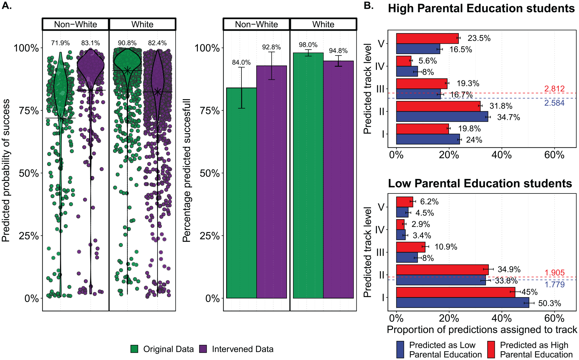
(A) Predicted probabilities (left) and outcomes (right) of successful mortgage applications for Whites and non-Whites in the data. Green values indicate predictions on the original data, whereas purple values show predictions when intervening on the race variable (i.e., changing the observed race from non-White to White and vice versa). The average predicted probability of success increases by 11.2 percent for non-Whites when changing the observed race and decreases by 8.4 percent for Whites when doing so. The predicted number of successes increases from 84 percent to 92.8 percent for non-Whites and decreases from 98 percent to 94.8 percent for Whites. (B) Predicted proportion of students in each of the five track levels for students of high parental education (top) and low parental education (bottom) when using a model fit to students of high parental education (red) or low parental education (blue). The average predicted track level is depicted using the dashed red line when predicting using the high parental education model and by the dashed blue line when predicting using the low parental education model. Confidence intervals, where present, reflect 95 percent bounds on the basis of variation in the predictive accuracy or number of predicted classes across the evaluated folds.

Instead of using predicted probabilities, it is also possible to assess the effect of a variable in terms of the actual outcome. An increase in the probability of success does not automatically reflect a similar increase in the expected number of successful applications. Probabilities will yield predictions anywhere between 0 and 1, whereas predicted outcomes will always consist of either 0 (failure) or 1 (success). The outcome-focused equivalent of the mortgage example, in which the predicted probabilities are rounded, is given on the right in Figure 4A.31 The results illustrate how intervening on the race variable would increase the share of predicted successes from 84 percent to 92.8 percent for non-Whites, while decreasing the number of predicted successes from 98 percent to 94.8 percent for Whites.³² The differences in the number of actual successes reflect that most Whites already have a high predicted probability of success before intervening on the race variable. Whether to use predicted outcomes or the underlying predicted probabilities will typically depend on the particular use case.

To illustrate the use of prediction to ask more complex interventional questions, I return to the study introduced earlier concerning teacher bias in tracking (Figure 2D). Preexisting work chose to model the outcome, track levels, as a continuous variable, allowing a straightforward interpretation of the estimated coefficients. The study illustrated earlier used an hierarchical ordered probit model leading to difficult to interpret coefficient estimates. However, by using the same interventional reasoning as outlined above, an intuitive assessment of the impact of bias features such as parental education could easily be generated (Verhagen 2021b). This reasoning was then taken a step further by assessing whether the effect of parental education could reasonably be captured by the coefficient on a dummy-coded variable, or might manifest itself through the entire model (i.e., whether students of low parental education are assessed differently on observables).

To this effect, separate models were estimated for students with low and high parental education. This led to one model fitted to students of low parental education, which could be used to make predictions for observations “as if they were low parental education students” and another model that could do the equivalent but then for high parental education students. By making predictions using both models (i.e., predicting outcomes twice) for both the low and high parental education subsets in the data, the implied difference between the two models could be assessed (Figure 4B).³³ As can be seen, high parental education students on average obtain a track level of 2.81 when assessed as high parental education students. However, when assessed as if they were low parental education students, this average track level drops by about 0.25. Conversely, low parental education students gain about 0.12 track levels when assessed as high parental education students. Determining these differences by comparing the two estimated models would not have been trivial, as multiple coefficients would have to be taken into account jointly, including random effects and the cutoff points that are estimated as part of the hierarchical ordered probit model.

Taking Stock

In this article I set out to change the underuse of prediction in the social sciences, in which prediction barely features in empirical work. This underuse occurs for the wrong reasons. Many social scientists confuse the general concept of prediction with more narrow applications, such as forecasting, or using predictive accuracy as an optimization measure. Yet prediction is a much broader and simpler analytical perspective of evaluating models in terms of their ability to accurately fit the outcome of interest. Viewed in this manner, prediction becomes a logical complement to and enrichment of the methods we have grown accustomed to using throughout the social sciences. Importantly, there is absolutely no need to sacrifice traditional modeling approaches when including prediction in empirical work, contrary to the sometimes dogmatic nature of the philosophical discussion concerning prediction and explanation. Both explanatory and predictive perspectives to analysis can and should be combined.

The benefits that prediction can bring when incorporated into the typical empirical work flow of social scientists are plenty, and this article illustrates but a few. For instance, how basic predictive consciousness can spur important debate in a research field (Figure 2A) but also how predictions allow a more detailed assessment of model fit, for example, by assessing the fit of individual predictions (Figure 2B), comparing predictive performance by subsets of the data (Figure 2C), using different models (Figure 2D), or testing our models on completely new data (Figure 2E). Prediction also provides a measure allowing social scientists to compare the fit of wildly varying methodological approaches (Figures 3A and 3B). This includes models from different paradigms, such as flexible machine learning models, which opens the way to benchmarking our models against flexible alternatives. Benchmarking provides social scientists with a way to assess whether the models we estimate have the appropriate complexity to fit the data well (Figure 3C). Finally, prediction is amenable to do-style reasoning and allows us to obtain intuitive associations between variables in nonlinear models (Figure 4A) but also to take this interventional reasoning a step further and compare how models estimated to subsets of the data differ in modeling the outcome of interest (Figure 4B).

In practice, the way in which prediction is applied fundamentally depends on the case at hand. There will be empirical settings in which interest in the ability to predict an outcome is less natural than for example in the case of the FFC.³⁴ Generally speaking, this article identifies three broad virtues: (1) using prediction as a descriptive tool to improve our understanding into the fit of a model, (2) using prediction to normatively compare different models, and (3) using prediction to help generate understanding of (complex) model behavior by interventional reasoning. These benefits help address criticisms plaguing the social sciences, such as a lack of appreciation for the real-world relevance of research findings and the use of overly simplistic models to study social life. At the same time, the cynic might question what exactly we gain from adding prediction to empirical work. Can’t we identify predictive ability by measures such as R²? Or use fit metrics such as the Akaike information criterion or Bayesian information criterion to compare models? Aren’t there specification tests to diagnose serious misspecification, and can’t we identify associations in nonlinear models, if we really tried?

The answer to all of these questions is yes, although there are various nuances that make prediction preferred. For example, existing fit metrics are in sample and can suffer from overfitting. The R² measure does not work well in every design and gives no insights into heterogeneity in a model’s fit. Nonparametric regression techniques and nonlinear models are relatively complex to estimate, and without a way to illustrate their necessity, most empirical work will remain wedded to the simple linear additive model. There are many more subtle nuances. The broader point is that predictions are disarmingly simple to understand and generate and can serve multiple goals at the same time as the examples in this article illustrate. Predictions also improve transparency by inviting a more rigorous assessment of a model’s ability to fit the data than most aggregated in-sample metrics. Requiring researchers to make predictions is a much better way to diagnose model limitations than allowing researchers to (cherry-)pick their own robustness checks or descriptives. Finally, prediction paves the way for exciting methods from other domains, such as that of machine learning, into the work flow of social scientists—methods that should become complementary to the social sciences.

Hopefully, this article can help social scientists decouple prediction from some of the field’s most intriguing and sometimes heated discussions, for example, whether explanation should imply prediction or what the role of machine learning should be in the social sciences. Although interesting, they are ultimately a distraction from what prediction as an analytical tool has to offer the social sciences. In sum, prediction’s complete lack of complexity, transparency, intuitive nature, and flexibility to build on the methods we have used for decades—rather than forcing researchers into new techniques—are all substantial assets that come at virtually no price to include into our work. In other words, prediction is truly one of those illustrious free lunch buffets that social scientists continue to ignore at their own peril.

Footnotes

Author’s Note

All code and publicly available data underlying the analyses in this article can be found at the following Zenodo repository: .

ORCID iD

Mark D. Verhagen

1

In most of the articles that mention the term predict or prediction, the authors use the commonplace, conceptual meaning term (e.g., “we predict that” or “our theory makes several predictions”). The actual process of making predictions of the outcome variable is virtually nonexistent in the literature cited. Note that the term explain or explanation features in only about 13 percent of abstracts, although this proportion likely does not reflect the proportion of work that is explanatory. Explanation is the default approach to empirical work, making it less relevant to explicitly mention the term in the abstract.

2

The single sociological article making predictions in fact generated mortality forecasts ().

3

Prediction is more commonly encountered in those social science domains that put emphasis on forecasting and projecting. Typical examples are the analysis of (financial) time series but can also include the prediction of conflicts or rare events (Cederman and Weidmann 2017), network science (Cheng et al. 2014), and demography ().

4

Whenever prediction is applied, it is usually in the form of an auxiliary regression (e.g., Heckman selection methods, two-stage least squares, or matching methods). These predictions should not be considered pure predictions, given that they are meant to support standard in-sample evaluation methods and the predictions typically are not assessed substantively.

5

Similar points have been made within the prediction versus explanation debate in sociology (e.g., Watts 2014). In this particular work, the author implies another possible reason why prediction might be underused by explanatory researchers, noting that “explanations will also become less satisfying” when forced to be predictive (p. 313). In other words, prediction might also be actively avoided by researchers as it restricts the types of explanations one can plausibly argue for.

6

Increases in data size are a key feature of the past decade, although some of the larger data sets available to social scientists need not be on par in terms of data quality (). However, for prediction small-N settings are not restrictive, as leave-one-out prediction (discussed later) still allows a predictive perspective to be pursued in such cases.

7

Note that considerable developments in the field of “explainable artificial intelligence” are advancing the interpretability of complex model spaces and even allow machine learning methods to inform functional form development in typical exponential family models as well (Lundberg and Lee 2017; Ribeiro, Singh, and Guestrin 2016; ).

8

When researchers use prediction in the context of categorical outcome variables it is more common to perform simulated prediction, where many covariates are set to their mean or median values. This approach does not actually reflect the model’s ability to approximate the outcome, as the data used need not be representative of the underlying population.

9

In the case of parametrized models without shrinkage terms, the correction term of the unexplained residuals is N − 1 N − 1 − p , where p is the number of degrees of freedom in the model. This correction term converges to one quickly for moderately sized data sets. Therefore practically, in-sample predictions might suffice for moderate N and small p. Note, however, that this correction is meant to be applied to the aggregated fit metric and not individual predictions.

10

Common examples include repeating the cross-validation routine M times: so-called repeated cross-validation. Another variant is Monte Carlo cross-validation, in which again M runs of cross-validation are done, but each run uses only a single split of the data into estimation and evaluation sets. Many of these approaches tend to converge to the same results in the limit (see for a review). For most social science applications, the number of Monte Carlo simulations M can be relatively low as the evaluation set is typically about 20 percent to 30 percent in order to accurately reflect the original data. Therefore, with M of about 100, the impact of assigning data to folds should be approximated well.

11

Fundamentally, the holdout set needs to be large enough to capture the intricacies of the original data well. Therefore, for low-dimensional data with limited variation, a small holdout set might already suffice. Conversely, high-dimensional data or clustered data might require considerably more observation in the holdout to accurately reflect the data of interest. The same rationale holds when selecting the size of the single evaluation fold in Monte Carlo cross-validation.

12

The general approach to estimating the predictive error of a model is to assess the error of all the N predictions made using cross-validation against their observed values and report the mean and standard deviation. Interestingly, cross-validation has been shown to consistently estimate the expected error of the model fit to a random data set drawn from the same underlying distribution as the training set, not the expected error of the estimated model. In addition, the approach can lead to overly narrow confidence intervals (Bates, Hastie, and Tibshirani 2021; Bengio and Grandvalet 2004). The reason is that the errors are not independent, as each observation is used in both estimation and evaluation. This problem will be minor when the impact of omitting a specific fold from the estimation process on the estimated model is small (i.e., the model is stable across the omission of folds) but can have a serious impact otherwise. Some solutions have been suggested to correctly scale the confidence intervals of predictive error for certain families of models, but research remains ongoing ().

13

All publicly available data and corresponding code underlying the reproductions are archived in a Zenodo repository, which can be accessed at the following address: .

14

Typically, the in-sample R² has been used for the purpose of evaluating explanatory power. The measure has various limitations in often encountered empirical setups, for instance when modeling ordered outcomes or estimating other nonlinear models. In those cases, information criteria are typically reported, although these tend to defy an intuitive interpretation of the models ability to fit the outcome.

15

The holdout approach was chosen because of the competitive nature of the challenge: organizers were interested in finding the best predictive model among the participants.

16

Repeated K-fold stratified cross-validation was applied, ensuring similar proportions of Whites and non-Whites in each fold, with K = 5 and M = 100. Predictive accuracy was thus estimated for a total of 500 folds.

17

The authors applied stratified Monte Carlo cross-validation with M = 250. The evaluation set represented a stratified 25 percent of the total data, ensuring similar proportions of students from each school in the estimation and evaluation sets. Predictive accuracy was thus estimated for a total of 250 folds.

18

In practice, most researchers studying tracking in the Netherlands have assumed the outcome to be continuous and estimate a simple linear model (van Leest et al. 2021). As the authors point out, this is predominantly a convenience assumption, as it yields easer-to-interpret coefficient estimates ().

19

The outcome variables were normalized such that mean differences in average wages across time would not distort the predictive performance of the model fitted in 1973.

20

Note that the data were appropriate mainly for methods exploiting some form of variable selection. Methods such as neural nets should not be recommended, as the FFC contained only 4,000 observations but more than 12,000 variables. This means that the “curse of dimensionality” would be a serious issue without variable selection or regularization techniques (). More generally, limited N might be one of the most important reasons for the lack of predictive improvement observed in the FFC.

21

Traditional information criteria and goodness-of-fit measures are often dependent on predefined functional forms to correct for the degrees of freedom in the model. When including models from different paradigms of modeling, information criteria lack comparability.

22

By default, teams submitted the predictions of a null model unless they submitted their own predictions for an outcome, which is why there is considerable density around an improvement of 0 percent, as many teams choose to focus on a select number of outcomes.

23

The matter-of-fact comment by regarding the use of random forests (a flexible machine learning technique) in their 2016 handbook Computer Age Statistical Inference is instructive here: “if the Random Forest does much better [than a traditional parametrized model], you probably have some work to do” (p. 347).

24

The models were estimated using a synthetic data set of 50,000 observations based on the observed age, work experience, and schooling in the 2018 General Social Survey. For the construction of the synthetic sample and exact functional forms underlying the three data sets, see the original study from which this example has been taken, which included a fourth functional form in which each coefficient varied by sex ().

25

The XGBoost algorithm iteratively estimates shallow decision trees to the data, giving more weight to less accurately fit observations after each iteration. Decision trees are nonlinear by design, making the XGBoost model able to fit complicated patterns while requiring no a priori specified functional form ().

26

To generate predictions, a holdout set was partitioned off equal to 20 percent of the total data set.

27

To understand the type of complexity which is missing, recent developments in the field of explainable artificial intelligence can be used (Samek et al. 2019). For the example of the Mincerian wage equation shown here, such methods accurately recovered the underlying functional forms used to generate the data ().

28

Akin to benchmarking, prediction provides a common metric for researchers to align their research efforts (Cranmer and Desmarais 2017; ). The astonishing improvements in machine learning methods can in part be attributed to such an alignment on a common goal: improving the predictive accuracy on benchmark sets.

29

Note that prediction is understood here as a tool to help interpret estimated model coefficients. Prediction does not make model results causally interpretable. Causal interpretation is encoded in the research design and model estimation, whereas prediction is a tool to assess the model after estimation ().

30

A single fivefold cross-validation run was used to generate a full set of predictions.

31

The same repeated cross-validation routine from was used for the predicted outcomes.

32

The confidence intervals show that, depending on the fold used for evaluation, the observed percentage of successes in the fold can be higher or lower than the overall mean. This follows from the fact that the data size was limited, especially for non-White applicants, leading to more variability in the baseline (). Note that the intervals should not be assessed to reflect the statistical significance of the race coefficient but rather variability in the observed preintervention probability of the White or non-White applicants in a specific fold.

33

This approach is similar in intuition to decomposition methods that decompose overall group differences in some outcome into compositional differences and effect differences (Fortin, Lemieux, and Firpo 2011). However, composition methods are often used within the typical linear additive framework, which can be restrictive. Exploiting prediction allows a wider variety of modeling approaches to be applied.

34

Examples could include stylized lab experiments or research designs such as difference-in-differences, regression discontinuity, or matching setups, as either the outcome is less intuitive or interest is fundamentally into an estimated coefficient. Nonetheless, many of the key benefits of prediction that are illustrated in this article will be equally relevant to understand the extent to which the model fits the data, irrespective of whether the outcome itself is of central substantive interest or this is less the case.

Author Biography

Mark D. Verhagen is a final-year doctoral student at Nuffield College and the Leverhulme Centre for Demographic Science, both at the University of Oxford. His work focuses on the incorporation of computational methods into traditional social science work flows. He is most interested in applying concepts and methods from computer science in order to improve functional form specification and inferential effect estimation within traditional social science domains. In addition to this, he uses computational methods to construct novel data sets. He has developed and applied methods across the domains of education, health, public policy, and law. His work has appeared in journals such as the Proceedings of the National Academy of Sciences, BMC Medicine, and PLoS ONE.

References

Athey

Susan

. 2017. “Beyond Prediction: Using Big Data for Policy Problems.” Science 355(6324):483–85.

Athey

Susan

Imbens

Guido W.

2019. “Machine Learning Methods That Economists Should Know About.” Annual Review of Economics 11:685–725.

Bates

Stephen

Hastie

Trevor

Tibshirani

Robert

. 2021. “Cross-Validation: What Does It Estimate and How Well Does It Do It?” arXiv. Retrieved February 13, 2022. https://arxiv.org/abs/2104.00673.

Bengio

Yoshua

Grandvalet

Yves

. 2004. “No Unbiased Estimator of the Variance of k-Fold Cross-Validation.” Journal of Machine Learning Research 5(September):1089–1105.

Bishop

Christopher M.

2006. Pattern Recognition and Machine Learning. New York: Springer.

Booth

Heather

. 2006. “Demographic Forecasting: 1980 to 2005 in Review.” International Journal of Forecasting 22(3):547–581.

Breen

Richard

Karlson

Kristian Bernt

Holm

Anders

. 2018. “Interpreting and Understanding Logits, Probits, and Other Nonlinear Probability Models.” Annual Review of Sociology 44:39–54.

Breiman

Leo

. 2001. “Statistical Modeling: The Two Cultures (with Comments and a Rejoinder by the Author).” Statistical Science 16(3):199–231.

Cederman

Lars-Erik

Weidmann

Nils B.

2017. “Predicting Armed Conflict: Time to Adjust Our Expectations?” Science 355(6324):474–476.

10.

Cheng

Justin

Adamic

Lada

Dow

P. Alex

Kleinberg

Jon Michael

Leskovec

Jure

. 2014. “Can Cascades Be Predicted?” Pp. 925–36 in Proceedings of the 23rd International Conference on World Wide Web. New York: Association for Computing Machinery.

11.

Cranmer

Skyler J.

Desmarais

Bruce A.

2017. “What Can We Learn from Predictive Modeling?” Political Analysis 25(2):145–66.

12.

Donoho

David

. 2017. “50 Years of Data Science.” Journal of Computational and Graphical Statistics 26(4):745–66.

13.

Efron

Bradley

Hastie

Trevor

. 2016. Computer Age Statistical Inference. Cambridge, UK: Cambridge University Press.

14.

Fortin

Nicole

Lemieux

Thomas

Firpo

Sergio

. 2011. “Decomposition Methods in Economics.” Pp. 1–102 in Handbook of Labor Economics, Vol. 4. New York: Elsevier.

15.

Freedman

David A.

1991. “Statistical Models and Shoe Leather.” Sociological Methodology 21:291–313.

16.

Greenhill

Brian

Ward

Michael D.

Sacks

Audrey

. 2011. “The Separation Plot: A New Visual Method for Evaluating the Fit of Binary Models.” American Journal of Political Science 55(4):991–1002.

17.

Grimmer

Justin

Roberts

Margaret E.

Stewart

Brandon M.

2021. “Machine Learning for Social Science: An Agnostic Approach.” Annual Review of Political Science 24:395–419.

18.

Hanmer

Michael J.

Kalkan

Kerem Ozan

. 2013. “Behind the Curve: Clarifying the Best Approach to Calculating Predicted Probabilities and Marginal Effects from Limited Dependent Variable Models.” American Journal of Political Science 57(1):263–77.

19.

Hastie

Trevor

Tibshirani

Robert

Friedman

Jerome

. 2009. The Elements of Statistical Learning: Data Mining, Inference, and Prediction. New York: Springer Science & Business Media.

20.

Heckman

James J.

Humphries

John Eric

Veramendi

Gregory

. 2018. “Returns to Education: The Causal Effects of Education on Earnings, Health, and Smoking.” Journal of Political Economy 126(S1):S197–S246.

21.

Hedström

Peter

Ylikoski

Petri

. 2010. “Causal Mechanisms in the Social Sciences.” Annual Review of Sociology 36:49–67.

22.

Hempel

Carl G.

Oppenheim

Paul

. 1948. “Studies in the Logic of Explanation.” Philosophy of Science 15(2):135–75.

23.

Hindman

Matthew

. 2015. “Building Better Models: Prediction, Replication, and Machine Learning in the Social Sciences.” Annals of the American Academy of Political and Social Science 659(1):48–62.

24.

Hofman

Jake M.

Sharma

Amit

Watts

Duncan J.

2017. “Prediction and Explanation in Social Systems.” Science 355(6324):486–88.

25.

Hofman

Jake M.

Watts

Duncan J.

Athey

Susan

Garip

Filiz

Griffiths

Thomas L.

Kleinberg

Jon

Margetts

Helen

, et al. 2021. “Integrating Explanation and Prediction in Computational Social Science.” Nature 595(7866):181–88.

26.

Kohavi

Ron

. 1995. “A Study of Cross-Validation and Bootstrap for Accuracy Estimation and Model Selection.” Pp. 1137–45 in IJCAI ’95: Proceedings of the 14th International Joint Conference on Artificial Intelligence.

27.

Lemieux

Thomas

. 2006a. “Increasing Residual Wage Inequality: Composition Effects, Noisy Data, or Rising Demand for Skill?” American Economic Review 96(3):461–98.

28.

Lemieux

Thomas

. 2006b. “The ‘Mincer Equation” Thirty Years after Schooling, Experience, and Earnings.” Pp. 127–45 in Jacob Mincer: A Pioneer of Modern Labor Economics, edited by Grossbard

New York: Springer.

29.

Lundberg

Scott M.

Lee

Su-In

. 2017. “A Unified Approach to Interpreting Model Predictions.” Pp. 4768–77 in Proceedings of the 31st International Conference on Neural Information Processing Systems. New York: Association for Computing Machinery.

30.

Miech

Richard

Pampel

Fred

Kim

Jinyoung

Rogers

Richard G.

2011. “The Enduring Association between Education and Mortality: The Role of Widening and Narrowing Disparities.” American Sociological Review 76(6):913–34.

31.

Molina

Mario

Garip

Filiz

. 2019. “Machine Learning for Sociology.” Annual Review of Sociology 45:27–45.

32.

Mullainathan

Sendhil

Spiess

Jann

. 2017. “Machine Learning: An Applied Econometric Approach.” Journal of Economic Perspectives 31(2):87–106.

33.

Munnell

Alicia H.

Tootell

Geoffrey M.B.

Browne

Lynn E.

McEneaney

James

. 1996. “Mortgage Lending in Boston: Interpreting HMDA Data.” American Economic Review 86(1):25–53.

34.

Pearl

Judea

. 2000. Causality: Models, Reasoning, and Inference. Cambridge, UK: Cambridge University Press.

35.

Rahal

Charles

Verhagen

Mark D.

Kirk

David

. 2021. “Machine Learning in the Social Sciences: Amara’s Law and an Inclination across Foster’s S-Curve?” Retrieved February 13, 2022. https://scholar.google.com/citations?view_op=view_citation&hl=en&user=9rbQDbgAAAAJ&citation_for_view=9rbQDbgAAAAJ:_FxGoFyzp5QC.

36.

Ribeiro

Marco Tulio

Singh

Sameer

Guestrin

Carlos

. 2016. “‘Why Should I Trust You?’ Explaining the Predictions of Any Classifier.” Pp. 1135–44 in Proceedings of the 22nd ACM SIGKDD International Conference on Knowledge Discovery and Data Mining. New York: Association for Computing Machinery.

37.

Rigobon

Daniel E.

Jahani

Eaman

Suhara

Yoshihiko

AlGhoneim

Khaled

Alghunaim

Abdulaziz

Pentland

Alex “Sandy”

Almaatouq

Abdullah

. 2019. “Winning Models for Grade Point Average, Grit, and Layoff in the Fragile Families Challenge.” Socius 5. Retrieved February 13, 2022. https://journals.sagepub.com/doi/full/10.1177/2378023118820418.

38.

Salganik

Matthew

. 2019. Bit by Bit: Social Research in the Digital Age. Princeton, NJ: Princeton University Press.

39.

Salganik

Matthew J.

Lundberg

Ian

Kindel

Alexander T.

Ahearn

Caitlin E.

Al-Ghoneim

Khaled

Almaatouq

Abdullah

Altschul

Drew M.

, et al. 2020. “Measuring the Predictability of Life Outcomes with a Scientific Mass Collaboration.” Proceedings of the National Academy of Sciences 117(15):8398–8403.

40.

Salganik

Matthew J.

Lundberg

Ian

Kindel

Alexander T.

McLanahan

Sara

. 2019. “Introduction to the Special Collection on the Fragile Families Challenge.” Socius 5. Retrieved February 13, 2022. https://journals.sagepub.com/doi/full/10.1177/2378023119871580.

41.

Samek

Wojciech

Montavon

Grégoire

Vedaldi

Andrea

Hansen

Lars Kai

Müller

Klaus-Robert

. 2019. Explainable AI: Interpreting, Explaining and Visualizing Deep Learning. New York: Springer Nature.

42.

Shmueli

Galit

. 2010. “To Explain or to Predict?” Statistical Science 25(3):289–310.

43.

Simonsohn

Uri

Simmons

Joseph P.

Nelson

Leif D.

2020. “Specification Curve Analysis.” Nature Human Behaviour 4(11):1208–14.

44.

Stone

Mervyn

. 1974. “Cross-Validatory Choice and Assessment of Statistical Predictions.” Journal of the Royal Statistical Society: Series B (Methodological) 36(2):111–33.

45.

van Leest

Anne

Hornstra

Lisette

van Tartwijk

Jan

van de Pol

Janneke

. 2021. “Test- or Judgement-Based School Track Recommendations: Equal Opportunities for Students with Different Socio-economic Backgrounds?” British Journal of Educational Psychology 91(1):193–216.

46.

Verhagen

Mark D.

2021a. “Identifying and Improving Functional Form Complexity: A Machine Learning Framework.” SocArXiv. Retrieved February 13, 2022. https://osf.io/preprints/socarxiv/bka76/.

47.

Verhagen

Mark D.

2021b. “To Predict and Explain. How Prediction Improves Our Understanding of Models: An Application to the Study of Teacher Bias.” SocArXiv. Retrieved February 13, 2022. https://osf.io/preprints/socarxiv/y6mnb/.

48.

Watts

Duncan J.

2014. “Common Sense and Sociological Explanations.” American Journal of Sociology 120(2):313–51.

49.

Young

Cristobal

. 2018. “Model Uncertainty and the Crisis in Science.” Socius 4. Retrieved February 13, 2022. https://journals.sagepub.com/doi/full/10.1177/2378023117737206.

50.

Yousef

Waleed A.

2020. “A Leisurely Look at Versions and Variants of the Cross Validation Estimator.” arXiv. Retrieved February 13, 2022. https://arxiv.org/abs/1907.13413.

A Pragmatist’s Guide to Using Prediction in the Social Sciences

Abstract

Keywords

A New Perspective on Prediction for the Social Sciences

Prediction Is Often Misperceived as Deterministic Forecasting

Historical Limitations Limit the Use of Prediction in the Present

Prediction Is Conflated with the Use of Convoluted Models

A Simple Definition of Prediction

In-Sample Evaluation

Cross-Validated Evaluation

External Evaluation

The Three Virtues of Prediction

Virtue 1: Prediction Provides Improved Insight into Model Fit

Virtue 2: Prediction Provides a Benchmarking Tool across Modeling Domains

Virtue 3: Prediction Can Help Generate Insights into Complicated Models

Taking Stock

Footnotes

Author’s Note

ORCID iD

1

2

3

4

5

6

7

8

9

10

11

12

13

14

15

16

17

18

19

20

21

22

23

24

25

26

27

28

29

30

31

32

33

34

Author Biography

References