
Abstract
Studying how people understand and develop concern for environmental problems is a key area of research within environmental sociology. Previous research shows that numerous social factors have measurable effects on environmental concern. However, results tend to be somewhat inconsistent across studies on this topic. One possible explanation for this is because these social factors are typically examined as independent from one another. However, these factors are interrelated in complex ways, as shown by research on the moderating effects of race and political ideology on education. Using qualitative comparative analysis (QCA), this study examines the complex ways in which previously identified social factors interact with one another to affect environmental concern. The findings suggest that aside from political ideology, all of the other factors should be understood in combination with others. The findings also suggest equifinality and asymmetry as there are multiple distinct pathways to environmental concern.
Introduction
The world currently faces numerous environmental challenges ranging from global issues such as climate change, pollution of oceans and freshwater, and overall biodiversity loss to more local issues such as toxic waste, air pollution, and food safety. Given the importance and potential dangers of these issues, sociological research on people’s attitudes toward these problems can help inform potential mitigation and policy efforts. To that end, much research in environmental sociology has examined peoples’ attitudes toward environmental issues. This research indicates that overall concern for the environment is increasing over time both within the United States and globally (Givens and Jorgenson 2013; Jones and Dunlap 1992; Marquart-Pyatt 2008). Research in this field has traditionally examined the determinants of environmental concern (Jones and Dunlap 1992; Van Liere and Dunlap 1980; Mohai and Bryant 1998). These studies often take the form of regression analyses where researchers assess how various individual-level characteristics affect concern for environmental problems. Previously identified characteristics that affect environmental concern include gender, age, urban residence, education, income, and political orientation (Clements 2012; Givens and Jorgenson 2013; Jones and Dunlap 1992; Marquart-Pyatt 2008; Samdahl and Robertson 1989; Tremblay and Dunlap 1978; Xiao and McCright 2007).
While past research in this area provides a fundamental understanding of the different drivers of environmental concern, it is not without limitations. One issue with previous research that goes back to the beginning of studies exploring environmental concern is that the results can be inconsistent (Klineberg, McKeever, and Rothenbach 1998; Van Liere and Dunlap 1981; Xiao and McCright 2007). For instance, while some studies find that affluence is associated with higher levels of environmental concern (i.e., Arcury and Christianson 1990; Meyer and Liebe 2010), others find no effect (i.e., Xiao and Dunlap 2007) or even the opposite (i.e., Pampel and Hunter 2012). Similar inconsistencies exist when examining how gender, urban residence, and race affect concern for environmental problems. In addition to issues surrounding the measurement of environmental concern (i.e., Klineberg et al. 1998), Xiao and McCright (2007) note that the inconsistencies in previous studies are partly due to methodological issues. The methodological framework used in most previous research on environmental concern, regression analysis, can be problematic if not employed correctly. One potential issue with using regression in these types of studies is that unless explicitly modeled with appropriate data, regression treats explanatory variables as independent of one another and generally assumes symmetrical effects. However, as social researchers, we know that individual-level characteristics do not exist in isolation of one another. Indeed, a core insight in sociology is the idea that social institutions are inherently interrelated with one another. Given the relative inconsistency of previous research on environmental concern and the relative methodological limitations of regression analysis, further research is needed that seeks to understand how environmental concern is affected by the complex interrelationships between individual-level characteristics identified in previous research.
In the current study, I address this by employing qualitative comparative analysis (QCA) to explore the different causal pathways associated with environmental concern. As a method, QCA seeks to bridge the divide between quantitative and qualitative research with the use of Boolean algebra to systematically examine qualitative conditions across cases (Ragin 1987). QCA has grown in popularity in recent years and is used in recent studies in environmental sociology (e.g., Grant et al. 2010; Grant, Jorgenson, and Longhofer 2018) as well as in sociology more broadly (e.g., Kalleberg and Vaisey 2005). There are a number of relative advantages to using QCA to study social relationships. Most prominently, QCA focuses on causal complexity, assumes equifinality, and uses set-theoretic logic. Causal complexity refers to the idea that explanatory effects cannot be understood in isolation to one another. Equifinality is the assumption that there are likely multiple pathways to a given outcome and that the causal effects can be either positive or negative, depending on the pathway. These set QCA apart from other methods of analysis. Finally, QCA is a configurational approach and utilizes set-theoretic logic, which is to say that it examines the degree to which individual cases fit into various sets of conditions. QCA focuses on analyzing set/subset relationships, such as the degree to which being a college graduate (subset) leads to being employed (set). Ragin (1987) and others (i.e., Fiss, Sharapov, and Cronqvist 2013) argue that relative to correlational and net-effects methods like regression, QCA can be more appropriate assessing complex social relationships. It is important to note, though, that while QCA has relative advantages to regression, it should not be seen as a replacement to regression. Indeed, Ragin (2008:190) notes that QCA should be viewed “not as a replacement for net-effects analysis, but as a complementary technique.”
This study seeks to make two contributions. The first is to advance sociological literature on environmental concern by examining the complex interrelationships between the previously identified individual-level characteristics associated with environmental concern. Given how QCA treats causal factors, it has the potential to bypass some of the methodological restrictions of regression and provide insights into the inconsistency of previous research. The second contribution is to illustrate the utility of QCA in attitudinal research more broadly, with a particular focus on the benefits of causal complexity and equifinality and their potential to contribute to theory building and refinement.
The results of the study highlight that there are multiple distinct pathways to environmental concern. Similar to previous research, being politically liberal represents an important factor for expressing concern about the environment. In fact, the results indicate that being politically liberal is sufficient on its own for achieving environmental concern. The results also highlight that other social factors beyond political ideology are important as they relate to environmental concern. However, no other social factor is sufficient on its own. Rather, they are best understood in conjunction with other factors. The results highlight equifinality and asymmetry in that some factors, such as urban/rural residence, have different effects in combination with other factors. In other words, living in urban areas is consistent with environmental concern in some pathways, but not living in an urban area is also consistent with environmental concern in other pathways. This asymmetry may partially explain why the effect of urban/rural residence has been somewhat inconsistent in previous studies. In all, the results highlight potential directions for future research and theorization on the complex interrelationships between the social bases of environmental concern.
In the next section, I discuss previous research on environmental concern. In this, I pay specific attention to the various individual-level factors that have been identified in previous research as important determinants of environmental concern. Then, I provide an overview of QCA and its fuzzy-set variant (fsQCA), with a focus on how it compares with typical regression analyses. Following a discussion on the data and how it has been calibrated, I report the results of the analysis and compare it with common regression findings. I then discuss the findings and their significance for future research on environmental concern.
Social Bases of Environmental Concern
Research on environmental concern seeks to examine the factors that can affect an individual’s attitude toward environmental problems. It has been examined as both a general attitude or value orientation as well as the intention to act in environmentally friendly ways (Fransson and Gärling 1999). Research on environmental concern is important as it allows researchers to get a better understanding of the factors that can motivate environmental action. Previous studies highlight that there are a number of factors that tend to influence an individual’s level of concern for the environment. Most research in this area has primarily focused on individuals within countries, but recent research in this field also takes the form of multilevel studies across countries. When examining the individual, most research focuses on sociodemographic factors that tend to be associated with higher levels of environmental concern. These factors include gender, age, urban residence, education, income, and political orientation (Clements 2012; Jones and Dunlap 1992; Marquart-Pyatt 2008; Samdahl and Robertson 1989; Tremblay and Dunlap 1978; Xiao and McCright 2007). Recent research also attempts to analyze how country-level factors, such as wealth or the number of environmental nongovernmental organizations, may affect levels of concern among its population (Dunlap and York 2008; Givens and Jorgenson 2011, 2013; Jorgenson and Givens 2014; Marquart-Pyatt 2007, 2012).
Gender, typically operationalized as biological sex, is perhaps the most oft-studied factor when it comes to individual-level environmental concern. In general, previous studies find that females tend to exhibit higher levels of environmental concern than males (Marquart-Pyatt 2008; McCright 2010; McCright and Dunlap 2011, 2013; McCright and Xiao 2014; Stern, Dietz, and Kalof 1993). McCright and Xiao (2014) highlight two theoretical explanations that are offered to explain this trend: gender socialization and gendered social roles. The gender socialization argument emphasizes the role of socialization during childhood. In this case, gender socialization leads to males and females developing different values from one another. Females are taught to be more altruistic than males (Stern et al. 1993). This includes, for instance, being nurturing or concerned for the well-being of others. The gender roles argument is closely tied to the gender socialization argument (gender socialization leads males and females to different social roles). This argument posits that the social roles of men and women tend to differ along the lines of labor force participation, homemaker status, and the effects of parenthood (Xiao and McCright 2012). While gender is typically seen as an important factor leading to higher levels of concern for environmental issues, findings can be inconsistent across studies. Mohai (1992) notes that while women tend to be more concerned about local environmental issues, the effect deteriorates when examining national issues. Other studies have found that males have higher levels of concern for the environment (i.e., Arcury, Scollay, and Johnson 1987; MacDonald and Hara 1994). Still other studies have found no effect of gender of environmental concern (i.e., Klineberg et al. 1998).
Age is another important factor for environmental concern. Here, the general finding is that younger people are more likely to be concerned about the environment than older people are (Clements 2012; Fransson and Gärling 1999; Klineberg et al. 1998; Van Liere and Dunlap 1980; Marquart-Pyatt 2008; Mohai and Twight 1987; Xiao and McCright 2007). Van Liere and Dunlap (1980) posit that the relationship between age and environmental concern could be due to younger people being more willing to call for substantial changes to the social order. A similar explanation, from Mohai and Twight (1987), is that the aging process tends to make individuals more conservative and cautious.
Those who live in urban areas are also thought to be more concerned about environmental issues when compared with those who live in rural areas (Arcury and Christianson 1990, 1993; Fransson and Gärling 1999; Howell and Laska 1992; Kennedy et al. 2009; Van Liere and Dunlap 1980; Tremblay and Dunlap 1978). One argument here is that individuals who reside in urban areas are more likely to experience environmental problems, such as air or water pollution (Fransson and Gärling 1999; Tremblay and Dunlap 1978). Another explanation from Tremblay and Dunlap (1978) highlights that rural residents are more likely to view the environment in terms of its utility. While earlier studies on the relationship between residency and environmental concern found significant differences between the urban and rural populations, more recent studies have found no differences between the two (Kennedy et al. 2009; Xiao and McCright 2007). Similarly, Hamilton and colleagues find that residents in rural areas tend to have the same social bases for environmental concern as the general population (Hamilton, Colocousis, and Duncan 2010; Hamilton and Lemcke-Stampone 2014).
Income and education are also often considered key components of environmental concern (Fairbrother 2013; Fransson and Gärling 1999; Van Liere and Dunlap 1980; Marquart-Pyatt 2008). Here, income and education are often hypothesized together as socioeconomic status. An influential argument here is the postmaterial values hypothesis, or the related theory of need hierarchy from Maslow (1943), which posits that higher socioeconomic status results in changing values for people (Inglehart 1995, 2000). Higher incomes allow people to place lower value on immediate material concerns and higher values on nonmaterial concerns such as environmental problems. Similarly, those with high incomes are more able to view environmental protection as an amenity they can afford compared to lower income individuals. On the other hand, it is likely that lower income individuals are more often exposed to environmental ills and that exposure leads them to be more concerned about the environment (Pampel and Hunter 2012). While some studies have found a positive effect of income on environmental concern (i.e., Franzen and Meyer 2010), it is not consistently found in studies at the individual level (e.g., Fransson and Gärling 1999; Klineberg et al. 1998; Xiao and McCright 2007), and the postmaterial values hypothesis has also been challenged in cross-national research on environmental concern (e.g., Dunlap and York 2008; Givens and Jorgenson 2011; Jorgenson and Givens 2014).
While the income component of SES is relatively inconsistent, studies on the relationship between education and environmental concern consistently show that higher levels of education are positively associated with environmental concern (Clements 2012; Franzen and Meyer 2010; Jones and Dunlap 1992; Klineberg et al. 1998; Van Liere and Dunlap 1980; Marquart-Pyatt 2007; Xiao and McCright 2007). It is argued that higher levels of education tend to expose individuals to more altruistic values and also a better understanding of problems facing society (Clements 2012). The effect of education on its own is fairly consistent across studies, but, as noted in the following, there are some interesting exceptions when the effect of political ideology is simultaneously considered.
Research on environmental attitudes also focuses on the effects of political orientation. This research consistently shows that those who identify as Democrat or politically liberal are more likely to express concern for environmental problems relative to those who identify as Republican or politically conservative (Dunlap, Xiao, and McCright 2001; Hamilton 2011; McCright and Dunlap 2013; McCright, Dunlap, and Marquart-Pyatt 2016; McCright, Xiao, and Dunlap 2014). This research mostly focuses on the ways in which the politicization of environmental problems leads to social differences on ecological issues. For instance, McCright and Dunlap (2011) explore the relationships between gender, race, and political conservatism with climate change denial. Their research indicates that conservative white males are much more likely to endorse climate change denial relative to other social groups. Similarly, other research from Hamilton (2011) suggests that the relationship between education and belief in climate change may be influenced by political orientation. Examining survey data from New Hampshire and Michigan, his research indicates that there is an interaction effect between political party identification and education level. He finds that the effect of more education for Democrats follows the traditionally expected path in that it increases the probability of seeing climate change as a threat. For Republicans, on the other hand, the effect is the opposite: More education results in viewing climate change as less of a threat.
Some Limitations of Prior Research
Despite the large of amount of research on environmental concern, results can be inconsistent from study to study. There are many potential reasons for these inconsistencies (different time periods, different levels of analysis, different populations, etc.), but two major reasons are method of analysis and measurement of environmental concern (Klineberg et al. 1998; Xiao and McCright 2007). For the latter, a major debate within this literature is on how to best measure concern for the environment. The operationalization of environmental concern is important and can affect the results in significant ways (Fransson and Gärling 1999; Klineberg et al. 1998; Xiao and McCright 2007). For instance, among other examples, Klineberg et al. (1998) highlight how measuring environmental concern as support for spending on environmental problems can accentuate the conservative/liberal divide when it comes to environmental issues because the question largely revolves around size of government issues.
While measurement of environmental concern can affect the results and contributes to inconsistency across studies, Xiao and McCright (2007) highlight that method of analysis, specifically, the misspecification of statistical models, also plays an important role. They highlight that violating assumptions of regression models, such as treating ordinal dependent variables as interval-ratio or ignoring the parallel slopes assumption in ordered logistic models, can lead to inconsistent results. In line with Xiao and McCright’s (2007) emphasis on measurement and methodology, I argue that the general focus on individual effects and assumption of symmetry is a limiting factor in understanding the social bases of environmental attitudes. For example, imagine a person who is female, older, poor, educated, and conservative. Sociologically, what sort of expectation should we have for this person? Based on previous research, being female and educated indicates that she is more likely to be concerned about the environment, but being older and conservative should have the opposite effect. Examining those factors as individual effects means we are not really sure of the complex ways in which they might affect one another, hence there is a lack of understanding on how all of these characteristics together might affect environmental attitudes.
To be sure, this is not simply an oversight of previous research. Rather, previous research has not been able to effectively examine the complex interactions between demographic factors due to the difficulty in doing so with regression analysis. When including interaction terms in regression models, it is necessary to also include all of the lower order terms (Jaccard and Turrisi 2003). For example, suppose a researcher using regression analysis wanted to examine the combined effects of gender (G), education (E), age (A), political orientation (P), and income level (I). They would begin by creating a five-way interaction term of all of those: G × E × A × P × I. In addition to the five-way interaction, they would also need to include all four-way interactions, all three-way interactions, and all two-way interactions along with all of the main effects. Attempting to (correctly) interpret such a model would be incredibly difficult, and the necessary statistical power to be able to properly estimate such a model would be substantial. There is also an increased likelihood of issues due to multicollinearity, further dissuading use of such complex interaction terms. As such, most researchers using regression avoid going beyond two-way interactions, which have relatively straightforward interpretations, and only occasionally use three-way interactions, which are difficult to interpret (Jaccard and Turrisi 2003). I propose that using QCA to explore causal complexity associated with environmental concern is one way to overcome this limitation of previous research.
Qualitative Comparative Analysis
QCA provides both systematic analysis and comparisons between cases while also maintaining a focus on cases and the qualitative differences between them (Ragin 1987, 2008). Methodologically, QCA is grounded in Mill’s method of agreement and difference (Ragin 2008). That is, studies of this type typically examine cases with similar outcomes and look at shared conditions that lead to that outcome. QCA formalizes Mill’s method of agreement and difference through the use of Boolean algebra (Ragin 1987). Boolean algebra involves creating a data set signifying the presence or absence of a condition or, similarly, whether an event occurred. In terms of notation, this is written as capital “A” for whether an event occurred or a condition is present and lower-case “a” for if it did not occur or the condition is not present within a case.
There are essentially four phases of QCA: calibration, necessity analysis, truth table construction, and sufficiency analysis. Calibration is the construction of the data set and includes determining which sets are relevant to the outcome and the degree of set membership for each case. Calibration is vitally important for the analysis. An improperly calibrated data set is likely to provide inaccurate results. Ragin and Rubinson (2009) compare calibration to research in medical studies and the natural sciences and use the example of a thermometer to show the importance of calibration. An uncalibrated thermometer can show whether something has a higher temperature relative to another object (a quantitative distinction), but it cannot indicate whether the object is hot or cold (a qualitative distinction).
There are multiple types of QCA, but the two most common are crisp-set QCA (csQCA) and fuzzy-set QCA. In csQCA, all conditions are coded as binaries and referred to as crisp sets. A case is given a value of 1 to indicate full set membership or a value of 0 if it is not fully within the set. The downside of csQCA is that much variability is lost when collapsing sets into crisp sets; the complexity of the social world is oftentimes hard to capture in solely binaries. With the inherent restrictiveness of csQCA, researchers often opt to use fsQCA instead, which allows researchers to examine both crisp sets and fuzzy sets. Fuzzy sets are more finely calibrated and capture more of the gray area for cases who are neither fully in nor fully out of a set. According to Ragin (2000:149), using fuzzy sets allows researchers to better capture the diversity of the social world because they simultaneously “refer to both differences in kind (i.e. qualitative distinctions) and to differences in degree of membership (i.e. quantitative differences) at the same time.” Fuzzy sets can be any value between 0 and 1. A value of 0 continues to represent cases that are completely out of the set, and 1 still represents cases that are fully in the set. An example of a four-value fuzzy set could be 0, .33, .67, and 1. Here, a value of .33 is given to cases that are mostly but not totally out of the set. The value of .67 is given to cases that are mostly but not completely in the set.
After proper calibration, the researcher can move forward with necessity and sufficiency analysis. Ragin (2008) recommends necessity analysis before sufficiency analysis. Necessity analysis tests for the presence of necessary conditions. A necessary condition is one that must occur for the outcome to occur. Necessity occurs when the scores of a condition are consistently higher than the scores of the outcome. That is, when a condition is necessary for an outcome to occur, the outcome is a subset of the condition. Following necessity analysis, a researcher should examine sufficiency, which explores the conditions or combination of conditions, that might be sufficient for an outcome to occur. A condition is sufficient “if by itself it can produce a certain outcome” (Ragin 1987:99). Typically, there is not one single sufficient condition for an outcome. Instead, sufficiency is usually found in a combination of various conditions, together resulting in a given outcome. These combinations of conditions are often referred to as recipes, causal pathways, or solutions. In terms of set relationships, sufficient conditions or combination of conditions are a subset of the outcome instead of the other way around (Ragin and Rubinson 2011).
A truth table is necessary to assess sufficiency. Truth tables present all logically possible combinations of conditions and whether that combination of conditions leads to the outcome. For instance, if there are two causal conditions A and B, the logical combinations could be written as AB, Ab, aB, or ab. The more causal conditions examined, the larger the truth table. The possible number of combinations = 2k, where k is the number of conditions (Ragin 2008; Rihoux and Ragin 2009). Because of the exponential nature of the conditions, Ragin and Rubinson (2009) suggest limiting the number of causal conditions to fewer than 10. Truth tables also include a consistency score for each causal combination. A consistency score essentially represents the percentage of cases of a given causal combination that achieve the outcome. For large-N QCA, Ragin (2008) recommends a consistency threshold of at least .80 (meaning that at least 80 percent of the cases in that combination result in the outcome).
Analyzing sufficiency requires truth table reduction. Truth table reduction applies Boolean algebra to find the most parsimonious solutions for achieving the designated outcome. For instance, if both solutions ABC and AbC are found to be sufficient for achieving the outcome, the minimization procedure will drop the B condition because it appears in both solutions and result in AC as the sufficient solution. The reduction procedure can produce three types of solutions: complex, intermediate, or parsimonious solutions. These differ depending on the use of remainders. Remainders are configurations that do not exist in the data. Complex solutions make no use of remainders, intermediate solutions make use of remainders that the researcher identifies as logically possible, and parsimonious solutions use all combinations regardless of whether they are possible. Regardless of the type of reduction procedure, it is only applied to the causal combinations that consistently result in the outcome. The reduced solutions (or recipes) each have a consistency score and a coverage score. Ragin (2008:44) defines coverage as assessing “the degree to which a cause or causal combination ‘accounts for’ instances of an outcome.” In other words, coverage scores assess the relative empirical importance of a given solution.
There are a number of relative advantages and disadvantages to using QCA over regression and vice versa (Fiss et al. 2013; Ragin 2008). When deciding on an analytical approach, it really depends on the type of questions being asked and the data being analyzed. A major distinction between regression and QCA is how they treat explanatory effects and causality. In QCA, the assumptions are equifinality and causal complexity. Equifinality refers to the idea that there are multiple pathways to a given outcome. Asymmetry is at play with equifinality. This means that different values of the explanatory effects can result in the outcome, not just the maximum value of the explanatory effects. In regression analyses, on the other hand, the assumptions are generally unifinality and symmetrical effects (Fiss et al. 2013; Greckhamer, Fiss, and Misangyi 2013). Unifinality assumes that the maximum value of each positive explanatory variable produces the maximum value of the dependent variable. It is possible to model explicitly to test for nonlinear and asymmetrical effects, but generally speaking, this requires more advanced models. For instance, to examine asymmetrical effects using regression requires longitudinal data to examine and differentiate the effects of increases and decreases over time (Allison 2019; York and Light 2017). As noted previously, it is also possible to get beyond the assumption of individual effects through the use of interaction terms, but these can be limited in regression (Rihoux and Ragin 2009). In all, QCA and regression have relative advantages and disadvantages. To quote Fiss et al. (2013:192), the two methods “are rather different beasts.” The preferred method depends on the research questions being examined and the data available. If a researcher is interested in exploring causal complexity, equifinality and asymmetrical effects QCA represent a potentially useful method. For exploring net effects of different causal factors, assessing statistical significance, and finding exact relationships between a cause and an effect, regression is more appropriate.
Ragin (2008) conceptualizes QCA as both an exploratory technique and complementary to regression analysis. Given this conception, particularly the emphasis on exploratory and more inductive research, I do not have any theory-driven notions of which combinations of effects will consistently lead to environmental concern. The potential combinations are numerous, and with the added assumption of asymmetry, it would be difficult to conceptualize exact expectations. That said, previous research indicates that the social bases of environmental concern are not mutually exclusive. Through the use of split samples and interaction effects, previous research examining environmental concern has examined how some factors affect one another. For instance, Hamilton (2011) uses interaction terms between education and political ideology and finds that education increases concern for Democrats but that highly educated Republicans are less likely to report concern for the environment. Similarly, McCright and Dunlap (2011, 2013) explore how gender, race, and political ideology combine to affect climate change denial, resulting in their finding of the “cool dudes” effect as they relate to conservative white males. These studies indicate that many of the factors previously treated as independent effects can moderate one another as they pertain to environmental concern. As such, further focus on how the social bases of environmental concern intersect with one another is important and may also help to explain some of the inconsistency of previous research. In all, using QCA to explore causal complexity, equifinality, and asymmetrical effects can improve our understanding of the social bases of environmental concern.
Data and Methods
There are a few different programs to consider for performing QCA. For this project, I use the fuzzy package in Stata, developed by Longest and Vaisey (2008). The fuzzy package allows the researcher to utilize a variety of statistical tests when reducing the truth table. This allows the researcher to more thoroughly test the combinations of sets prior to reduction (Longest and Vaisey 2008). In addition to other tests, this includes the ability to test whether the consistency of the combination is significantly greater than a given consistency level (say, .80), adding to the methodological rigor of QCA. As such, using Stata for QCA allows for the most robust examination and testing of causal combinations.
In this study, I examine environmental concern in the United States. I gather data from the General Social Survey (GSS) for the years 2012, 2014, and 2016 (Smith et al. 2018). After removing all instances of missing data, I end up with a sample size of 3,150 observations. I follow previous studies in this area using GSS data (Jones and Dunlap 1992; McCright et al. 2014) and operationalize concern for the environment using the variable natenvir. According to Jones and Dunlap (1992), despite the fact it is a single-item indicator, natenvir is viewed as a reliable and valid measure of environmental concern among researchers. Many other studies also use single-item indicators to operationalize environmental concern (Givens and Jorgenson 2011, 2013; Jorgenson and Givens 2014; Knight and Messer 2012). While the single-item indicators can be empirically reliable and accurate, other studies create scales from multiple indicators of pro-environmental attitudes (Fransson and Gärling 1999). While scales potentially do a better job of simultaneously capturing multiple facets of environmental concern, the benefits of single-item indicators for environmental concern are ease of interpretation and a better understanding of exactly which facet of environmental concern the results pertain to.
The variable natenvir is part of a series of questions about national spending priorities and measures respondents’ thoughts on environmental spending. The exact wording of the question is: We are faced with many problems in this country, none of which can be solved easily or inexpensively. I’m going to name some of these problems . . . and for each one I’d like you to tell me whether you think we’re spending too much money on it, too little money, or about the right amount.
During this question, respondents are asked if they think we are “spending too much, too little or about the right amount on improving and protecting the environment” (Smith et al. 2018). Given how the question is worded, a three-value fuzzy-set scale, described by Ragin (2008:31), with values of 0, .5, and 1, is an appropriate approach. Those who feel spending is too little are fully in the set of concerned for the environment and get a value of 1. I code those who responded about right at .5, highlighting their middle ground stance where they are neither fully in nor fully out of the set. I code those who responded too much as fully out of the set with a value of 0.
I include a number of causal factors in the analysis as well. Note that in regression analyses, these are referred to as variables, but in QCA, they are typically referred to as either sets or conditions. These include sex, political identification, education level, income, race, and urban residence. First, I include a crisp set of females where 1 represents females and 0 represents males. I also include a set of highly educated individuals. In this set, I use data from the survey that measures the respondent’s years of education, from the GSS variable educ. Responses range from 0 to 20 years. I transform this variable into a fuzzy set using the standard rank procedure detailed by Longest and Vaisey (2008). This procedure rank orders the variable and then produces a standardized ranking from 0 to 1. This method preserves the variation in the original variable but transforms it to make it applicable for use in fsQCA. The equation for the standardized ranking is:

I create a set of young individuals, based on the GSS variable age. To calibrate this set, I use the direct method of calibration described by Ragin (2008) and implemented in Stata with the setgen, drect command described by Longest and Vaisey (2008). Direct calibration requires choosing three anchor points representing full nonmembership in a set, a crossover point, and full membership in a set. Based on these anchor points, direct calibration uses estimates of the log odds of full membership in a set using the following formula: (degree of membership)/1 – (degree of membership). From there, the method applies a formula for standardizing the values from 0 to 1. The formula is: degree of membership = exp(log odds)/[1 + exp(log odds)] (Ragin 2008). The anchor points I use for the calibration of young individuals are 18 years old for full membership, 40 years old as the cutoff point, and 60 years old as full nonmembership. I use these values since previous research (i.e., Mohai and Twight 1987) find these ages to be associated with important changes in concern for the environment. To measure the effect of affluence, I created a set of wealthy individuals based on the GSS variable realinc. I again use the direct method of calibration for this set. The threshold for full nonmembership is $22,050, the crossover point is $39,022, and the threshold for full membership is $66,220. These values represent the 50th, 75th, and 90th percentiles, respectively.
To measure urban residence, I calibrate a set of those who live in urban areas. This comes from GSS variable size, which measures the population where the respondent lives. I again use the direct method of calibration here with anchors of 40,000 for full nonmembership, 54,000 for the crossover point, and 100,000 for full membership. These values are based on the US census definition of an urban area, which is any population over 50,000 people. I also measure political orientation, based on the GSS variable polviews. This question asks respondents to locate themselves along a seven-point scale ranging from extremely conservative to extremely liberal. Because I am interested in measuring concern for the environment (as opposed to, say, climate denial), I create the set to measure the extent to which the respondent is politically liberal. To construct a fuzzy set, I collapsed the responses into four categories. Those who responded either extremely liberal or liberal are coded as 1. Those who responded slightly liberal are coded as .67. Those who responded moderate are given a value of .33. Those who responded slightly conservative, conservative, or extremely conservative are coded as fully out of the set, 0. All sets are summarized in Table 1.
Fuzzy-Set Calibration.
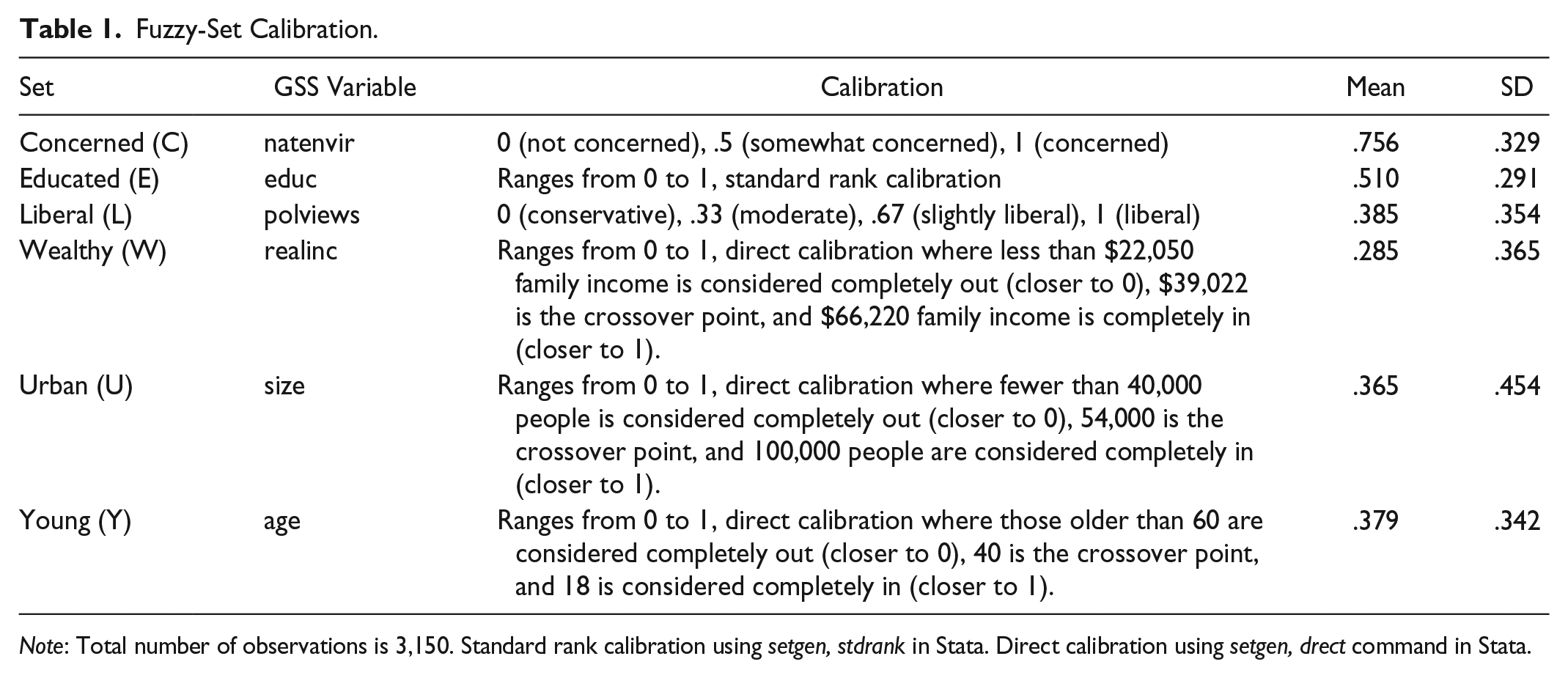
Note: Total number of observations is 3,150. Standard rank calibration using setgen, stdrank in Stata. Direct calibration using setgen, drect command in Stata.
To illustrate how using QCA differs from regression, I also estimate a regression model and present the results. I use ordered logistic regression given the dependent variable is ordinal. In the regression model, I include the same variables but not in their fuzzy set form. As such, the dependent variable ranges from a value of 1 (spend too much on protecting and improving the environment) to 3 (spend too little). Similarly, most of the independent variables are measured slightly differently as well. Sex is the exception here as I use a dummy variable where a value of 1 represents female and a value of 0 represents males (mirroring the fuzzy-set calibration described previously). For income, I log-transform (ln) realinc for ease of interpretation and because it is positively skewed. For education, I use the original values from GSS, which are simply the number of years of education. To measure liberal political orientation, I create a dummy variable for liberals using the GSS variable polviews. All respondents who indicated they are at least slightly liberal are coded 1, all others are coded 0. To measure urban residents, I again create a dummy variable from the GSS variable size. All respondents who live in areas with a population of more than 50,000 people are coded 1, and all others are coded 0. Age is measured in years and included in raw form.
Results
To set a baseline to compare our fsQCA results with, I first estimate the ordered logistic regression model of environmental concern. For ease of substantive interpretation, odds ratios are presented in the models as opposed to standard coefficients. Odds ratios are generally preferred to standard regression coefficients in logistic regression models. Odds ratios above a value of one indicate positive effects, and values below one indicate negative effects. The results of the ordered logistic regression model are reported in Table 2.
Ordered Logistic Regression of Environmental Concern.

Note: Odds ratios reported. Standard errors in parentheses.
p < .05. **p < .01. ***p < .001.
The results indicate that being female is associated with a 16.2 percent increase in the odds of thinking that we spend too little on protecting and improving the environment relative to males while holding all else constant. Age is negatively associated with environmental concern, which is consistent with some previous studies. More specifically, a one-year increase in age is associated with a 1.4 percent decrease in the odds of thinking that we spend too little on the environment while holding all else constant. Being liberal increases the odds of thinking that we spend too little on the environment by 155.4 percent relative to those who do not identify as liberals. For every additional year of education, the odds of thinking that we spend too little on the environment increases by 3.9 percent. The effect of income is negative but is nonsignificant in these models. Urban residence has a small positive effect on support for environmental spending but is also nonsignificant. The results from the regression analysis generally match up with the findings for previous studies using similar methods and measures.
For fsQCA, the first step is truth table construction. A truth table details the relationship between the outcome with all possible combinations of causal conditions, otherwise known as configurations. Here, the outcome is the set of individuals who are concerned about the environment, and the causal conditions are sets of females, wealthy individuals, highly educated individuals, liberals, and those who reside in urban areas. Truth tables typically include all cases that have a consistency score above a specified threshold, which with large-N QCA studies can be as low as .80 (Ragin 2008). Since Stata allows for more robust testing of configurations, I restrict the truth table to only those configurations that are significantly higher than .85 (p < .05). With these restrictions in place, the results yield 44 significant configurations, which are reported in Tables 3 and 4. Each row in the truth table represents a different causal combination. For instance, the first row in Table 3 consists of 53 cases that are not highly educated, not liberal, male, urban, and young. It has a consistency score of .900, meaning that 90 percent of the cases with this configuration are concerned about the environment. This same interpretation can be done for each of the rows in both truth tables.
Truth Table of Demographic Configurations.

Note: Only configurations with a consistency score significantly higher than .850 are included. Yes indicates in the set, and mo indicates out of the set. Consistency score represents proportion of cases that are in favor of more environmental spending. Observations are the number of cases that make up that configuration.
Truth Table of Demographic Configurations.

Note: Only configurations with a consistency score significantly higher than .850 are included. Yes indicates in the set, and no indicates out of the set. Consistency score represents proportion of cases that are in favor of more environmental spending. Observations are the number of cases that make up that configuration.
From the truth table, we can perform necessity analysis to examine the extent to which the outcome is a subset of the condition or set of conditions. In this case, there are no single necessary conditions or configurations that have at least a consistency level of .80. Thus, we can say that none of the causal conditions being examined are necessary for one to be concerned about the environment.
The next step is sufficiency analysis. In this case, there are no remainders because all of the possible combinations exist in the data set. As such, I simply report the complex solutions in Table 5 along with the consistency and coverage scores.
Fuzzy-Set Analysis of Environmental Concern.

Note: Total coverage = .673; total consistency = .853. Capital letters indicate to set membership, and lower case letters indicate not being in a set. E = educated; F = female; U = urban; Y = young; W = wealthy; L = liberal.
Before discussing the results of the truth table reduction, a few notes. First, each of the solutions are represented by a combination of letters representing the different sets in the analysis. In this case, “E” represents highly educated, “F” represents females, “U” represents urban residence, “Y” represents young, “W” represents wealthy, and “L” represents politically liberal. Second, while interpreting the solutions, note that the upper-case letters represent membership in a set and the lower-case letters represent nonmembership in a set. Third, in keeping with the assumptions of equifinality and causal complexity, each of the solutions must be interpreted in their entirety, not in terms of individual effects of the different conditions. Finally, each solution has an associated coverage and consistency score detailing its relative empirical relationship to the outcome.
Truth table reduction resulted in seven different solutions, or recipes, for environmental concern. This confirms my expectation that there are multiple pathways to environmental concern, indicating equifinality. The first solution consists of young educated males who live in urban areas. It has a consistency score of .912, indicating that 91 percent of the cases in this solution are concerned about the environment. The solution has a raw coverage score of .056, which indicates it only makes up around 5.6 percent of the total cases that are concerned about the environment. The second solution consists of young educated females who do not live in urban areas. It has a consistency score of .904, indicating that this solution consistently results in concern for the environment (around 90 percent of the time). This solution has a higher coverage score than the first one, representing around 11 percent of the total number of cases concerned about the environment. The third solution is comprised of young people who live in urban areas who are not wealthy. It also has a high consistency score at .894, indicating that around 89 percent of the cases with this configuration are concerned about environmental problems, and comprises 15.7 percent of the total. The fourth solution consists of young females who are not wealthy. In all, 87.6 percent of the cases in this configuration are concerned with environmental problems, comprising around 21 percent of the total. The fifth solution consists of females who live in urban areas but are not wealthy. This has the lowest consistency score at .807 but is still above Ragin’s (2008) suggestion of .8. It has a coverage score of .175, or around 17.5 percent of the total cases concerned about environmental problems. The sixth solution consists of educated females who are not wealthy. It has consistency and coverage scores of .887 and .250, respectively. The last solution is just politically liberal individuals, which has a consistency score of .901. It has a relatively large coverage score of .458, representing nearly 46 percent of the total cases who are concerned about environmental problems.
While the previous results are interesting and indicate both equifinality and causal complexity, it is important to note that QCA results can be sensitive to researcher decisions regarding calibration, consistency thresholds, and frequency thresholds (Skaaning 2011; Tanner 2014; Thiem 2014). Many researchers who use QCA point to the fact that QCA is an iterative process that requires researchers to carefully decide on their calibration procedures in regard to both theory and case knowledge (Skaaning 2011). Regardless, when using QCA, researchers must take special care to ensure that their results are relatively robust and are not simply reflections of researcher bias in calibration.
One way I deal with sensitivity issues in QCA is by making use of the tests of statistical significance built into Stata’s fuzzy program. These tests, described previously, only allow for causal combinations that are significantly greater than a .85 consistency score to be included in the truth table reduction. In addition to taking these measures to improve the robustness of the findings, I also followed recommendations from Skaaning (2011) and performed a number of additional sensitivity analyses. First, I performed fsQCA using different calibrations of education, income, and age. These are the continuous measures from the GSS that I converted into fuzzy sets using the standard rank and direct methods of calibration that were most based on researcher discretion. For an alternative education set, I used the direct method of calibration where the anchors were set at 12, 14, and 16 years of education. For alternative income and age sets, I used the standard rank method. Furthermore, following Ragin’s (2008) suggestion for large-N QCA studies, in other analyses, I excluded causal combination with fewer than 10 empirical cases from the truth table reduction procedure. The results of these sensitivity analyses remained similar to those reported here. The largest change was to the effect of political ideology. In the results presented previously, it is sufficient on its own for achieving environmental concern. However, in some of the sensitivity analyses, it is only sufficient in combination with other factors such as education or not being wealthy. I opted to present the previous results based on the fact that they resulted in the highest total coverage and consistency scores, indicating that the original calibrations carry relatively more empirical weight and are more accurate than the others.
Discussion
The findings indicate that the social bases of environmental concern are more complex than shown in previous research. In particular, the fsQCA results indicate both equifinality and causal complexity among the social bases of environmental concern. The one finding that remains completely consistent with the regression results and previous literature is that the effect of being politically liberal appears to be quite important regardless of the analytical approach taken. To some degree, this highlights the large divide that has occurred between political ideologies over the last decade-plus in the United States and shows that there is much work that needs to be done to show that environmental problems are far more than just political talking points.
The regression results indicate that being female is associated with an increase in the probability of being concerned about environmental problems relative to males. The fsQCA results show that the relationship between gender and environmental concern is somewhat more complex. In particular, they show that being female by itself is not sufficient for a person to be concerned about environmental problems. While it remains an important factor, the results here show that it should be understood in conjunction other factors such as age, education, place of residence, and wealth. Additionally, the fsQCA results highlight that the gender effect is not unidirectional. For instance, the first solution indicates that young, educated males in urban areas are consistently concerned about environmental problems. In all, though, because being female is in four of the seven reduced configurations, it is clearly an important factor that contributes to increased concern for the environment, which is in line with previous research.
Place of residence is another factor that appears to be quite important in contributing to the probability of a person being concerned about the environment. It appears in four out of seven configurations, showcasing equifinality once again. Here, living in an urban area is in three of the seven configurations and appears to matter in conjunction with gender, education, and not being wealthy. The fsQCA results also point toward causal complexity with place of residence given that not living in an urban area is a part of the second configuration along with being female, educated, and young. This is an interesting departure from the regression results. In the regression models, the urban residence dummy variable was nonsignificant, whereas it seems to play an important role in a configurational perspective. The result from the regression model is not totally unexpected as previous studies have found inconsistent results surrounding whether urban residence truly matters for environmental concern (Kennedy et al. 2009; Xiao and McCright 2007). However, when we consider the nonsignificant effect in the regression model in conjunction with the results from fsQCA, the nonsignificant effects make a bit more sense. The fsQCA results indicate that the effect of place of residence is asymmetrical. That is, it matters for environmental concern but not always in the same way. So, it is possible that place of residence is nonsignificant in the regression model because its effect actually is inconsistent and in need of further investigation. This highlights the utility of using QCA alongside regression.
Similar to gender and place of residence, age appears to be important in the fsQCA analyses, being present in four of the seven configurations. In this case, the fsQCA results are somewhat in line with the regression results in that being younger is associated with a higher probability of being concerned about the environment. Where the results differ is that being young is not sufficient by itself to being concerned about the environment, highlighting causal complexity. Education also appears to be quite important in the fsQCA analyses and is also mostly in line with previous research and the regression results. It is present in three of the seven configurations, but it is not sufficient on its own. The fsQCA results show that being highly educated in conjunction with gender, age, place of residence, or income can lead people to be more concerned about the environment.
One of the more interesting findings from these results is that income seems to matter quite a bit for environmental concern, as it is included in more than half of the solutions. It was nonsignificant in the regression models, but in conjunction with place of residence, gender, age, or education, it appears that not being wealthy can contribute to more concern for the environment. This is in contrast to theoretical propositions such as the postmaterialist value hypothesis but are consistent with the proposition that poorer people are more likely to be concerned about the environment likely because they tend to bear more of the burden of environmental harms. Overall, the fsQCA results highlight the causal complexity of the relationship between income and environmental concern.
Conclusion
In this study, I use qualitative comparative analysis to better understand the social bases of environmental concern. QCA allows researchers to examine how various causal factors come together in complex configurations, or pathways, that result in a given outcome. In contrast to regression, QCA assumes both equifinality and causal complexity. In line with this, the fsQCA results indicate that most of the social factors identified as important drivers of environmental concern in previous research are not sufficient on their own to achieve environmental concern. As such, examining their effects in isolation from other social/demographic factors is likely problematic and possibly one of the reasons for the inconsistency of past research. The one exception to this comes in the form of political ideology, which, not coincidentally, has one of the most consistent impacts on environmental concern in previous research. Additionally, I find that gender and place of residence likely have asymmetric effects on environmental concern. That is, their effects are different in combination with other factors, a finding that would be difficult to observe in a regression analysis. This research also indicates that having a high income is not a critical component of environmental concern. Instead, the results here indicate that not being wealthy is a common component of the different pathways leading to environmental concern. An overall takeaway from this study is that future research seeking to understand environmental concern would do well to more thoroughly theorize and examine the complex ways that social/demographic factors interact with one another.
While the results indicate both equifinality and causal complexity, it should be noted that this study has a number of limitations. First, given the exploratory nature of the study, I used a single item indicator of environmental concern. While I used the same variable from the GSS that is used in previous studies (e.g., Jones and Dunlap 1992; McCright et al. 2014), a common area of debate in this literature is about how to properly measure environmental concern. Indeed, it has been argued that how one measures environmental concern could have large impacts on the effects of different explanatory variables, such as income or political ideology (Klineberg et al. 1998). As such, while there are advantages to single-item indicators, future research could take heed of this to measure and calibrate environmental concern in a more comprehensive manner.
Second, for any QCA study, a major component of the research is calibrating the data set. While all of the social factors examined in this study are measured in a similar manner to previous research in their raw form, others may contend that the calibration of those factors used here should be altered in some way or another. This is entirely possible, and future research could use different calibration techniques to further refine the ways in which the fuzzy sets were defined. For example, one potentially fruitful way could be to move away from gender as a crisp set based on biological sex. Instead, following improved understandings of gender identity, it could be possibly to create a fuzzy set for gender to better understand the relationship between gender and environmental concern.
Third, QCA as a method does not rely on statistical inference, so the findings here should not be interpreted as such. Using Stata for the analyses allowed me to improve the robustness of my truth table reduction (i.e., only including combinations that were significantly higher than .85 consistency), but this is largely a methodological issue that cannot be overcome without further analysis. One potential pathway for future research on environmental concern would be to integrate the QCA results into a regression model, which has been explored in recent research in environmental sociology (i.e., Grant et al. 2018). This type of research builds on Ragin’s (2008) characterization of QCA as an exploratory and complementary technique. In this case, QCA can be used to find causal pathways that are then more rigorously examined using regression techniques that rely on statistical inference.
Finally, in this study, I analyze GSS data, which means I only examine people in the United States. Past research has shown that there are important cross-national differences in environmental concern that can be examined using data from other sources. Future research could use cross-national data and temporal QCA (which allows for the effect of time to be considered) to further examine complexity of environmental concern.