Sage Journals: Discover world-class research

Abstract

This article aims to explore the relationship between income and happiness. As shown by the Easterlin paradox, the relationship between income and happiness is not simple but indeed is rather complicated. The author used finite mixtures of regression models to analyze the data from the National Survey of Social Stratification and Social Mobility conducted in Japan and implemented computer simulations based on the results of the finite mixtures of regression models to examine how changes in social values influence the relationship between income and happiness. Analytical results revealed that people can be categorized into two latent classes: one dominated by materialistic values and the other eschewing materialistic values. Moreover, they clarified that materialistic values have ambivalent influences on individual happiness and average happiness in society. It is concluded that the diffusion of materialistic values might cause paradoxical relationships between income and happiness.

Keywords

happiness income materialistic values micro-macro link

Background

In this article, I focus on exploring the relationship between income and happiness at the individual level to clarify the types of social phenomena that can be deduced from the relationship between income and happiness. In fact, this relationship is not simple but rather is multifaceted, suggesting that social mechanisms determining individual happiness are very complicated. For example, Easterlin (1974, 1995) has shown that income and happiness do not necessarily have a positive association at the country level, even though we can easily find a positive association between income and happiness at the individual level. This paradoxical phenomenon has been called the Easterlin paradox, which compels us to reconsider the social meanings of happiness.

Of course, the validity of the Easterlin paradox on the relationship between income and happiness might be controversial. Therefore, we cannot accept the Easterlin paradox as an undoubted fact. In fact, some researchers have denied the existence of the Easterlin paradox (Diener et al. 1993; McBride 2001; Stevenson and Wolfers 2008). Nevertheless, the Easterlin paradox gives us a clue to what happiness means in modern society. Therefore, it can be said that the Easterlin paradox remains a crucial issue in the social sciences. In this article, I specify the social conditions that might generate paradoxical phenomena concerning the relationship between income and happiness and explain why and how such conditions can lead to such a paradoxical phenomenon in our society. The Easterlin paradox can then be treated as one such paradoxical phenomenon.

Previous studies have explained the Easterlin paradox using the notion of relative income or expected income. According to a theory of relative income, if individuals find that their incomes are lower than others’ income, they will feel unhappiness regardless of their absolute income (Alderson and Katz-Gerro 2016; Clark, Frijters, and Shields 2008; Ferrer-i-Carbonell 2005; Luttmer 2005; Oshio, Nozaki, and Kobayashi 2011). Similarly, if individuals find that their real incomes are lower than their expected income, they will also feel unhappiness regardless of their real income (Cummings 2019; Easterlin 2001). According to these theories, it can be predicted that increasing income inequality reduces average happiness in society as a whole even though average income in that society continues to rise (Gardarsdottir et al. 2018; Wilkinson 2005; Wilkinson and Pickett 2009). This explanation of the relationship between income and happiness seems persuasive and acceptable. However, note that there has been some doubt expressed of its validity (Firebaugh and Schroeder 2009; Kelley and Evans 2017a, 2017b; Schnittker 2008a; Wu and Li 2017).

To grasp the complicated relationship between income and happiness, I confirm not only the effects of income on happiness but also the effects of other factors on happiness. In addition, I also consider the interaction effects of income and such factors on happiness. In fact, genetic traits, demographic traits, social status, and social context have a variety of influences on individual happiness, while income is the strongest predictor of individual happiness (Diener and Seligman 2004; Schnittker 2008b). For example, previous studies clarified that age and education have a positive influence on happiness (Keyes 1998; Keyes, Shmotkin, and Ryff 2002; Yang 2008). Moreover, social institutions, social relations, and social capital are also related to individual happiness (Frey and Stutzer 2000, 2002; Hommerich and Tiefenbach 2018; Myers and Diener 1995; Ono and Lee 2013; Steel et al. 2018). Without considering their effects, therefore, one would be unable to correctly understand the complicated relationship between income and happiness.

From the perspective of the criteria for judging happiness, here, I classify people into two categories: one is the group seeking to satisfy material desires and the other seeking to satisfy nonmaterial desires (Diener, Oishi, and Lucas 2003; Ryan and Deci 2001; Waterman 1993). The group seeking to satisfy nonmaterial desires tends to judge their happiness based on various factors besides socioeconomic status (Diener and Seligman 2004; Myers and Diener 1995). I call this group the group eschewing materialistic values. On the other hand, the group seeking to satisfy material values tends to judge their happiness based on socioeconomic status. I call this group the group dominated by materialistic values. Interestingly, previous studies showed that people seeking to satisfy material values are less likely to feel happiness (Burroughs and Rindfleisch 2002; Diener and Biswas-Diener 2002; Kasser and Ahuvia 2002; Sirgy 1998; Vansteenkiste et al. 2006). In other words, seeking to satisfy material desires does not necessarily enable individuals to feel happiness but instead might well hurt individual happiness. It can then be thought that the social meanings of income and happiness differ between the two groups.

Certainly, income strongly influences individual happiness. However, its influences might not be direct but transmitted indirectly via various social values. For the group dominated by materialistic values, income has a more significant meaning, and income must thus have a strong effect on their happiness. On the other hand, for the group eschewing materialistic values, income has less significant meaning and thus a weak effect on individual happiness within this group. In this way, the effects of income on happiness are not independent from the social values that people hold. When we explore the relationship between income and happiness, therefore, we need to note the roles of various social values.

In this article, I especially focus on the role of materialistic values. Here, I define the notion of materialistic values used herein as follows: attitudes seeking socioeconomic status as the criterion of happiness and the aim of life. For individuals, such social values probably promote the likelihood of status achievement by stimulating their status aspiration. On the other hand, such high-status aspiration might reduce individual happiness by raising the expected status within individuals (Stutzer 2004). I posit that this ambivalent function of materialistic values on happiness via status aspiration plays a key role in the paradoxical changes in average happiness in developed societies.

The social meaning of income (and social statuses) constantly changes with changes in society. Accordingly, the relationship between income and happiness will vary. In particular, it is thought that materialistic values uniquely influence the relationship between income and happiness. Because materialistic values have an ambivalent function in status achievement and status satisfaction, they will greatly complicate the relationship between income and happiness. As a result, even though individuals rationally judge their happiness based on their values, the relationship between income and happiness at the macro level will show a paradoxical pattern, as with the Easterlin paradox.

Hypotheses

In this section, I present some hypotheses deduced from my theoretical explanation of the relationship between income and happiness. By checking them against empirical data, I will confirm the validity of my explanation of the relationship between income and happiness.

First, we may assume that in a society there are different groups with different perspectives on social values and happiness. One is dominated by materialistic values. They judge their happiness based on socioeconomic status (household income, occupation, employment status, educational background, etc.). The other is a group eschewing materialistic values. They judge their happiness based on social relations besides socioeconomic status (children, friends, health, etc.).

Note that the difference between the two groups is not in their levels of happiness, but in the mechanism determining individual happiness, and such a difference is generated by different social values. However, the difference in the mechanism determining happiness might result in different phenomena at the macro level, including differences in average happiness. Based on this inference, the following hypothesis was deduced:

Hypothesis 1: A population can be classified into two subpopulations. The happiness of the individuals in one subpopulation is determined based on socioeconomic status (e.g., educational level, occupation, employment, and income), and that of those in the other subpopulation is not.

Next, I assume that each subpopulation has unique traits in its value orientation and composition. As mentioned previously, members of the group dominated by materialistic values are prone to determine their happiness based on their income and social status. If they earn high incomes, they will be more likely to feel happiness. Moreover, if they attain high status, they will be more likely to feel happiness. However, as socially disadvantaged people can also have materialistic values, this does not mean that members of the group dominated by materialistic values earn high income and hold high status. Nevertheless, by setting such a criterion as the aim of life, they will make efforts to realize it and as a result tend to earn higher incomes and hold a higher status than others. Based on this inference, the following hypothesis was deduced:

Hypothesis 2a: As members of the group dominated by materialistic values make efforts to realize status attainment as the aim of life, they are more likely to earn higher incomes and attain a higher status.

Additionally, a positive correlation between income and happiness can be observed within the group dominated by materialistic values. Because members of that group are more sensitive to differences in socioeconomic statuses among them, rich individuals will feel stronger happiness than poor individuals. On the other hand, even though such a positive correlation between income and happiness is observed and the members of that group are on average advantaged in that society, the average happiness within that group will remain at a low level because their high aspiration toward status attainment raises the expected level of their status and thereby reduces their happiness. Based on this inference, the following hypothesis was deduced:

Hypothesis 2b: Within the group dominated by materialistic values, income and happiness will be positively correlated with each other, while the average level of happiness within this group will be low in comparison to that of the whole society.

Conversely, I predict that since the group eschewing materialistic values are unconcerned with socioeconomic status, they are less likely to attain high status than those in the group dominated by materialistic values. Even so, they still feel happiness as they judge their happiness independently, regardless of socioeconomic status. The following hypothesis was developed based on this inference:

Hypothesis 3a: Members of the group eschewing materialistic values are less likely to earn high incomes and attain high status, yet they feel happiness strongly.

Furthermore, the correlation between income and happiness will be weaker within the group eschewing materialistic values. Because members of that group are relatively indifferent to the differences in socioeconomic status between them, poorer individuals might feel happiness independently once their income reaches a certain level. Consequently, the average level of happiness within that group will be high. Based on this inference, the following hypothesis was deduced:

Hypothesis 3b: Within the group eschewing materialistic values, income and happiness will be weakly correlated, and the average level of happiness within that group will be high compared to that of the whole society.

If we then compare social statuses and happiness between the two groups, we will find a paradoxical relationship between income and happiness. The group dominated by materialistic values tends to be socially advantaged compared to the group eschewing materialistic values. Nevertheless, the average happiness of the group dominated by materialistic values is lower than the average happiness of the group eschewing materialistic values. Taken together, it might be predicted that socioeconomic status and happiness have a negative correlation with each other. However, the correlation between socioeconomic status and happiness still remains positive because there is a strong positive correlation between socioeconomic status and happiness for the group dominated by materialistic values, and there is a weak correlation between socioeconomic status and happiness for the group eschewing materialistic values (at least not a negative one). As the positive correlation between socioeconomic status and happiness is not offset by any negative correlation, that positive correlation between them can still remain true for society as a whole.

In this way, by assuming a micro-macro link scheme (Figure 1; Coleman 1990; Hedström 2005; Hedström and Ylikoski 2010; Raub, Buskens, and Van Assen 2011), it is possible to explain the complicated relationship between income and happiness embodied in the Easterlin paradox. At the individual level, the only assumption made is that individuals rationally judge their happiness based on their values. On the other hand, at the macro level, it is assumed that sharp changes in social values accompany rapid social changes. The diffusion of materialistic values then stimulates individuals’ aspirations toward status attainment and raises their expected socioeconomic status (this is a transition from macro to micro). Stimulating their aspirations enables them to achieve high incomes, while rising expected socioeconomic status reduces their happiness (this is a transition from micro to micro). Finally, with increases in individuals with materialistic values, average income in society rises; however, average happiness in that society declines (this is a transition from micro to macro). Nevertheless, a positive relationship between income and happiness remains at the individual level.

Figure 1.

The micro-macro link of the relationship between income and happiness.

Data and Methods

Data

To examine my hypotheses, I used data from The National Survey of Social Stratification and Social Mobility in 2015 (SSM 2015), which was conducted in Japan from February to August 2015 using a combination of personal interviews and placement methods. SSM 2015 is a national representative survey well known to Japanese sociologists (SSM Survey Management Committee 2018). The population of SSM 2015 is Japanese people aged from 20 to 80. Using a stratified random sampling method, the sample of SSM 2015 was extracted from the basic resident registers (jumin kihon daicho) administrated by each municipality of Japan. Furthermore, the number of respondents of SSM 2015 was 7,817, and the response rate was 50.1 percent. As many cases in SSM 2015 have a missing value for household income, however, I used only 5,328 of the cases for analysis.

Dependent Variable

As the dependent variable, the item for happiness from the SSM 2015 was chosen. Then all responses of the respondents to the item on happiness in SSM 2015 were collected through a paper questionnaire, not through an interview. The sentence for that item is as follows: Now, to what extent do you feel happy, where 10 is “very happy” and 0 is “very unhappy”? Therefore, the item for happiness of 2015 has an 11-point scale variable from 0 (very unhappy) to 10 (very happy), and the variable for happiness was treated as a continuous variable in the analysis.

Independent Variables

The analysis examined the effects of socioeconomic status on happiness. Therefore, I picked the variables for household income, occupation, and educational level as independent variables. Information for respondent’s household income was self-reported by each respondent through an interview. Moreover, I allotted a number of years of education to each category of educational levels: Less than high school graduate is 9, high school graduate and vocational school graduate are 12, community college graduate is 14, university graduate is 16, and graduate from graduate school is 18. I treated years of education as a continuous variable. Lastly, I categorized respondent’s occupations into five categories: upper white-collar, lower white-collar, blue-collar, job seeker, and no job. I treated them as categorical variables and made a dummy variable for each category. Here, I need to note that “no job” in SSM 2015 includes retired people, full-time homemakers, and students.

Control Variables

To estimate the effects of socioeconomic status on happiness, I controlled the effects of respondents’ demographic traits: age, gender, and family structure. I treated age as a continuous variable and input it into my analytical models as a control variable. In fact, age is known as a strong predictor for happiness (Yang 2008). Moreover, I treated gender as a categorical variable and recoded male as zero and female as one. I also treated marital status as categorical variables. I categorized respondents’ marital status into three categories: married, unmarried, and divorced/bereaved. Lastly, I treated number of children as a continuous variable and input it into my analytical models as a control variable.

Analytic Strategy 1: Finite Mixtures of Regression Models

On my hypotheses, I assumed that a whole population includes different subpopulations for feelings of happiness. To confirm this, it is necessary to identify such subpopulations in the data from the SSM 2015 and clarify differences in the mechanisms determining happiness corresponding to each subpopulation. According to my hypotheses, one subpopulation is dominated by materialistic values, whereas the other eschews such values. However, which subpopulation exceeds the other? This seems also to be an important issue because it is predicted that the balance between subpopulations influences the distribution pattern of happiness in the population. Therefore, I should estimate a composition rate for each subpopulation.

To do so, I analyzed the data from SSM 2015 using finite mixtures of regression models (Grün and Leisch 2007, 2008; Leisch 2004). As this method assumes that the whole population can be probabilistically divided into subpopulations (latent classes) and each latent class generates each distribution of the dependent variable, the distribution of the dependent variable (happiness) in that population is therefore regarded as a finite mixture distribution. Each distribution of the dependent variable by each latent class is then derived from a regression model for each latent class. Certainly, I might also use latent class analysis to extract heterogeneous subpopulations from the population, which is more familiar among sociologists. However, latent class analysis is more descriptive and less explanatory compared to finite mixtures of regression models. At least by adopting finite mixtures of regression models, I can show different mechanisms determining happiness (i.e., different regression models that predict happiness). As I focus not only on the differences in traits between subpopulations but also the differences in mechanisms determining happiness between subpopulations, I chose to adopt finite mixtures of regression models in my analysis.

Here, a finite mixture density of regression models with K latent classes is given by the following equation (Grün and Leisch 2007:4):

h (y | x, Θ) = \sum_{k = 1}^{K} π_{k} f_{k} (y | x, θ_{k}),

(1)

where Θ is the vector of all parameters for the mixture density $h$ . The dependent variable is y, and the independent variables are x. $f_{k}$ is the latent class-specific density function. The latent class-specific parameters are given by $θ_{k} = (β_{k}^{'}, ϕ_{k})$ , where $β_{k}$ is the regression coefficient and $ϕ_{k}$ is the dispersion parameter. For the latent class weights πk, it holds that:

\sum_{k = 1}^{K} π_{k} = 1 \land π_{k} > 0, \forall k .

(2)

When I analyzed the data from the SSM 2015 using finite mixtures of regression models, I estimated the parameters and coefficients using the flexmix package in Software R (Grün and Leisch 2007, 2008; Leisch 2004; R Core Team 2018).

Using finite mixtures of regression models allows us to consider the validity of my hypotheses and specify different groups in happiness feeling as latent classes in that population as well as clarify the specific mechanisms determining happiness for each latent class as a regression model. The differences between latent classes then are not in average levels of happiness but in their mechanisms determining happiness. Of course, such differences in mechanisms might generate differences in average levels of happiness among them. However, the latter differences have only secondary significance in my hypotheses, for which differences in the mechanisms determining happiness have a more significant meaning because such differences can lead to paradoxical relationships between income and happiness.

Analytic Strategy 2: Simulation Models

As SSM 2015 is a cross-sectional survey, its data do not suffice to confirm the effects of the diffusion of materialistic values on happiness unequivocally. To do so, I applied computer simulation. More specifically, I controlled the composition rates of latent classes extracted from a finite mixture of regression models counterfactually. Increasing the share of the latent class dominated by materialistic values can be looked on as modeling the diffusion of materialistic values in that society. By increasing the share of the latent class dominated by materialistic values, therefore, we can observe various changes caused by materialistic values virtually even though SSM 2015 itself is a cross-sectional survey.

First, I examined how average household income in the population changes with the diffusion of materialistic values. As it is predicted that materialistic values stimulate motivation for success, their diffusion might raise the average household income (Lyubomirsky, King, and Diener 2005; Schnittker 2008b). Next, I examined how average happiness in the population changes as materialistic values are diffused. As it is predicted that materialistic values reduce individual happiness by raising the criteria for judging happiness, their diffusion might depress the average happiness of that society (Easterlin 1995, 2001). Lastly, I compared changes in average household income and changes in average happiness with the diffusion of materialistic values and calculated changes in the correlation coefficients between household income and happiness.

To manipulate the composition rates of latent classes counterfactually, I implemented weighting resampling of the data of SSM 2015 based on the analytical results for the finite mixture of regression models. If the percentage of the latent class dominated by materialistic values is set at 0 percent and the percentage of the latent class eschewing materialistic values at 100 percent, this corresponds to the situation where materialistic values are not diffused in that society at all. Conversely, if the percentage of the latent class dominated by materialistic values is set at 100 percent and the percentage of the latent class eschewing materialistic values at 0 percent, this will model the situation where materialistic values have perfectly diffused throughout that society. In this way, I counterfactually control the degree of the diffusion of materialistic values in that society.

I used the dplyr package in R (R Core Team 2018; Wickham et al. 2016) to implement weighting resampling based on the data from SSM 2015. For concrete analysis, after implementing the computer simulations, I particularly examined 11 cases: the case of 0 percent of the materialistic class, the case of 10 percent, the case of 20 percent, and so on at increments of 10 percentage points. For each case, I randomly resampled 10,000 cases from the data of SSM 2015, referring to the composition rates set in advance and the results of the finite mixture of regression models. As a result, this computer simulation approach revealed very interesting findings on the relationships between happiness and income.

Thus, it is important to note that this method has one serious limitation. The method assumes that the correlations between variables are constant even under social change. Obviously, this assumption is unrealistic as correlations among variables are influenced by variation in social contexts: If the social context changes, correlations among variables may also change. However, using counterfactual thinking, this method can be used to estimate the effect of changes in social values themselves on happiness after controlling for the effects of changes to social contexts. Therefore, if given appropriate consideration, this limitation could instead be seen as an advantage of this method.

Analytical Results

Descriptive Statistics

Table 1 shows the descriptive statistics for the variables used in my analyses. The number of respondents is 5,328. The mean respondent age is 53.74, and the proportion of female respondents is 0.52. The mean respondent’s age seems to be a bit high, but this value reflects the sharp aging of the population observed in Japanese society and a tendency for a lower response rate in the younger generations. Therefore, this value can be accepted as reasonable. Similarly, the proportion of women in the population slightly surpasses that of men. Considering the tendency for greater female longevity, however, this value can be also accepted as reasonable. On the whole, the demographic composition of SSM 2015 does not seem seriously biased. On the other hand, the average household income is 590.7 (ten thousands of Japanese Yen). Comparing this value with 545.4, the value drawn from official statistics, this result might seem to be a bit high. The data of household income in SSM 2015 are probably biased through the exclusion of cases with missing values for household income. However, the gap between the average household income in SSM 2015 and the official statistics is not excessive, and the bias does not appear so serious. As is well known, the existence of extremely high earners tends to skew the distribution of household income from a normal distribution. Therefore, household income was converted logarithmically before being entered into my models.

Table 1.

Descriptive Statistics (Overall).

Variables	Mean	SD	Minimum	Maximum
Happiness	6.68	1.9	0	10
Age	53.74	15.3	20	80
Female (=1)	0.52
Married	0.78
Unmarried	0.11
Divorced/bereaved	0.11
N of Children	1.75	1.1	0	7
Years of education	12.88	2.33	0	18
Upper white-collar	0.17
Lower white-collar	0.22
Blue-collar	0.26
Job seeker	0.03
No job	0.32
Household income (10,000 JPY)	590.74	433.31	0	7625

Note: N = 5,328.

The mean happiness is 6.68, and the standard deviation is 1.90. As the mean of happiness exceeds 5.0, the Japanese people seem to be relatively happy. Here, we need to note the distribution profile of happiness in SSM 2015, which is shown in Figure 2. Obviously, the distribution of happiness in SSM 2015 is non-normal. Moreover, the distribution of happiness seems to have two peaks, one at approximately 8.0 and the other at approximately 5.0. If an individual’s happiness feeling is determined by only one universal mechanism, a distribution of such a shape should not appear in a society.

Figure 2.

Distribution of happiness scores.

The presence of two peaks in the distribution of happiness suggests that there are different groups with different mechanisms determining happiness in the society (Kobayashi and Hommerich 2017). One is happier (located around 8.0) than the other (located around 5.0). Here, we need to ask who the members of the two groups are and why they feel happiness (or unhappiness) because it would seem that the difference in average happiness between the two would derive from the difference in the mechanisms determining their happiness. To answer these questions, I examine the results of analyses using the finite mixtures of regression models in the next subsection.

Results of Finite Mixtures of Regression Models

First, based on the results of the finite mixtures of regression models, it is necessary to determine an adequate number of latent classes. Table 2 shows the values of information criteria for three models with one, two, and three latent classes. Comparing the models with one and two latent classes, both the Akaike Information Criterion (AIC) and Bayesian Information Criterion (BIC) for the model with one latent class exceed those for the model with two. Similarly, when comparing the models with one and three latent classes, both the AIC and BIC are greater for the former than the latter. Therefore, the model with one latent class was rejected as an adequate model well fitted to the data from SSM 2015.

Table 2.

Information Criteria for the Finite Mixtures of Regression Models.

N of Latent Classes	Log-Likelihood	df	Akaike Information Criterion	Bayesian Information Criterion
1	−10,651.6	13	21,329.15	21,417.70
2	−10,573.24	27	21,200.31	21,377.99
3	−10,526.84	41	21,135.68	21,405.49

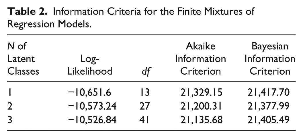
However, when comparing the models with two and three latent classes, the results for the information criteria are not consistent. AIC would indicate the model with three latent classes as more adequate, BIC the model with two latent classes. However, the third subpopulation in the model with three latent classes occupies less than 7 percent of the whole (for the detailed analytical results of the model with three latent classes, see Table A1 in the Appendix). In other words, there seems not to be substantial difference between the model with three latent classes and the model with two latent classes. Based on this result, I selected the model with two latent classes based on the principle of parsimony. Doing so allows us to interpret the results of the analyses more consistently.

Table 3 shows the results for the finite mixture of regression models (where the number of latent classes is two). First, I examine the estimated share and coefficients of the first latent class (Class 1) shown on the left side of Table 3. As the share of Class 1 is 0.802, Class 1 can be considered as constituting a majority of the Japanese population. For Class 1, years of education has a statistically significant positive effect on happiness. Highly educated individuals within Class 1 are more likely to feel happiness, while lower educated individuals within Class 1 are less likely to do so. Additionally, upper white-collar also has a statistically significant positive effect on happiness. Compared to blue-collar workers within Class 1, upper white-collar workers within Class 1 are more likely to feel happiness. In other words, members of Class 1 tend to judge their happiness with reference to their educational careers and occupational prestige. Moreover, the effect of household income is positive and has statistical significance at the p = .001 level. In short, we can consider Class 1 a group dominated by materialistic values. Interestingly, within Class 1, having no job also has a positive and statistically significant effect. This means that retired people, full-time house workers, and students are more likely to feel happiness. Probably, the positive effect of having no job reflects a negative image toward work itself, caused by the tendency for workers in Japan to have poor work-life balance (Yamaguchi 2009). On the other hand, job seekers are more less likely to feel happiness. This fact also supports the finding of previous research (Oshio et al. 2011). Additionally, as a dummy variable of marriage has a positive and statistically significant effect on happiness, the effect of marital status seemingly suggests that Japanese people tend to look at marriage as a component of social status (Sudo 2012). Lastly, among the control variables, age has a negative effect, and being a woman has a positive effect. This suggests that men are more materialistic than women on average. This fact ironically reflects on the characteristic of Japanese society as a gender gap society (Yamaguchi 2019). As women in Japan predict that they are deprived of chances in advance, they will be less likely to hold materialistic values. Meanwhile, an explanation of the effect of age on happiness is less self-evident, and I am unable to expand on these within the scope of this study. Further research would be needed to fully interpret these results.

Table 3.

Results for the Finite Mixture of Regression Models (K = 2).

	Class 1		Class 2
	Coefficients	SE	Coefficients	SE
(Intercept)	1.268**	(0.437)	8.001***	(0.582)
Age	−0.013***	(0.003)	−0.014***	(0.004)
Female	0.222**	(0.067)	0.406***	(0.102)
(Unmarried)
Married	0.943***	(0.124)	0.378	(0.215)
Divorced/bereaved	0.272	(0.150)	0.157	(0.247)
Number of children	0.067	(0.035)	0.120*	(0.050)
Years of education	0.092***	(0.016)	−0.043	(0.025)
Upper white collar	0.318**	(0.106)	−0.351*	(0.170)
Lower white collar	0.064	(0.092)	−0.256	(0.136)
(Blue collar)
No job	0.373***	(0.089)	−0.035	(0.135)
Job seeker	−0.468*	(0.204)	−0.513	(0.263)
Household income (log)	0.530***	(0.059)	0.149*	(0.059)
π	0.802		0.206

Note: N = 5,328.

p < .05. **p < .01. ***p < .001 (two-tailed tests).

Next, I examine the estimated share and coefficients of the second latent class (Class 2), shown on the right side of Table 3. As the share of Class 2 is 0.206, Class 2 can be considered a minority of the Japanese people. For Class 2, years of education has no statistically significant effect on happiness. Therefore, educational level seems to have no relevance to the feeling of happiness within Class 2. Additionally, upper white-collar has statistically significant negative effect on happiness. In other words, members of Class 2 tend not to judge their happiness with reference to their educational careers and occupational prestige. Moreover, household income has no statistically significant effect at the p = .01 level, though it does at p = .05. Therefore, we judge Class 2 to be a group eschewing materialistic values. Similar to the results for Class 1, the variable of age within Class 2 also has a significant negative effect on happiness. Moreover, gender within Class 2 also has a significant effect. This indicates the robustness of the effects of age and gender on happiness in Japanese society.

To examine the basic traits of Classes 1 and 2, I classified all respondents into two latent classes based on the estimated probability of each respondent belonging to each of the latent classes. Table 4 shows the descriptive statistics for each latent class after classifying respondents into two latent classes.

Table 4.

Descriptive Statistics (Class 1 and Class 2).

Variables	Class 1 (N = 4,271)				Class 2 (N = 1,057)				Welch’s t-Test
Variables	Mean	SD	Minimum	Maximum	Mean	SD	Minimum	Maximum	Welch’s t-Test
Happiness	6.16	1.7	0	10	8.80	0.95	5	10	−67.48***
Age	53.36	14.93	20	80	55.27	16.64	20	80	−3.42***
Female (=1)	0.51				0.59				−4.75***
Married	0.79				0.73				3.96***
Unmarried	0.11				0.12				−1.13
Divorced/bereaved	0.10				0.15				−3.97***
N of children	1.74	1.1	0	7	1.78	1.13	0	6	−0.87
Years of education	13.06	2.36	0	18	12.16	2.05	0	18	12.42***
Upper white-collar	0.20				0.07				13.54***
Lower white-collar	0.23				0.21				1.21
Blue-collar	0.25				0.31				−4.27***
No job	0.30				0.37				−4.25***
Job seeker	0.02				0.04				−2.08*
Household income (10,000 JPY)	618.29	452.01	0	7625	479.43	324.86	0	3600	11.43***

p < .05. ***p < .001 (two-tailed tests).

The average happiness in Class 1 is 6.16, which is a bit less than the average for all respondents. On the other hand, the average years of education in Class 1 is 13.06, which is greater than the average for all respondents. Furthermore, the average household income is 618.27, which is considerably higher than the average in all respondents. For socioeconomic status, members of Class 1 tend to be advantaged. They are highly educated, practice a prestigious occupation, and earn high incomes. Nevertheless, they do not feel particularly happy.

On the other hand, the average happiness in Class 2 is 8.80, which is decisively higher than the average for all respondents. It may be said that the members of Class 2 feel happiness strongly. However, the average years of education in Class 2 is 12.16, which is less than the average for all respondents. Similarly, their average household income is 479.75, which is considerably lower than the average for all respondents. At least in socioeconomic status, the members of Class 2 are not advantaged. Of course, when they judge their happiness, their income is significant for them as well. However, they seem not to have so strict a standard for their income when judging their happiness.

This shows that there are clear differences in basic traits between Classes 1 and 2. Such differences between latent classes generate seemingly paradoxical phenomena: Advantaged people tend not to feel happiness, and disadvantaged people tend to feel happiness. Moreover, these differences enable us to explain the unusual shape of a happiness distribution with two peaks. Figure 3 shows the histograms for Classes 1 and 2. The top panel of Figure 3 repeats the happiness histogram for Class 1. It clarifies that the feelings of happiness of respondents are scattered from 5 to 8 and have a single peak within that range (5–8). Similarly, the center panel shows the histogram for Class 2. It also clarifies that the happiness feelings of respondents are scattered from 8 to 10 and have a single peak within that range (8–10). Lastly, the bottom panel shows the histograms for Classes 1 and 2 together. By merging Classes 1 and 2, two peaks appear in the histogram, while each latent class has a single peak in its happiness distribution.

Figure 3.

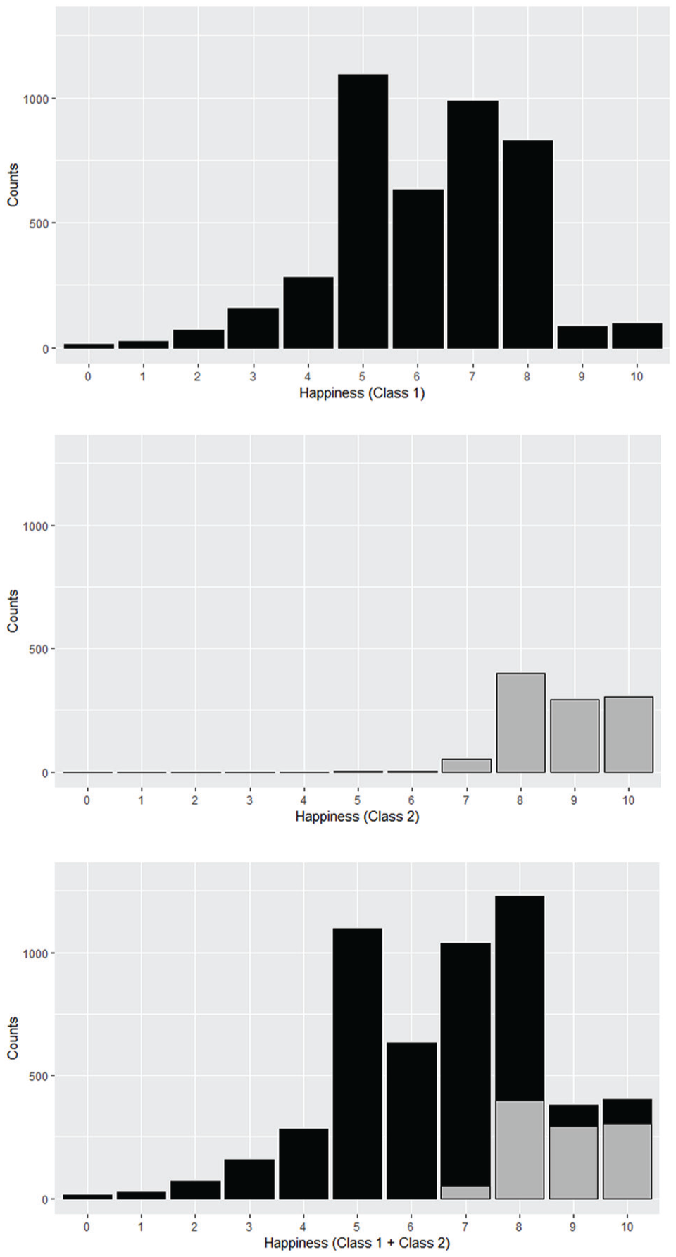
Histograms for happiness. (Top) Class 1. (Center) Class 2. (Bottom) Overall.

Results of Computer Simulation Models

In this subsection, I examine the effects of the diffusion of materialistic values on happiness. Moreover, I also examine changes in the correlation between happiness and household income with the diffusion of materialistic values. To do so, I control the share of Class 1 counterfactually to calculate average happiness, average household income, and correlation coefficients between happiness and household income. Here, I assume that if the share of Class 1 (the group dominated by materialistic values) remains at the level of 0 percent, such a state means that materialistic values do not diffuse in society. Then, if the share of Class 1 reaches the level of 100 percent, such a state means that materialistic values are perfectly diffused throughout society.

The dashed line in Figure 4 shows the changes in the average household income with the increasing share of Class 1, and the bars in Figure 4 denote 99 percent confidence intervals. Clearly, the average household income monotonically rises with increases in the share of Class 1. In other words, as materialistic values diffuse in that society, its economic level rises. This trend can be interpreted as follows: Materialistic values might stimulate individuals’ ambitions for status and economical attainment, and the individuals oriented by materialistic values to status attainment are more likely to realize economic success. As a result, diffusing materialistic values might raise the economic level of that society.

Figure 4.

Changes in average household income and average level of happiness.

Similarly, the solid line in Figure 4 shows the changes in the average feeling of happiness as the share of Class 1 increases. Clearly, the average happiness monotonically declines as the share of Class 1 increases. In other words, as materialistic values diffuse in that society, the level of subjective well-being in that society deteriorates. This trend can be interpreted as follows: Materialistic values might lead individuals to consider their socioeconomic status when judging their happiness, and the individual’s happiness is more likely to reflect the effects of social inequality. As a result, the diffusion of materialistic values might reduce the level of happiness in that society.

Figure 4 clarifies that materialistic values influence the relationship between income and happiness at the level of society. As materialistic values diffuse, people in that society gradually become richer but also gradually become unhappier. In sum, we can observe a negative relationship between income and happiness at the social level, and this relationship might appear in a society through the mediation of materialistic values. Thus, based on this fact, it might be thought that wealth and happiness are incompatible in a society. However, at the individual level, we cannot observe such a negative relationship between income and happiness. This is the most important point concerning the relationship between income and happiness.

Figure 5 shows the changes in the correlation coefficients between household income and happiness at the individual level with increases in the share of Class 1; the bars in Figure 5 demote 95 percent confidence intervals. The values of the correlation coefficient between household income and happiness are thus always positive and statistically significant. In other words, richer people are more likely to feel happiness at the individual level even though a negative correlation between household income and happiness is observed at the level of society. This result perfectly corresponds to the Easterlin paradox (Easterlin 1974, 1995, 2001). Therefore, we can assume that materialistic values play a key role in the appearance of the Easterlin paradox in our world.

Figure 5.

Changes in the correlation coefficient between household income and happiness.

Additionally, changes in the correlation coefficients between household income and happiness clarify a more interesting fact. These changes have two phases. Initially, correlation coefficients between household income and happiness weaken with increases in the share of Class 1. However, after the share of Class 1 exceeds 40 percent, the correlation coefficients between household income and happiness strengthen. In short, changes in the relationships between household income and happiness are not linear but nonlinear. Finally, the value of the correlation coefficient at 100 percent Class 1 exceeds the value of the correlation coefficient at 0 percent. Thus, people in the case of 100 percent Class 1 are more likely to connect happiness with money.

Note that as the share of Class 1 exceeds 40 percent, the relationship between household income and happiness strengthens even though people are richer and unhappier at the same time. Why does such a paradoxical phenomenon happen in the relationship between household income and happiness? The reason can be found in the difference in the variance of happiness between Class 1 and Class 2. Members of Class 1 are more sensitive to differences in socioeconomic status, and therefore Class 1 shows a wider variance in happiness than Class 2. As many members of Class 1 are unhappier and more sensitive to differences in socioeconomic status, increasing the share of Class 1 leads to strengthening the relationship between household income and happiness while at the same time people are less likely to feel happy. In this way, by considering heterogeneity within a society, the paradoxical relationship between household income and happiness can be reasonably explained.

Finally, I summarize the results of the computer simulation models. Diffusing materialistic values might bring about seemingly paradoxical relationships between income and happiness, and the Easterlin paradox can be interpreted as one such paradox. Materialistic values stimulate people’s motivation for status attainment and lead people to more success and higher incomes. Additionally, as people dominated by materialistic values are more sensitive to differences in income among people, materialistic values also enhance the positive relationship between income and happiness. At the same time, materialistic values might reduce people’s feelings of happiness by raising the criterion for happiness. Consequently, even though people are richer and the positive relationship between income and happiness becomes stronger, people will be unhappier as materialistic values diffuse through society. It can be said that materialistic values have very ambivalent meanings for people. On the other hand, we need to note some limitations of the computer simulation method adopted by this study. As mentioned previously, this method holds an unrealistic assumption that potential correlations among variables are constant even as changes to materialistic values undergo a process of diffusion. However, in reality, these potential correlations may be influenced by such changes in social contexts relating to materialistic values. Therefore, the effect of diffusing materialism on happiness should be examined using other empirical data (e.g., longitudinal data) and analytical methods (e.g., panel data analysis). Until this has been undertaken, the explanation presented in this article remains one possible explanation for the paradoxical correlation between income and happiness.

Discussion

Even though household income is a strong predictor of individual happiness, the relationship between household income and happiness is not so simple. In particular, if we focus on the micro level and the macro level at the same time, the complexity of the relationship between household income and happiness becomes more pronounced. This complicated characteristic is thought to arise from social heterogeneity. A society has groups characterized by different types of mechanisms determining individual happiness. To specify these mechanisms empirically, I analyzed the data from SSM 2015 using finite mixtures of regression models. As a result, I succeeded in extracting two latent classes from the SSM 2015 data that corresponded to my hypotheses.

Two latent classes were distinguished with respect to their criteria for happiness. One of them acted like a group dominated by materialistic values as members of that class tend to judge their happiness based on their socioeconomic status. Moreover, the other acted like a group eschewing materialistic values as members of that class tend to judge their happiness self-sufficiently rather than based on socioeconomic status. This result clearly supports Hypothesis 1 in this article. Therefore, I can argue that a society is composed of subgroups holding different value orientations for happiness.

Additionally, I implemented computer simulation models based on the data from SSM 2015 to confirm the effects of the diffusion of materialistic values on the average household income, average happiness, and correlation coefficient between household income and happiness for society as a whole. The results of computer simulation models clarified that the diffusion of materialistic values leads to rising average household income in society and declining average happiness in society as a whole. As the directions of changes in average household income and average happiness are perfectly opposite, the correlation coefficient between income and happiness will be predicted to be negative. However, this prediction did not hold.

Note that the correlation between household income and happiness at the individual level was constantly positive despite the simultaneous processes of rising household income and decreasing happiness. More interestingly, the positive correlation coefficients between household income and happiness at the individual level were enhanced once a certain share of the population was exceeded by the group dominated by materialistic values. This seemingly paradoxical phenomenon can be deduced not from differences in the average of happiness between the two latent classes but from differences in the variance of happiness between them. The group eschewing materialistic values has a small variance in happiness, and that variance was weakly explained by household income. On the other hand, the group dominated by materialistic values has a large variance in happiness, and that variance was well explained by household income. As a result, with the diffusion of materialistic values in that society, happiness will be increasingly well explained by household income.

Thus, as Hypothesis 1 was supported by the analytical results based on the data from SSM 2015, it can be concluded that a society may include different groups characterized by distinct mechanisms determining happiness. As a next step, I need to confirm whether each latent class accords with my other hypotheses: Hypotheses 2a, 2b, 3a, and 3b.

By Hypothesis 2a and 2b, I assumed that members of the group dominated by materialistic values are relatively advantaged but do not feel happiness strongly. Moreover, I also assumed that within the group dominated by materialistic values, a positive relationship between household income and happiness can be observed. The analytical results basically supported these predictions well. On the other hand, by Hypothesis 3a and 3b, I assumed that members of the group eschewing materialistic values are disadvantaged but do feel happiness strongly. In addition, I also assumed that within the group eschewing materialistic values, a positive relationship between household income and happiness cannot be observed so strongly. As a result, the social disadvantage and high happiness of the group eschewing materialistic values were supported; however, a weak positive correlation between household income and happiness was not adequately supported by the data from SSM 2015 because even in the group eschewing materialistic values, household income and happiness have a statistically significant correlation (though weaker than in the case of the other group).

In fact, the two latent classes extracted from the data from SSM 2015 have features contrasting with each other. Additionally, such features might not perfectly support my hypotheses, but they do support them in large part. Therefore, I can conclude that my hypotheses are supported by the data from SSM 2015.

Lastly, I assumed that the diffusion of materialistic values will lead to rising average household income and declining average happiness even though the relationship between household income and happiness at the micro level remains positive. The results of the computer simulation models succeeded in modeling changes in average household income, average happiness, and correlation coefficients with the diffusion of materialistic values, and they basically supported my theoretical explanation of the relationship between household income and happiness. Furthermore, these results clarified an interesting pattern of changes in the correlation coefficient between household income and happiness at the micro level. With the increased diffusion of materialistic values, the correlation coefficients did not change linearly, but nonlinearly.

Initially, as materialistic values diffuse in a society, the value of the correlation coefficient between household income and happiness sharply declines. In other words, the influence of household income on happiness seems to weaken. Such changes in the correlation coefficient were deduced from reductions in the share of happier people (the group eschewing materialistic values) and increases in the share of wealthier people (the group dominated by materialistic values). Thereafter, as materialistic values in the society subsequently diffuse further, the value of the correlation coefficient between household income and happiness sharply rises. Contrary to the first phase, the influence of household income on happiness seems to strengthen. These changes in the correlation coefficient in the second phase were deduced by increasing the share of the population more sensitive to differences in socioeconomic status (the group dominated by materialistic values).

In sum, diffusing materialistic values have opposite effects on the correlation coefficients between household income and happiness. During the first phase, as the positive effect surpasses the negative effect, the correlation coefficient between household income and happiness weakens. During the second phase, however, the relationship between the positive and negative effects becomes inverted because the group dominated by materialistic values becomes a majority in that society. As a result, the correlation coefficient between household income and happiness strengthens.

In particular, I focused on changes in the correlation coefficient during the second phase because these changes explicitly show a typical discordance between micro interactions and the macro phenomenon. During the second phase, the positive correlation between income and happiness at the micro level has strengthened. In addition, the average household income in that society consistently rises. Nevertheless, people become less likely to feel happiness. This paradoxical phenomenon cannot be explained without considering the heterogeneity of the society. At the least, the reason people are less likely to feel happiness cannot be found in changes in economic level because the average household income continues to rise. Similarly, that reason cannot be found in changes in the strength of the relationship between money and happiness because money becomes more likely to be looked on as the criterion of happiness. Only the micro-macro link scheme, which assumes changes in the share of the group dominated by materialistic values, can explain that paradoxical decline in happiness. The Easterlin paradox can probably be considered one such paradoxical phenomenon caused by the micro-macro link mechanism. According to the Easterlin paradox, average happiness at the macro level might stagnate even if the economic level at the macro level grows and the positive correlation between income and happiness remains positive at the micro level. Originally, I did not predict such paradoxical changes in the correlation between household income and happiness. Nonetheless, these findings strongly support my hypotheses. Here, we need to reconsider the social meanings of materialistic values. Materialistic values have ambivalent influences on individual happiness: While they might enhance the relationship between income and happiness, they might also reduce people’s happiness.

After all, such ambivalent characteristics of materialistic values obscure the role of money. Certainly, money always makes people happier. However, money is not an absolute criterion for happiness. If it were, we would not observe declines in average happiness with rising household income. The criterion for happiness in a society depends on the basic values of that society. By considering changes in the basic values of the society, we will correctly understand who the happiest people in that society are.

Here again, I need to point out some limitations of this study. As SSM 2015 data are cross-sectional data, I cannot examine whether these latent classes in Japan have always existed. However, when these latent classes appeared in Japan is an important problem. For example, economic stagnation during the past two decades in Japan might have had an influence on the portions of latent classes by enhancing doubt about materialistic values. Instead of declining happiness among disadvantaged people, that economic stagnation may have led to increasing the size of Class 2 in Japan. Certainly, this is only a potential explanation. As a future task in this study, I will examine the validity of that explanation by using a different data set.

Additionally, the computer simulation method adopted by this study holds an unrealistic assumption. Therefore, the explanation for the correlations between income and happiness presented in this article are not guaranteed to be generalizable. However, I believe that the findings in this article suggest new ideas for paradoxical correlations between income and happiness. In terms of future directions, I suggest using longitudinal and international comparative survey data to more accurately confirm the explanation proposed in this article.

Conclusion

The aim of this article is to explore the relationship between household income and happiness and how the relationship between them changes with social changes. As shown by the Easterlin paradox, the relationship between household income and happiness is rather complicated. Therefore, to correctly estimate the relationship between them, a detailed theoretical explanation needs to be prepared. According to the scheme of a micro-macro link, I distinguished between changes in happiness at the micro level and changes in average happiness at the macro level. By so distinguishing them, I can rationally explain the paradoxical relationship between household income and happiness.

In this article, I analyzed data from SSM 2015 to empirically confirm my theoretical explanation of the complicated relationship between household income and happiness. In addition, I applied computer simulation models based on the analytical results for finite mixtures of regression models. The analytical results of the finite mixtures of regression models thereby revealed that Japanese society is composed of two latent classes. One is the group dominated by materialistic values, the other the group eschewing materialistic values. Moreover, the results of the finite mixtures of regression models also clarified that the group dominated by materialistic values makes up a majority of Japanese society.

On the other hand, the results of the computer simulations revealed that changes in the share of the group dominated by materialistic values might generate paradoxical phenomena in the relationship between household income and happiness. The diffusion of materialistic values reduces average happiness in society as a whole even though average income rises and the positive correlation between household income and happiness is enhanced. Here, note that such paradoxical phenomena do not indicate the irrationality of individual judgement on happiness because they rationally judge their happiness based on their social values. Rather, we need to focus on the ambivalent characteristics of materialistic values.

Materialistic values raise the likelihood of status attainment by stimulating aspiration toward status attainment. It consequently raises the average income of people dominated by materialistic values. Moreover, people dominated by materialistic values are more likely to take income as a primary criterion of happiness and seek increased income. Therefore, with the diffusion of materialistic values, average income in the society rises, and the positive relationship between income and happiness is enhanced. At the same time, with the diffusion of materialistic values, it becomes difficult for individuals to meet their criterion for happiness because materialistic values raise the level of income this group expects. In this circumstance, materialistic values consequently reduce individual happiness, and we find a paradoxical relationship between income and happiness.

Footnotes

Appendix

Table A1.

Results for the Finite Mixture of Regression Models (K = 3).

	Class 1		Class 2		Class 3
	Coefficients	SE	Coefficients	SE	Coefficients	SE
(Intercept)	2.089***	(0.569)	7.679***	(0.576)	−2.204	(1.407)
Age	−0.025***	(0.004)	−0.014***	(0.003)	−0.018	(0.010)
Female	0.287**	(0.096)	0.343***	(0.085)	0.119	(0.210)
(Unmarried)
Married	1.199***	(0.174)	0.425*	(0.188)	0.310	(0.392)
Divorced/bereaved	0.543*	(0.218)	0.146	(0.218)	−0.265	(0.455)
Having children	0.074	(0.049)	0.109*	(0.043)	0.032	(0.103)
Years of education	0.126***	(0.022)	−0.025	(0.022)	0.002	(0.048)
Upper white-collar	0.407**	(0.145)	−0.239	(0.150)	0.056	(0.321)
Lower white-collar	0.206	(0.134)	−0.192	(0.118)	−0.334	(0.287)
(Blue-collar)
No job	0.553***	(0.124)	0.048	(0.118)	−0.078	(0.294)
Job seeker	−0.213	(0.273)	−0.515*	(0.240)	−0.949	(0.556)
Household income (log)	0.391***	(0.076)	0.170***	(0.058)	1.025***	(0.194)
π	0.655		0.290		0.068

Note: N = 5,328.

p < .05. **p < .01. ***p < .001 (two-tailed tests).

Acknowledgements

I would like to thank anonymous reviewers of Socius for their helpful comments. I also thank the 2015 SSM Survey Management Committee for giving me permission to use the SSM 2015.

Author’s Note

Part of the earlier idea of this study was presented in the ASA 113th Annual Meeting.

Funding

The author disclosed receipt of the following financial support for the research, authorship, and/or publication of this article: This research is supported by JSPS KAKENHI (JP25000001, 18H03647).

ORCID iD

Naoki Sudo

Author Biography

Naoki Sudo is a professor of sociology in the Department of Political Studies at Gakushuin University. He received a PhD in sociology from the University of Tokyo. He has done work in the fields of mathematical sociology. His recent studies concern the effects of social changes on social inequality, social class identification, and subjective well-being. He has published in outlets including the Social Forces, Journal of Mathematical Sociology, and Social Science Japan Journal.

References

Alderson

Arthur S.

Katz-Gerro

Tally

. 2016. “Compared to Whom? Inequality, Social Comparison, and Happiness in the United States.” Social Forces 95(1):25–54.

Burroughs

James E.

Rindfleisch

Aric

. 2002. “Materialism and Well-Being: A Conflicting Values Perspective.” Journal of Consumer Research 29(3):348–70.

Clark

Andrew E.

Frijters

Paul

Shields

Michael A.

2008. “Relative Income, Happiness, and Utility: An Explanation for the Easterlin Paradox and Other Puzzles.” Journal of Economic Literature 46(1):95–144.

Coleman

James S.

1990. Foundations of Social Theory. Cambridge, MA: Harvard University Press.

Cummings

Jason L

. 2019. “Assessing U.S. Racial and Gender Differences in Happiness, 1972–2016: An Intersectional Approach.” Journal of Happiness Studies. DOI:10.1007/s10902-019-00103-z

Diener

Biswas-Diener

Robert

. 2002. “Will Money Increase Subjective Well-Being?” Social Indicators Research 57(2):119–69.

Diener

Oishi

Shigehiro

Lucas

Richard E.

2003. “Personality, Culture, and Subjective Well-Being: Emotional and Cognitive Evaluations of Life.” Annual Review of Psychology 54(1):403–25.

Diener

Sandvik

Seidlitz

Larry

Diener

Marissa.

1993. “The Relationship between Income and Subjective Well-Being: Relative or Absolute?” Social Indicators Research 28(3):195–223.

Diener

Seligman

Martin E. P.

2004. “Beyond Money: Toward an Economy of Well-Being.” Psychological Science in the Public Interest 5(1):1–31.

10.

Easterlin

Richard A.

1974. “Does Economic Growth Improve the Human Lot? Some Empirical Eevidence.” Pp. 89–125 in Nations and Households in Economic Growth: Essays in Honor of Moses Abramovitz, edited by David

P. A.

Reder

M. W.

New York: Academic Press.

11.

Easterlin

Richard A.

1995. “Will Raising the Incomes of All Increase the Happiness of All?” Journal of Economic Behavior & Organization 27(1):35–47.

12.

Easterlin

Richard. A.

2001. “Income and Happiness: Towards a Unified Theory.” The Economic Journal 111(473):465–84.

13.

Ferrer-i-Carbonell

Ada

. 2005. “Income and Well-Being: An Empirical Analysis of the Comparison Income Effect.” Journal of Public Economics 89(5-6):997–1019.

14.

Firebaugh

Glenn

Schroeder

Matthew B.

2009. “Does Your Neighbor’s Income Affect Your Happiness?” American Journal of Sociology 115(3):805–31.

15.

Frey

Bruno S.

Stutzer

Alois

. 2000. “Happiness, Economy and Institutions.” The Economic Journal 110(466):918–38.

16.

Frey

Bruno S.

Stutzer

Alois

. 2002. “What Can Economists Learn from Happiness Research?” Journal of Economic Literature 40(2):402–35.

17.

Gardarsdottir

Ragna B.

Bond

Rod

Vilhjalmsdottir

Amdis

Dittmar

Helga

. 2018. “Shifts in Subjective Well-Being of Different Status Groups: A Longitudinal Case-Study during Declining Income Inequality.” Research in Social Stratification and Mobility 54:46–55.

18.

Grün

Bettina

Leisch

Friedrich

. 2007. “Fitting Finite Mixtures of Generalized Linear Regressions in R.” Computational Statistics and Data Analysis 51(11):5247–52.

19.

Grün

Bettina

Leisch

Friedrich

. 2008. “FlexMix Version 2: Finite Mixtures with Concomitant Variables and Varying and Constant Parameters.” Journal of Statistical Software 28(4):1–35.

20.

Hedström

Peter

2005. Dissecting the Social: On the Principles of Analytical Sociology. Cambridge: Cambridge University Press.

21.

Hedström

Peter

Ylikoski

Petri

. 2010. “Causal Mechanisms in the Social Sciences.” Annual Review of Sociology 36:49–67.

22.

Hommerich

Carola

Tiefenbach

Tim

. 2018. “Analyzing the Relationship between Social Capital and Subjective Well-Being: The Mediating Role of Social Affiliation.” Journal of Happiness Studies 19(4):1091–114.

23.

Kasser

Tim

Ahuvia

Aaron

. 2002. “Materialistic Values and Well-Being in Business Students.” European Journal of Social Psychology 32(1):137–46.

24.

Kelley

Jonathan

Evans

M. D. R.

2017a. “The New Income Inequality and Well-Being Paradigm: Inequality Has No Effect on Happiness in Rich Nations and Normal Times, Varied Effects in Extraordinary Circumstances, Increases Happiness in Poor Nations, and Interacts with Individuals’ Perceptions, Attitudes, Politics, and Expectations for the Future.” Social Science Research 62:39–74.

25.

Kelley

Jonathan

Evans

M. D. R.

2017b. “Societal Inequality and Individual Subjective Well-Being: Results from 68 Societies and Over 200,000 Individuals, 1981–2008.” Social Science Research 62:1–23.

26.

Keyes

Corey L. M.

1998. “Social Well-Being.” Social Psychology Quarterly 61(2):121–40.

27.

Keyes

Corey L.

Shmotkin

Dov

Ryff

Carol D.

2002. “Optimizing Well-Being: The Empirical Encounter of Two Traditions.” Journal of Personality and Social Psychology 82(6):1007–22.

28.

Kobayashi

Jun

Hommerich

Carola

. 2017. “Are Happiness and Unhappiness Two Sides of the Same Coin?” Sociological Theory and Methods 32(1):49–63.

29.

Leisch

Friedrich

. 2004. “Flexmix: A General Framework for Finite Mixture Models and Latent Class Regression in R.” Journal of Statistical Software 11(8):1–18.

30.

Luttmer

Erzo F.

2005. “Neighbors as Negatives: Relative Earnings and Well-Being.” The Quarterly Journal of Economics 120(3):963–1002.

31.

Lyubomirsky

Sonja

King

Laura

Diener

. 2005. “The Benefits of Frequent Positive Affect: Does Happiness Lead to Success?” Psychological Bulletin 131(6):803–55.

32.

McBride

Michael

. 2001. “Relative-Income Effects on Subjective Well-Being in the Cross-section.” Journal of Economic Behavior & Organization 45(3):251–78.

33.

Myers

David G.

Diener

Ed.

1995. “Who Is Happy?” Psychological Science 6(1):10–19.

34.

Ono

Hiroshi

Lee

Kristen Schultz

. 2013. “Welfare States and the Redistribution of Happiness.” Social Forces 92(2):789–814.

35.

Oshio

Takashi

Nozaki

Kayo

Kobayashi

Miki

. 2011. “Relative Income and Happiness in Asia: Evidence from Nationwide Surveys in China, Japan, and Korea.” Social Indicators Research 104(3):351–67.

36.

R Core Team. 2018. R: A Language and Environment for Statistical Computing. Vienna: R Foundation for Statistical Computing. https://www.R-project.orgRcoreteam.

37.

Raub

Werner

Buskens

Vincent

Van Assen

Marcel A.

2011. “Micro-Macro Links and Microfoundations in Sociology.” The Journal of Mathematical Sociology 35(1–3):1–25.

38.

Ryan

Richard M.

Deci

Ed L.

2001. “On Happiness and Human Potentials: A Review of Research on Hedonic and Eudaimonic Well-Being.” Annual Review of Psychology 52(1):141–66.

39.

Schnittker

Jason

. 2008a. “Diagnosing Our National Disease: Trends in Income and Happiness, 1973 to 2004.” Social Psychology Quarterly 71(3):257–80.

40.

Schnittker

Jason

. 2008b. “Happiness and Success: Genes, Families, and the Psychological Effects of Socioeconomic Position and Social Support.” American Journal of Sociology 114(S1):S233–59.

41.

Sirgy

M. Joseph

. 1998. “Materialism and Quality of Life.” Social Indicators Research 43(3):227–60.

42.

SSM Survey Management Committee. 2018. “2015 SSM Reports.” http://www.l.u-tokyo.ac.jp/2015SSM-PJ/report.html

43.

Steel

Piers

Taras

Vasyl

Uggerslev

Krista

Bosco

Frank

. 2018. “The Happy Culture: A Theoretical, Meta-analytic, and Empirical Review of the Relationship between Culture and Wealth and Subjective Well-Being.” Personality and Social Psychology Review 22(2):128–69.

44.

Stevenson

Betsey

Wolfers

Justin

. 2008. Economic Growth and Subjective Well-Being: Reassessing the Easterlin Paradox (No. w14282). Cambridge, MA: National Bureau of Economic Research.

45.

Stutzer

Alois

. 2004. “The Role of Income Aspirations in Individual Happiness.” Journal of Economic Behavior & Organization 54(1):89–109.

46.

Sudo

Naoki

. 2012. “Mikon-sha no Kaiso-ishiki” [Social Class Identification of the Unmarried]. Sociological Theory and Methods 27(2):225–42. In Japanese.

47.

Vansteenkiste

Maarten

Duriez

Bart

Simons

Joke

Soenens

Bart

. 2006. “Materialistic Values and Well-Being among Business Students: Further Evidence of Their Detrimental Effect.” Journal of Applied Social Psychology 36(12):2892–908.

48.

Waterman

Alan S.

1993. “Two Conceptions of Happiness: Contrasts of Personal Expressiveness (Eudaimonia) and Hedonic Enjoyment.” Journal of Personality and Social Psychology 64(4):678–91.

49.

Wickham

Hadley

Francois

Romain

Henry

Lionel

Müller

Kirill

. 2016. dplyr: A Grammar of Data Manipulation (R package version 0.5. 0). Vienna: R Foundation for Statistical Computing.

50.

Wilkinson

Richard G.

2005. The Impact of Inequality: How to Make Sick Societies Healthier. New York: The New Press.

51.

Wilkinson

Richard G.

Pickett

Kate

. 2009. The Spirit Level. Why More Equal Societies Almost Always Do Better. London: Allen Lane.

52.

Xiaogang

Jun

. 2017. “Income Inequality, Economic Growth, and Subjective Well-Being: Evidence from China.” Research in Social Stratification and Mobility 52:49–58.

53.

Yamaguchi

Kazuo

. 2009. Waku raifu baransu: Jissho to seisaku teigen [Work Life Balance: Demonstration and Policy Proposals]. Tokyo: Nihon Keizai Shinbunsha. In Japanese.

54.

Yamaguchi

Kazuo

. 2019. Gender Inequalities in Japanese Workplace and Employment: Theories and Empirical Evidence. Singapore: Springer.

55.

Yang

. 2008. “Social Inequalities in Happiness in the United States, 1972 to 2004: An Age-Period-Cohort Analysis.” American Sociological Review 73(2):204–26.

Why Do Advantaged People Feel Unhappy? Effects of Materialistic Values on Subjective Well-Being

Abstract

Keywords

Background

Hypotheses

Data and Methods

Data

Dependent Variable

Independent Variables

Control Variables

Analytic Strategy 1: Finite Mixtures of Regression Models

Analytic Strategy 2: Simulation Models

Analytical Results

Descriptive Statistics

Results of Finite Mixtures of Regression Models

Results of Computer Simulation Models

Discussion

Conclusion

Footnotes

Appendix

Acknowledgements

Author’s Note

Funding

ORCID iD

Author Biography

References