Sage Journals: Discover world-class research

Abstract

Predicting longitudinal outcomes from thousands of variables across multiple waves provides impressive opportunities to identify variables of importance, but what is the most efficient way to carry out such analyses on hundreds or thousands of variables? As part of the Fragile Families Challenge, a series of analyses were conducted that aimed at identifying a few reliable, important variables, primarily with machine-learning approaches given minimal oversight. Using generalized boosted models, random forests, and elastic net regression models, these analyses identified a consistent set of psychological and socioeconomic factors that yielded strong prediction scores in generalized linear models. These results demonstrate that relatively simple models fitted to the Fragile Families data can generate predictions that perform close to state-of-the-art predictive models.

Keywords

socioeconomic disadvantage cognitive ability variable selection prediction family background

Decades of research has been devoted to understanding the contributions of socioeconomic background and cognitive ability to future success and hardship (for a review see Strenze 2007). Although there is immense difficulty in disentangling these two factors, ability and background, from each other, both are nonetheless powerful and reliable predictors of future success.

The Fragile Families Challenge (FFC) was a competition that used the longitudinal Fragile Families and Child Wellbeing Study in a unique way. After the sixth wave of data collection, challenge entrants were given access to data on six major life outcomes from the most recent wave (see “Methods” for a complete description), but this was only a portion of the entire data set. Entrants’ goal was to train the highest scoring (i.e., most accurate) predictive model using these incomplete data and the full range of data from all five previous waves. The data available for prediction included a wide range of socioeconomic and psychological variables reported by mothers, fathers, teachers, and the focal children themselves (Salganik, Lundberg, Kindel, and McLanahan 2019).

A major goal of the FFC was to identify variables that are already collected, infrequently used by researchers, yet could be leveraged to improve prediction of a variety of life outcomes for disadvantaged families. Neither cognitive abilities nor socioeconomic circumstances could be argued to be unmeasured or even understudied. However, given that a vast body of research exists to support the relevance of these factors, ability and background were likely to be implicated in any model with a high prediction score. Given what is already known about ability and background, what can an isolated individual researcher or citizen-scientist with limited resources, time, and direction, glean from a data set of thousands of variables?

I chose to approach the questions posed by the FFC from a practicality perspective. Many questions posed by the FFC are methodological: with thousands of variables to choose from, how does one begin to choose which to analyze? In many disciplines, one would first formulate a hypothesis and choose variables on the basis of this hypothesis. However, a key goal of the FFC was to maximize the predictive power of one’s model, and preselecting a comparatively small number of variables is not necessarily the best way to accomplish this, given that another goal of the FFC was to identify variables that are already collected but are not frequently used by researchers. The variables one might hypothesize as being involved in these outcomes are, as mentioned, possibly overstudied. One way to protect against researcher bias and save resources is to use automated, machine-learning techniques to identify key variables and build strong predictive models (Witten et al. 2016).

The goals of my analyses were to build models with good predictive strength, with interpretable parameters, using methods that are straightforward and accessible. To these ends, my analytic strategy was as follows (see also Figure 1). First, I blindly identified informative variables using generalized boosting, a machine-learning technique. Second, informed by these variables, I added others I thought could be related. Different machine-learning techniques are better at different tasks, and I wished to leverage multiple such techniques where it would be most appropriate to benefit from the strengths of each technique. Thus, I then applied elastic net and generalized linear regression techniques to my variables subset to determine predictive strength of the models as well as which individual variables were robustly related to different outcomes. I made minimal adjustments to how functions were run, and except where noted, all functions were run with their default values.

Figure 1.

Analytic approach. m refers to the number of columns in the full training data set; in the early steps of the process, the number of columns available was pared down to a smaller set for which missing values were imputed and ultimately analyzed in regression models.

Methods and Results

Data Processing

The Fragile Families training data set contained 12,943 columns, which included variables one would not expect to be related to the six outcome variables: material hardship and eviction (outcomes relating to a focal child’s household), layoffs and job training (concerning the focal child’s primary caregiver), and grade point average (GPA) and grit (outcomes for the focal child himself or herself) (for more details on the key variables, see Salganik et al. 2019). For example, the training data set included administrative variables and flags, which are effectively noise. I wished to remove these variables to reduce false positives and speed up processing time, as machine-learning and imputation techniques can be processor intensive. However, eliminating all the unrelated variables in advance of analyses is a substantial task for a small team, not to mention a single person.

The first step was setting all values in the data set less than zero to “NA.” I then chose to rely on near-zero variance filtering to remove problematic variables. Near-zero variance is a symptom of variables that have only one unique value or a very large ratio of the frequencies of the most common and second most common values. Variables were selected using the nearZeroVar function from package caret (Williams et al. 2017) (using the default settings). No distinction was made between numeric and categorical variables during this process, as the training data set did not contain this information; variable meaning was investigated later, at the imputation stage. The near-zero variance filtering method is liberal: 4,402 of 12,943 columns were excluded. However, the generalized boosted models (GBMs) could not run without near zero-variance filtering. Apart from these changes, I did not take any further steps to clean the data, allowing the variable selection via machine learning to do all additional filtering.

Generalized Boosted Modeling

Generalized boosted modeling is a powerful machine-learning technique that fits a series of decision trees and optimizes a loss function over each iteration of the tree (Ridgeway 2007). In other words, each progressive tree attempts to better model outcomes that have been mismodeled by the previous trees. The final model is composed of many trees, each weak on its own, but that together usually display very good predictive performance. Because there are many trees and the individual contributions are difficult to describe, the model is known as a “black box”: the process that takes input and produces an output is not usually known and not easily interpreted. Nevertheless, GBMs do output the “relative influence” of variables, which is based on the number of times a variable is selected to split a tree (Elith, Leathwick, and Hastie 2008).

Generalized boosted modeling was chosen for the first stage of variable selection because it is effective at identifying important variables from a large set of inputs and can also handle missing values. However, because many low-variance variables were omitted and GBMs produce black-box models, the GBMs were solely used as starting points to identify variables of interest and build interpretable models.

For binary outcome variables (eviction, layoffs, and job training), I used the AdaBoost method (a variant for dichotomous outcomes only) in my GBMs (Mayr et al. 2014). For nonbinary outcome variables (GPA and grit), I used a Gaussian link. For material hardship, a scale that can be reformatted to count up to 11, I used a Poisson link after converting each variable to a discrete value. A Poisson link was used because material hardship is a discreet count variable heavily right skewed (Joe and Zhu 2005), with 807 of 1,459 data points indicating that an individual experienced zero material hardship. Subsequent sensitivity analyses using GBMs of material hardship with a Gaussian link identified the same variables of importance.

The variables selected by each GBM are presented with estimates of influence in Table 1. The GBMs did not identify many variables, and those they did identify were similar. The Woodcock-Johnson (WJ) applied problems test was found to be important in all GBMs, and the Peabody Picture Vocabulary test was selected for all outcomes except job training. These two cognitive testing variables were the only variables selected, except in the material hardship and eviction models. In these two models, economic variables were also selected, including several related to phone service, food costs, and other bills. Although these parental variables were predictive of children’s outcomes, some of the variables concerning the children, such as test scores, could also be predictive of outcomes for the parents.

Table 1.

Relative Influence of Variables in Each Gradient Boosted Model.

Variable	Year	GPA	Grit	MH	Eviction	Layoff	JT
Woodcock-Johnson applied problems test	9	91.51	37.83	37.22	84.97	97.51	100
Peabody Picture Vocabulary test	9	8.49	62.17	0.90	3.42	2.49
Did not pay full bills	9			25.64
Number of days without phone service	9			20.20	8.22
Number of days without phone service	5			10.14
Telephone service disconnected	9			2.15
Telephone service disconnected	5			0.82
Did not pay full rent or mortgage	5			0.93
Approximate monthly amount received in food stamps	9			1.01
Did not pay full rent or mortgage	9				1.03
Reason welfare office cut aid	5				2.35
Ate less than felt should, due to money	3				0.98

Note: Relative influence indicates the proportion of grown trees in the boosted model that branch using a given variable. Influence is standardized out of 100. The Peabody Picture Vocabulary test is the sum of influences from both the percentile rank and age equivalency scores. GPA = grade point average; JT = job training; MH = material hardship.

Manually Selecting Related Variables

I wanted to include additional variables in further steps of the analysis, though I wished to add variables that tapped into the same or similar underlying phenomena as were implicated by the GBMs. Thus, I searched the study documentation for and selected additional cognitive and socioeconomic variables of interest from both the focal child and parents’ data. Because a goal of the FFC was to identify underused variables, and the earlier in life meaningful variables can be identified the more useful they might be for future study design, I searched all waves for relevant variables to add.

The inability to pay bills and buy food is likely linked to income, so for subsequent stages, I added several numeric income variables (3 for the mother, 2 for the father), as well as other variables linked to risky employment and behavior, including whether mothers worked more than one job at a time, worked off the books, or were booked or charged by law enforcement. On the other hand, the WJ and Peabody Picture Vocabulary tests identified by the GBMs were two of several psychological measures of ability, though in general, there were many fewer cognitive and academic performance variables in the entire Fragile Families data set than socioeconomic variables. I found and included all additional test scores of cognition in both the focal children (digit span test and WJ passage comprehension test from children age 9) and their parents (Wechsler Adult Intelligence Scale–Revised [WAIS-R] similarities subtest for both mothers and fathers). I also included teacher assessments of performance from year 5 (rates in language and literacy, science and social studies, and math and whether the child fell behind in school).

Multiple Imputation

Missing values in the variables from the birth through year 9 training set posed a problem for prediction because I did not know which individuals in the holdout data set would have missing data, and many modeling packages can fit models only to complete data sets. It was too costly to impute all missing values in the entire data set, so I chose to take a conservative approach and imputed all missing values among the variables of interest I had selected after searching the study documentation. Some variables were added at this stage primarily for the purposes of assisting with imputation; these included sex, city weight, and whether the mother was interviewed at the 1-year follow-up.

I used multivariate imputation by chained equations (Azur et al. 2011) for multiple imputation. In keeping with my goal of maintaining a straightforward, unsupervised analysis approach, I used the random-forests method to impute all variables of interest. Random forests is a broadly applicable machine-learning method that is conceptually similar to GBMs (Ogutu, Piepho, and Schulz-Streeck 2011). In a multiple imputation context, random forests have the advantage of requiring neither user supervision nor a priori assumptions about the relationships among variables. City weight and all six outcome variables were included in the data set, and thus they informed the imputation of the other variables, but their values were not used in subsequent analyses. Ten data sets, using a maximum of 50 iterations per imputation, were imputed. Additional information about imputation is available in the supporting online materials.

Elastic Net Regression Models

With these data, I wished to fit models that would produce predictions for the holdout dataset, in addition to interpretable regression coefficients. I chose to model these data with elastic net regression models (ENRMs), a method reliant on shrinking regression coefficients. Prediction models based on one sample will tend to overestimate variable coefficients, resulting in poorer prediction accuracy in another sample. One method for combating this is coefficient shrinkage, which reduces the strength of coefficients to improve predication accuracy.

ENRMs are one such method. ENRMs combine least absolute shrinkage and selection operator and ridge regression (Zou and Hastie 2005) and optimize model prediction accuracy via cross-validation. ENRMs produce a range of coefficient values, though ENRMs are able to shrink coefficients to zero, thus entirely removing them from the equation. The best coefficients are typically found using internal cross-validation procedures (Friedman, Hastie, and Tibshirani 2010). Cross-validation models are generated using the same training data set, and as with information criteria, cross-validation methods can be overly optimistic under such circumstances, and thus, a slightly more conservative choice of coefficients is suggested. For this reason, the coefficients found 1 standard error from the values that minimize cross-validation prediction error are often used in subsequent out-of-sample prediction. For each outcome variable, I used the same type of link function as was used in the GBMs (e.g., AdaBoost converted to a binomial distribution).

Despite having many fewer variables to choose from, several ENRMs selected a wider array of variables than the GBMs (Table 2). For example, GBMs of grit indicated that only the WJ applied problems test and the Peabody Picture Vocabulary test were predictive of these outcomes, but the ENRM of grit eliminated many fewer variables during the variable reduction process, ultimately leaving 14 variables in the model. Every variable was selected by at least one model, while year 9 WJ passage comprehension test rank and failing to pay bills in year 9 were selected predictors in all six models.

Table 2.

Elastic Net Coefficients for Regression Models of All Outcome Variables.

Variable	Year	Participant	GPA	Grit	MH	Layoff	Eviction	JT
Focal child’s gender	0	Focal	0.027	−0.021	0.007	0.012		−0.008
Mother interviewed at 1-year follow-up	1	Mother	0.014		0.011			0.006
Child fell behind in school	5	Focal	0.010		−0.077	−0.079
Rate in language and literacy	5	Focal			−0.006	−0.011
Rate in science and social studies	5	Focal			−0.042
Rate in math	5	Focal			−0.003	−0.021
Ever been booked or charged	3	Mother			−0.019	−0.175
Range of household income previous year	3	Mother			−0.004		−0.025	0.012
Worked more than one job at a time	3	Mother	0.008		−0.017			−0.020
Number of regular jobs held over two or more weeks	3	Mother	−0.052	−0.006	0.036			0.125
Worked off the books	3	Mother	0.000		−0.043	−0.010
Range of total household income	3	Mother	0.008		−0.000			0.028
Range of household income from previous year	3	Father	0.000		−0.021		−0.013
Household income (with imputation)	3	Father	0.032	−0.005	−0.058		−0.040	0.022
WAIS-R similarities subtest score	3	Father		−0.010	−0.022	−0.012
WAIS-R similarities subtest score	3	Mother	0.004			0.033		0.032
Household income (with imputation)	1	Mother	0.063	−0.008	−0.103		−0.041	0.096
Household income (with imputation)	0	Father	0.009	−0.016	−0.028	−0.032	−0.010
Digit span test: % rank	9	Focal	0.009		−0.008			0.073
Peabody Picture Vocabulary test: % rank	9	Focal	0.074	−0.025	−0.032	−0.002		0.015
WJ passage comprehension test: % rank	9	Focal	0.004	−0.018	−0.009	−0.034	−0.030	0.008
WJ applied problems test: % rank	9	Focal	0.074	−0.006	−0.004
Have failed to pay all bills	9	Mother	0.009	0.001	−0.170	−0.056	−0.016	−0.064
Number of days without phone service	9	Mother			0.035	0.034
Number of days without phone service	5	Mother			0.015	0.031	0.000
Have failed to pay full rent or mortgage	5	Mother		0.008	−0.104	−0.106	−0.015
Telephone service has been disconnected	9	Mother		0.004	−0.107	−0.303	−0.023	−0.039
Telephone service has been disconnected	5	Mother	0.018		−0.101	−0.128	−0.016
Have failed to pay full rent or mortgage	9	Mother	0.026	0.020	−0.080	−0.271		−0.037
Reason why welfare office cut off aid	5	Mother			0.017
Amount received in food stamps in the last month	9	Mother	0.004		0.011	0.000		−0.000
Ate less than felt should, due to money	3	Focal		−0.007		0.034		0.014

Note: Estimates shown are standardized regression coefficients. Where no value is given, this indicates that the estimate for this coefficient was shrunken to zero. Elastic net models do not produce standard errors, because the estimates are biased. GPA = grade point average; JT = job training; MH = material hardship; WAIS-R = Wechsler Adult Intelligence Scale–Revised.

Generalized Linear Regression Models

In addition to submitting predictions of the holdout data from the ENRMs, I also wished to compare the ENRMs’ prediction performance to general or generalized linear models (GLMs), in order to benchmark ENRM application to these sorts of data against more widely used methods. For each outcome, an ENRM and a GLM (reduced model; Table 3) were fitted to the training data using the variables selected by the ENRM; an additional GLM (full model; Table S2) was fit for each outcome using all variables available for selection by the ENRMs. Again, the same error distributions were used as in the GBMs and ENRMs.

Table 3.

Linear and Generalized Linear Regression Models for All Six Outcomes, with Reduced Predictor Variables.

Variable	Year	Participant	GPA	Grit	MH	Layoff	Eviction	JT
Focal child’s gender	0	Focal	0.049 (0.002)	−0.038 (0.004)	0.039 (0.026)†	−0.029 (0.022)†		−0.069 (0.020)
Mother interviewed at 1-year follow-up	1	Mother	0.034 (0.007)		0.049 (0.036)†			0.059 (0.028)*
Child fell behind in school	5	Focal	0.023 (0.005)		−0.095 (0.018)	0.023 (0.021)†
Rate in language and literacy	5	Focal			−0.013 (0.030)†	0.031 (0.026)†
Rate in science and social studies	5	Focal			−0.058 (0.028)*
Rate in math	5	Focal			0.003 (0.031) †	−0.019 (0.025)†
Ever been booked or charged	3	Mother			−0.025 (0.021)†	0.085 (0.024)
Range of household income previous year	3	Mother			−0.031 (0.032)†		−0.016 (0.042)†	0.047 (0.020)*
Worked more than one job at a time	3	Mother	0.020 (0.006)		−0.036 (0.024)†			−0.052 (0.019)*
Number of regular jobs held over two or more weeks	3	Mother	−0.069 (0.006)	−0.021 (0.004)	0.055 (0.026)*			0.219 (0.021)
Worked off the books	3	Mother	0.011 (0.005)*		−0.071 (0.022)*	−0.051 (0.021)*
Range of total household income	3	Mother	0.006 (0.007)†		0.019 (0.032)†			0.047 (0.023)*
Range of household income from previous year	3	Father	−0.009 (0.006)†		−0.025 (0.033)†		−0.118 (0.045)*
Household income (with imputation)	3	Father	0.037 (0.008)	−0.010 (0.005)†	−0.073 (0.037)†		0.075 (0.049)†	0.037 (0.024)†
WAIS-R similarities subtest score	3	Father		−0.019 (0.004)	−0.048 (0.027)†	−0.014 (0.024)†
WAIS-R similarities subtest score	3	Mother	0.011 (0.006)†			−0.065 (0.023)*		0.051 (0.021)*
Household income (with imputation)	1	Mother	0.076 (0.008)	−0.010 (0.005)*	−0.157 (0.039)		0.184 (0.049)	0.176 (0.026)
Household income (with imputation)	0	Father	0.004 (0.007)†	−0.029 (0.005)	−0.024 (0.035)†	−0.100 (0.025)	−0.182 (0.051)
Digit span test: % rank	9	Focal	0.015 (0.006)*		−0.029 (0.028)†			0.143 (0.021)
Peabody Picture Vocabulary test: % rank	9	Focal	0.097 (0.007)	−0.033 (0.005)	−0.044 (0.035)†	0.021 (0.029)†		0.011 (0.025)†
WJ passage comprehension test: % rank	9	Focal	−0.014 (0.008)†	−0.020 (0.005)	−0.011 (0.036)†	−0.131 (0.028)	−0.129 (0.039)	0.018 (0.025)†
WJ applied problems test: % rank	9	Focal	0.092 (0.007)	−0.012 (0.005)*	0.010 (0.034)†
Have failed to pay all bills	9	Mother	0.016 (0.006)†	0.007 (0.004)†	−0.206 (0.026)	−0.094 (0.023)	−0.173 (0.036)	−0.124 (0.021)
Number of days without phone service	9	Mother			0.058 (0.023)*	−0.007 (0.023)
Number of days without phone service	5	Mother			0.031 (0.024)†	0.049 (0.021)†	0.102 (0.036)*
Have failed to pay full rent or mortgage	5	Mother		0.018 (0.004)	−0.115 (0.021)	−0.073 (0.021)	−0.186 (0.029)
Telephone service has been disconnected	9	Mother		0.013 (0.004)*	−0.111 (0.024)	−0.076 (0.023)	−0.529 (0.031)	−0.088 (0.021)
Telephone service has been disconnected	5	Mother	0.027 (0.005)		−0.106 (0.023)	−0.054 (0.022)*	−0.169 (0.032)
Have failed to pay full rent or mortgage	9	Mother	0.036 (0.006)	0.030 (0.004)	−0.087 (0.023)	0.043 (0.023)†		−0.060 (0.020)*
Reason why welfare office cut off aid	5	Mother			0.032 (0.023)†
Amount received in food stamps in the last month	9	Mother	0.020 (0.006)		0.033 (0.025)†	−0.021 (0.022)†		−0.036 (0.020)†
Ate less than felt should, due to money	3	Focal		−0.018 (0.004)		0.023 (0.022)†		0.055 (0.019)*

Note: Estimates shown are standardized regression coefficients. All coefficients are significant at p < .001 except as indicated. Italic type indicates that the elastic net regression model estimated the opposite sign for this coefficient. GPA = grade point average; JT = job training; MH = material hardship; WAIS-R = Wechsler Adult Intelligence Scale–Revised.

p < .05. †p > .05.

Holdout Predictions

When using multiply imputed data sets for prediction, it is typical to use modeling software that takes into account the variability in imputations and produces estimates as a distribution or interval, not a single point. Because the FFC required point estimates to score submissions, I created a different predicted value for each participant within each imputed data set, then aggregated across imputations. To reach a final prediction for each participant, I took the mean of all predictions, including the binary outcome variables. Predictions were evaluated by the organizational FFC team and based on the mean squared error, using holdout data that were never shown to challenge participants.

The prediction scores of the ENRMs were strongest for GPA, material hardship, and job training (Figure 2). The reduced models scored best for grit and eviction, and although the full models generally did not score as well as the reduced model (with the exception of layoffs), the full and reduced model always scored closely. On the other hand, the ENRMs for eviction and layoff performed notably worse than the other models. Prediction scores were also compared with the top scores on the final FFC ladder for each outcome variable; my top scores were all within 1 percent of the top scores, except for GPA, for which there was about a 4 percent difference.

Figure 2.

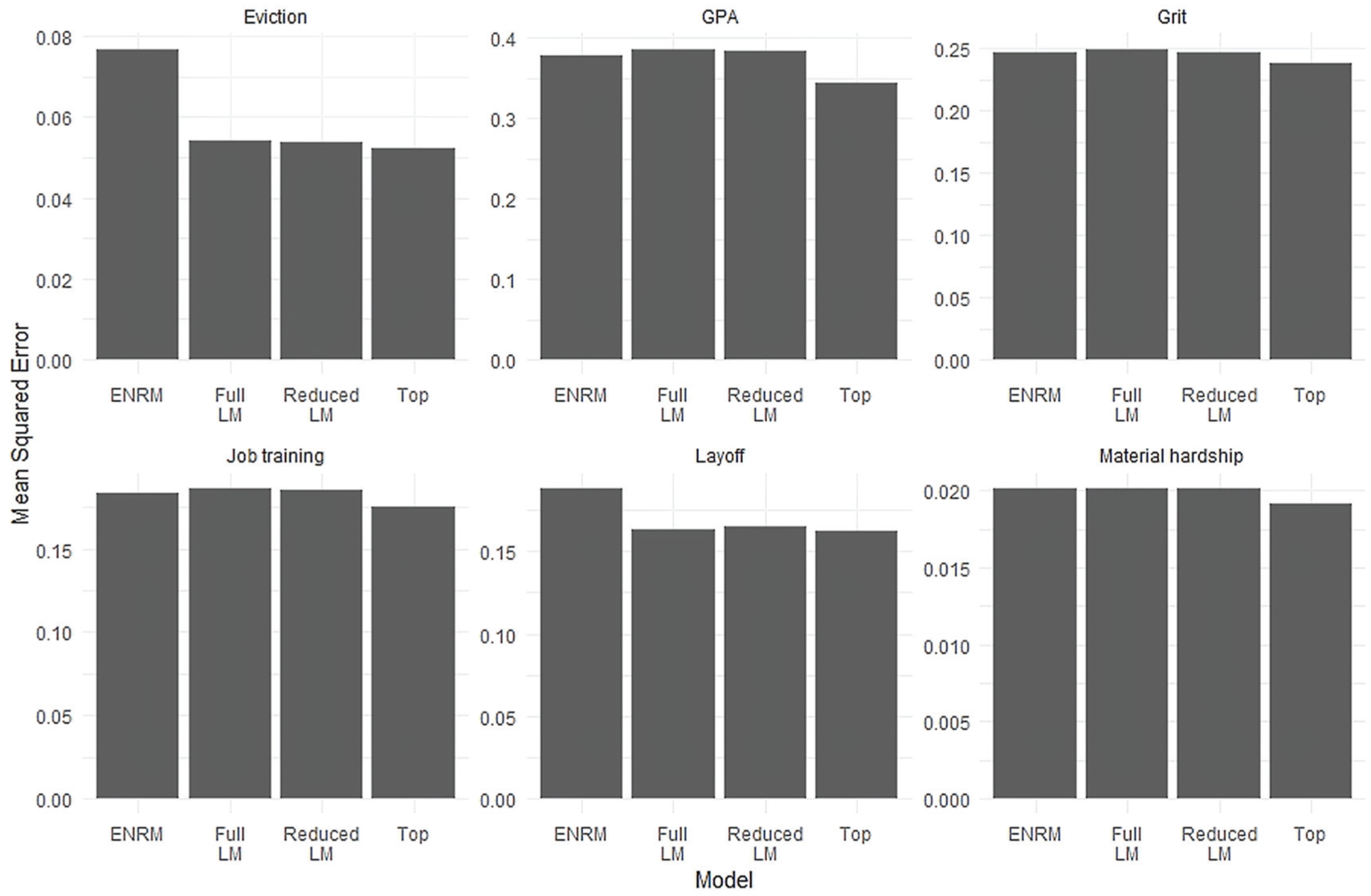
Comparison of prediction scores on holdout data.

Discussion

Cognitive ability and socioeconomic factors are well-documented contributors to individual success and economic security (Mood and Jonsson 2012). This analysis further establishes that these variables are still important in a contemporary sample of at-risk families.

GPA and Grit

GPA and grit were the two outcomes that assessed a focal child’s personal psychological attributes. GPA, although not a direct measure of cognitive ability, is well known to be strongly associated with ability, and provides real-world validity with cognitive ability (Poropat 2009). Grit is a personality trait associated with conscientiousness (Credé, Tynan, and Harms 2016). Both were associated with similar variables, with strong representation by the cognitive test scores, though interestingly, not with teacher assessments of performance from year 5. A variety of socioeconomic variables were associated with both, particularly those related to household income. However, many regression coefficients for the grit models were negative, likely because of ceiling effects, as grit ratings were heavily skewed toward the highest score.

Material Hardship

Material hardship was associated with the largest number of variables selected at both the GBM and ENRM stages. Of these variables, those associated with the ability to pay the rent, mortgage, and other bills were most strongly associated with material hardship. It is unsurprising that these variables tap into later material hardship, particularly because some of these same variables (not paying full amount of rent or mortgage, receiving free food) are derived from the same questions as those used to compose the material hardship scale. Nevertheless, it is worth pointing out that many of these variables are from years 5 and earlier. These variables reliably predicted material hardship more than 10 years later; monitoring changes longitudinally may allow researchers and policy practitioners to identify the most at-risk families, as well as plan future studies and interventions.

Layoffs

Layoffs were associated with similar, but fewer, variables as material hardship. Surprisingly, layoffs were associated with all the variables included that assess failure to pay rent and bills, but only one income variable: household income measured at baseline. Why parents’ layoffs would be associated with their children’s classroom performance and test scores less than income, as well as the parents’ own cognitive ability scores, is an open question.

In modeling layoffs, my ENRMs and GLMs disagreed 10 times as to the sign of a regression coefficient. The GLM is more likely to have estimated the expected sign for most such disagreements, since the ENRM prediction scores were 2 percentage points worse. It is curious that the ENRM had this fault for only this outcome variable.

Eviction

Although eviction followed a pattern similar to what was observed for GPA and grit, the outcome was not associated with as many variables, though of these, the only cognitive variable it was associated with was the focal child’s WJ year 9 passage comprehension test score. The other associations were with a mix of income, bill payment, and risky employment variables.

Job Training

Job training was predicted by a large selection of variables, though not as many as material hardship. Unlike layoffs, job training was associated with many more income and employment measures, but not as many bill payment variables.

Generally, I found broad commonalities in which variables were influential in predicting each of the six life outcomes under study: cognitive ability variables were associated with positive outcomes, and negative socioeconomic variables were associated with negative outcomes. On one hand, it makes sense for a child’s test scores to be linked to GPA, but it is not obvious that these scores should also be linked to the likelihood that a primary caregiver would be laid off or the family would be evicted from their home. This suggests that these variables are interrelated, which also corroborates existing theory (Ermisch, Jäntti, and Smeeding 2012) linking parental behavior, social circumstances, and psychological factors such as cognitive ability and mental health, for example, disorders such as depression and posttraumatic stress (McLoyd and Wilson 1991).

Cognitive ability is highly heritable (Bartels et al. 2002; Briley and Tucker-Drob 2013), and social circumstances are usually also passed on from parents to children through their shared environments: the home, the neighborhood, and the larger community (Attree 2004, Deary et al. 2005). Unfortunately, purely observational studies are not well suited to disentangling these mutually confounded variables, making causal assertions in this context imprudent.

Methodological Issues and Limitations

In a setting such as the FFC, different submissions are likely to identify many of the same major predictors of success, and if new influential factors are to be found, it is likely that their influence will be small, otherwise most models would detect them, and they would already be known in the literature. There are exceptions, such as variables that have not been measured before. Nevertheless, in many cases, including mine, no new standout variables were identified. However, significant value lies in evaluating the approach, both its strengths and weaknesses.

The initial GBM stage of analysis identified 12 variables of importance. However, as my subsequent analyses and documented submissions to the FFC demonstrated, the GBM missed many variables that provided good explanatory and predictive value. Admittedly, some low-variance variables could not be analyzed using GBMs, but this highlights a further limitation of GBMs: although they can handle a very large number of variables as well as missing values, there are still limitations to the data they can work with and the explanatory output they produce.

As mentioned, multiply imputed data sets are not well suited for producing point estimates. Imputation and facilitation software packages often do not allow the user to do this out of the box, and even if one does generate a point estimate, information will be lost in the process. Reconciling prediction difficulties with the uncertainty of imputation techniques or other analytic methods, notably Bayesian analyses, is no small task. It requires rethinking how we evaluate prediction models in order to harness the information conveyed by uncertainty.

My elastic net regression and generalized linear prediction models also highlighted some minor strengths and weaknesses of ENRMs with these variables. The ENRMs’ selection of variables was effective, as the reduced GLMs made better predictions than the full GLMs in most cases. However, the ENRMs themselves were often not as good at making predictions as the GLMs. Traditional modeling approaches may be preferred over ENRMs for making predictions with these types of data, but ultimately, these results (Figure 2) demonstrate that the choice of regression technique one uses to make predictions is not an especially influential decision.

A broader issue with my analysis is that associating variables from various waves in multiple regression models is a cross-sectional, static approach, whereas much of the data are longitudinal in reality (Ganzach 2011). This is a common issue, particularly when machine learning is used. However, to improve on this requires the creation of composite variables, which itself requires a priori knowledge, takes considerable time and effort on the part of the researchers, and most relevantly, is at odds with the hands-off approach used in this analysis, and in high dimensional machine-learning analyses more generally.

On the other hand, my approach had numerous strengths. I was able to conduct all the analyses alone, in a relatively short time frame. The approach is transparent, the analytic steps are clear and easily followed and reproduced in the attached code. The final prediction models were both strong performers and revealed the meaningful variables driving their predictions. By focusing on a few simple, powerful predictors, my models are parsimonious and not overfitted, giving them the potential to make substantive contribution to larger ensemble models.

Conclusions

This analysis of the Fragile Families data showcases how one can use a relatively simple, straightforward approach to modeling to begin selecting and identifying meaningful predictors and build a model with good prediction accuracy. This approach began at a standpoint with few preconceptions, and with these types of sociological data, the approach corroborated known science on the importance of cognitive abilities and economic advantages for six distinct, important outcome variables.

Supplemental Material

SRD-17-0117 – Supplemental material for Leveraging Multiple Machine-Learning Techniques to Predict Major Life Outcomes from a Small Set of Psychological and Socioeconomic Variables: A Combined Bottom-up/Top-down Approach

Supplemental material, SRD-17-0117 for Leveraging Multiple Machine-Learning Techniques to Predict Major Life Outcomes from a Small Set of Psychological and Socioeconomic Variables: A Combined Bottom-up/Top-down Approach by Drew M. Altschul in Socius

Supplemental Material

SRD819943_SM – Supplemental material for Leveraging Multiple Machine-Learning Techniques to Predict Major Life Outcomes from a Small Set of Psychological and Socioeconomic Variables: A Combined Bottom-up/Top-down Approach

Supplemental material, SRD819943_SM for Leveraging Multiple Machine-Learning Techniques to Predict Major Life Outcomes from a Small Set of Psychological and Socioeconomic Variables: A Combined Bottom-up/Top-down Approach by Drew M. Altschul in Socius

Footnotes

Acknowledgements

Funding for the Fragile Families and Child Wellbeing Study was provided by the Eunice Kennedy Shriver National Institute of Child Health and Human Development through grants R01HD36916, R01HD39135, and R01HD40421 and by a consortium of private foundations, including the Robert Wood Johnson Foundation. Funding for the FFC was provided by the Russell Sage Foundation. I would like to thank Ella Edginton for her helpful comments. The results in this article were created with software written in R version 3.4.3 (R Development Core Team, Vienna, Austria) using the following packages: caret 6.0-78 (Williams et al. 2017), taRifx 1.0.6 (Friedman 2013), gbm 2.1.3 (Ridgeway 2007), mice 2.46.0 (Buuren and Groothuis-Oudshoorn 2011), glmnet 2.0-13 (Friedman et al. 2010), matrix 1.2-12 (Bates and Maechler 2017), MuMIn 1.40.4 (Barton 2018), and ggplot2 2.2.1 (Wickham 2016). Replication code for this article is available with the manuscript on the Socius website.

Funding

The author disclosed receipt of the following financial support for the research, authorship, and/or publication of this article: This work was partly undertaken in the University of Edinburgh Centre for Cognitive Ageing and Cognitive Epidemiology, part of the cross-council Lifelong Health and Wellbeing Initiative; funding from the Biotechnology and Biological Sciences Research Council and Medical Research Council is gratefully acknowledged (MR/K026992/1). This work was also supported by a Medical Research Council Mental Health Data Pathfinder award (MC_PC_17209).

ORCID iD

Drew M. Altschul

Supplemental Material

Supplemental material for this article is available with the manuscript on the Socius website.

Author Biography

Drew M. Altschul is a postdoctoral researcher in cognitive epidemiology with Mental Health Data Science Scotland and the Centre for Cognitive Ageing and Cognitive Epidemiology at the University of Edinburgh. He studies the origins of health differences and inequalities from a psychological, socioeconomic, and evolutionary perspective. His current research explores the relationships between early-life social and psychological factors and later life mental illness, using data science techniques with large longitudinal samples.

References

Attree

Pamela

. 2004. “Growing up in Disadvantage: A Systematic Review of the Qualitative Evidence.” Child: Care, Health and Development 30(6):679–89.

Azur

Melissa J.

Stuart

Elizabeth A.

Frangakis

Constantine

Leaf

Philip J.

2011. “Multiple Imputation by Chained Equations: What Is It and How Does It Work?” International Journal of Methods in Psychiatric Research 20(1):40–49.

Bartels

Meike

Marjolein

J. H.

Rietveld

Van Baal

Caroline M.

Boomsma

Dorret I.

2002. “Heritability of Educational Achievement in 12-year-olds and the Overlap with Cognitive Ability.” Twin Research and Human Genetics 5(6):544–53.

Barton

Kamil

. 2018. “Package ‘MuMIn.’” Retrieved February 2, 2018 (https://CRAN.R-project.org/package=MuMIn).

Bates

Douglas

Maechler

Martin

. 2017. “Package ‘Matrix.’” Retrieved February 2, 2018 (https://CRAN.R-project.org/package=Matrix).

Briley

Daniel A.

Tucker-Drob

Elliot M.

2013. “Explaining the Increasing Heritability of Cognitive Ability across Development: A Meta-analysis of Longitudinal Twin and Adoption Studies.” Psychological Science 24(9):1704–13.

Buuren

Stef van

Groothuis-Oudshoorn

Karin

. 2011. “mice: Multivariate imputation by chained equations in R.” Journal of Statistical Software 45(3):1–68.

Credé

Marcus

Tynan

Michael C.

Harms

Peter D.

2016. “Much Ado about Grit: A Meta-analytic Synthesis of the Grit Literature.” Journal of Personal and Social Psychology 113(3):492–511.

Deary

Ian J.

Taylor

Michelle D.

Hart

Carole L.

Wilson

Valerie

Smith

George Davey

Blane

David

Starr

John M.

2005. “Intergenerational Social Mobility and Mid-life Status Attainment: Influences of Childhood Intelligence, Childhood Social Factors, and Education.” Intelligence 33(5):455–72.

10.

Elith

Jane

Leathwick

John R.

Hastie

Trevor

. 2008. “A Working Guide to Boosted Regression Trees.” Journal of Animal Ecology 77(4):802–13.

11.

Ermisch

John

Jäntti

Markus

Smeeding

Timothy

eds. 2012. From Parents to Children: The Intergenerational Transmission of Advantage. New York: Russell Sage.

12.

Friedman

Ari

. 2013. “Package ‘taRifx.’” Retrieved February 2, 2018 (https://CRAN.R-project.org/package=taRifx).

13.

Friedman

Jerome

Hastie

Trevor

Tibshirani

Rob

. 2010. “Regularization Paths for Generalized Linear Models via Coordinate Descent.” Journal of Statistical Software 33(1):1.

14.

Ganzach

Yoav

. 2011. “A Dynamic Analysis of the Effects of Intelligence and Socioeconomic Background on Job-market Success.” Intelligence 39(2):120–29.

15.

Joe

Harry

Zhu

Rong

. 2005. “Generalized Poisson Distribution: The Property of Mixture of Poisson and Comparison with Negative Binomial Distribution.” Biometrical Journal 47(2):219–29.

16.

Mayr

Andreas

Binder

Harald

Gefeller

Olaf

Schmid

Matthias

. 2014. “The Evolution of Boosting Algorithms.” Methods of Information in Medicine 53(6):419–27.

17.

McLoyd

Vonnie C.

Wilson

Leon

. 1991. “The Strain of Living Poor: Parenting, Social Support, and Child Mental Health.” Pp. 105–35 in Children in Poverty: Child Development and Public Policy, edited by Huston

A. C.

New York: Cambridge University Press.

18.

Mood

Carina

Jonsson

Jan O.

2012. “Socioeconomic Persistence across Generations: Cognitive and Non-cognitive Processes.” Pp. 53–84 in From Parents to Children: The Intergenerational Transmission of Advantage, edited by Ermisch

John

Jäntti

Markus

Smeeding

Timothy M.

New York: Russell Sage.

19.

Ogutu

Joseph O.

Piepho

Hans-Peter

Schulz-Streeck

Torben

. 2011. “A Comparison of Random Forests, Boosting and Support Vector Machines for Genomic Selection.” P. S11 in BMC Proceedings, Vol. 5. BioMed Central.

20.

Poropat

Arthur E.

2009. “A Meta-analysis of the Five-factor Model of Personality and Academic Performance.” Psychological Bulletin 135(2):322–38.

21.

Ridgeway

Greg

. 2007. “Generalized Boosted Models: A Guide to the Gbm Package.” Update 1(1):2007.

22.

Salganik

Matthew J.

Lundberg

Ian

Kindel

Alexander T.

McLanahan

Sara

. 2019. “Introduction to the Special Collection on the Fragile Families Challenge.” Socius 5. doi:10.1177/2378023119871580.

23.

Strenze

2007. “Intelligence and Socioeconomic Success: A Meta-analytic Review of Longitudinal Research.” Intelligence 35(5):401–26.

24.

Wickham

Hadley

. 2016. ggplot2: Elegant Graphics for Data Analysis. New York, NY: Springer.

25.

Williams

Chris Keefer

Engelhardt

Allan

Cooper

Tony

Mayer

Zachary

Ziem

Andrew

Scrucca

Luca

Tang

Yuan

Candan

Can

Hunt

Tyler

Kuhn

Max

. 2017. “Package ‘Caret.’” Retrieved December 6, 2018 (https://cran.r-project.org/web/packages/caret/caret.pdf).

26.

Witten

Ian H.

Frank

Eibe

Hall

Mark A.

Pal

Christopher J.

2016. Data Mining: Practical Machine Learning Tools and Techniques. Burlington, MA: Morgan Kaufmann.

27.

Zou

Hui

Hastie

Trevor

. 2005. “Regularization and Variable Selection Via the Elastic Net.” Journal of the Royal Statistical Society: Series B (Statistical Methodology) 67(2):301–20.

Supplementary Material

Please find the following supplemental material available below.

For Open Access articles published under a Creative Commons License, all supplemental material carries the same license as the article it is associated with.

For non-Open Access articles published, all supplemental material carries a non-exclusive license, and permission requests for re-use of supplemental material or any part of supplemental material shall be sent directly to the copyright owner as specified in the copyright notice associated with the article.

0.01 MB

0.00 MB

0.39 MB