Sage Journals: Discover world-class research

Abstract

Computer science has devised leading methods for predicting variables; can social science compete? The author sets out a social scientific approach to the Fragile Families Challenge. Key insights included new variables constructed according to theory (e.g., a measure of shame relating to hardship), lagged values of the target variables, using predicted values of certain outcomes to inform others, and validated scales rather than individual variables. The models were competitive: a four-variable logistic regression model was placed second for predicting layoffs, narrowly beaten by a model using all the available variables (>10,000) and an ensemble of algorithms. Similarly, a relatively small random forest model (25 variables) was ranked seventh in predicting material hardship. However, a similar approach overfitted the prediction of grit. Machine learning approaches proved superior to linear regression for modeling the continuous outcomes. Overall, social scientists can contribute to predictive performance while benefiting from learning more about data science methods.

Keywords

fragile families logistic regression data science random forests

In the Fragile Families Challenge (FFC), participants predicted six socioeconomic outcomes for respondents to the Fragile Families and Child Wellbeing Study (FFCWS) at age 15, on the basis of information on those families between birth and the age of 9.¹ Here I describe my efforts, as a working social scientist with limited knowledge of “machine learning” (ML), to predict the relevant outcomes.²

Data Preparation

The data comprised 12,942 variables relating to 4,242 respondents to the FFCWS. Data were collected in five waves: at the birth of a sampled child and then at ages 1, 3, 5, and 9. A further six variables—the outcomes of interest—were available for half of those families when the relevant child was aged 15. Data were provided in a comma-separated values format, along with documentation relating to the questions and constructed variables. The competition required participants to provide the best predictions for the half of families that did not have age 15 outcomes provided but were known to the organizers, having been set aside randomly. Participants were free to use whatever software and methods they preferred.

The variables available for predictive purposes included data with the full range of measurement levels: interval or ratio variables (e.g., income), ordinal variables (life satisfaction), and categorical variables (whether received food stamps). The six outcomes included three that were dichotomous (eviction, training, and layoffs) and three that were closer to an interval or ratio scale (grade point average [GPA], grit, and material hardship; although see later discussion).

Missing Data

For many variables, responses could be “missing.”³ There are many well-known ways of handling missing data, depending on the reasons why data might be missing (Allison 2001). I decided, after some initial testing,⁴ to treat missing data as valid values when using categorical data, so that, for example, a person’s occupational status might be professional, clerical, other occupations, or missing. For continuous data, such as income, a new binary variable was created to indicate that income data were missing, with the original variable set to 0. Part of my logic was the pattern of attrition: data were often missing through attrition, and families not present in some waves would be less likely to be included at the age 15 wave, in which case the predictions for such cases would not affect the scores.

Creating New Variables

I produced a single R file that created and recoded variables and ran models, with most of the content (700 of 1,000 lines) devoted to creating new variables. Some variables were created to fit into social science knowledge: I created a variable with value 1 when people had reported zero hardship at the previous two waves, to capture the idea that a sense of “shame” might restrict respondents from admitting a deficit in material hardship. It might also capture strong budgeting skills whereby respondents avoided hardship despite low incomes.

I expected that income would be a reliable independent variable in models. Boxplots were used to identify income outliers, and incomes were then top-coded at $100,000 for mothers’ income and $125,000 for fathers’ incomes.⁵

Methods

Overall Approach to Variable Selection and Model Building

The strategy followed had two stages. In the first stage, shortlists of predictor variables were generate using (1) social science knowledge of variables likely to be associated with the outcome (e.g., incomes and material hardship) and (2) simple bivariate correlations between the outcomes and the sets of independent variables. In the second stage, having selected down to manageable numbers of variables, model tests of significance (Akaike information criterion, t tests, R²) were used to further reduce the sets of candidate variables to a final set within the linear models. This latter stage was guided by some of the tools in the rms package (Harrell 2017).

For the dichotomous outcomes, simple binary logistic regression was used.⁶ For the continuous outcomes, initial analysis was conducted using ordinary least squares (OLS), but in the latter part of the competition this was replaced with random forests using the party library (Hothorn et al. 2005; Strobl et al. 2007, 2008). That permitted the inclusion of more variables, with less concern about overfitting, and avoided resolving difficult questions about model specification. Linear models have strong advantages, but it does not take long to see their flaws as predictive models. It is possible, for instance, that marital status may be important for lower income families, and not higher income families, or indeed that higher incomes may matter up to a point, but not beyond that. There are ways to try to capture this within regression (e.g., interaction terms, transformations such as logarithms), but this soon ends up as an ad hoc exercise with clear risks for overfitting.

Social Science Knowledge

As a social scientist I had knowledge of some key domains, particularly material hardship (Mayer and Jencks 1989; McKay 2004) and the risk of layoffs (Bell and Blanchflower 2010). I knew, for example, that models of material hardship were likely to require different measures of income (resources), ability to manage (education), measures of household size and needs (number of children), and experience of hardship. Variables relating to layoffs were also likely to include those capturing human capital (education), position in the labor market (occupation and earnings), and perhaps discrimination (ethnic group). There is also recent work concerning grit (Duckworth 2016), but it is perhaps harder to quickly identify the main causal variables.

There were also two general principles to variable selection that are guided by social science training. First was the persistence of variables over time. In a longitudinal study, current values will often reflect past values. Models may make better predictions by using lagged values of the dependent variable. It was possible to find clear precursors for the constructed variables of grit and material hardship. In practice, this yielded variables that had high degrees of correlation with the wave 6 variables, at least within the training data set. The bivariate correlation between hardship at waves 5 and 6 was 0.394, between grit was 0.14, for evictions was 0.12, and for job training was 0.14. Overall the “persistence” approach was used in models of material hardship and for predicting grit, but not for layoffs. However, although I think this is a sound strategy, the long gap between the latter two waves (six years) will reduce its effectiveness. Moreover, taking past values of variables ran into the problem that wave 6 variables are often based on the primary caregiver, whereas variables at earlier waves are often for the mother. Hence, a past value of layoffs (for the mother) might be a poor predictor of layoffs for the primary caregiver.

The second principle of variable selection was the interdependence of the outcomes. The six outcomes to be modeled turned out to be interrelated, and three pairs of variables stood out as having relatively strong correlations between them:

material hardship and eviction (Pearson’s r = 0.39),

grit and GPA (r = 0.21), and

material hardship and layoff (r = 0.19).

Having good predictions of some of these variables may be useful in models of some of the others, by including the predicted value of (say) hardship in the model for (say) eviction, or the reverse, or a model prediction of grit in the model for GPA. More narrowly, there was also some overlap in the definitions of eviction and material hardship (the latter subsumes the former), and a good model for one should be helpful in finding a better model for the other.⁷

Scales

Survey researchers frequently make use of “scales”—the summation of related questions—to measure unobserved or latent concepts with greater reliability (DeVellis 2016). The FFCWS includes several sets of related questions (Bendheim-Thoman Center for Research on Child Wellbeing 2013). In some cases, their team constructed an overall scale (such as for the Peabody Picture Vocabulary test [Dunn and Dunn 1997] and the Woodcock-Johnson comprehension test [Woodcock, McGrew, and Mather, 2001]). In other instances, there are related questions that I used to create scales using existing practice (externalizing behavior scale from the Strengths and Difficulties Questionnaire; Goodman 1997) and some questions for which a scale seemed appropriate (financial help from friends and family).

I decided to use scales wherever possible in line with a “social science” conceptualization of the problem. Well-validated and reliable series of questions could potentially be more informative than the individual questions that constituted them. So the final model for grit included plus measures based on cognitive ability: the model of material hardship included scales of material hardship from the previous waves, plus a scale for the kinds of financial help available to families.⁸

Models and Results

Models

The statistical approaches generally used for continuous variables are linear regression and binary logistic regressions for dichotomous outcomes. In statistical terms, the first three outcomes are not strictly continuous variables, as their values constitute only a relatively small number of fixed points—13 for GPA, 12 for grit, and 10 for material hardship⁹—I switched from linear regression to random forest models for the first three outcomes (GPA, grit, and material hardship) with random forests leading to small gains in predictive performance.¹⁰

Material Hardship

I developed models for material hardship using conditional inference trees (“random forests”).¹¹ I used only a small number of variables (25), which were generally past values of material hardship, plus measures of incomes, needs, and human capital.

Random forests do not provide easy means of identifying the predictor variables with the greatest effect on the outcome, but measures of “variable importance” have been developed. These compare the model’s predictive accuracy by replacing each variable, in turn, with a randomized version of that variable; predictive accuracy falls if that variable is important and barely changes if it is unimportant.

Figure 1 shows the importance of different variables. The variable with the highest importance score was material hardship measured at wave 5. Other variables with high importance scores included wave 4 material hardship, having never been in material hardship at waves 4 and 5, and wave 4 and 5 measures of phone disconnection. These latter variables may signal a “last resort” reaction to adversity. Other variables with sizable importance scores included measures of income and the ability of family or friends to provide assistance.

Figure 1.

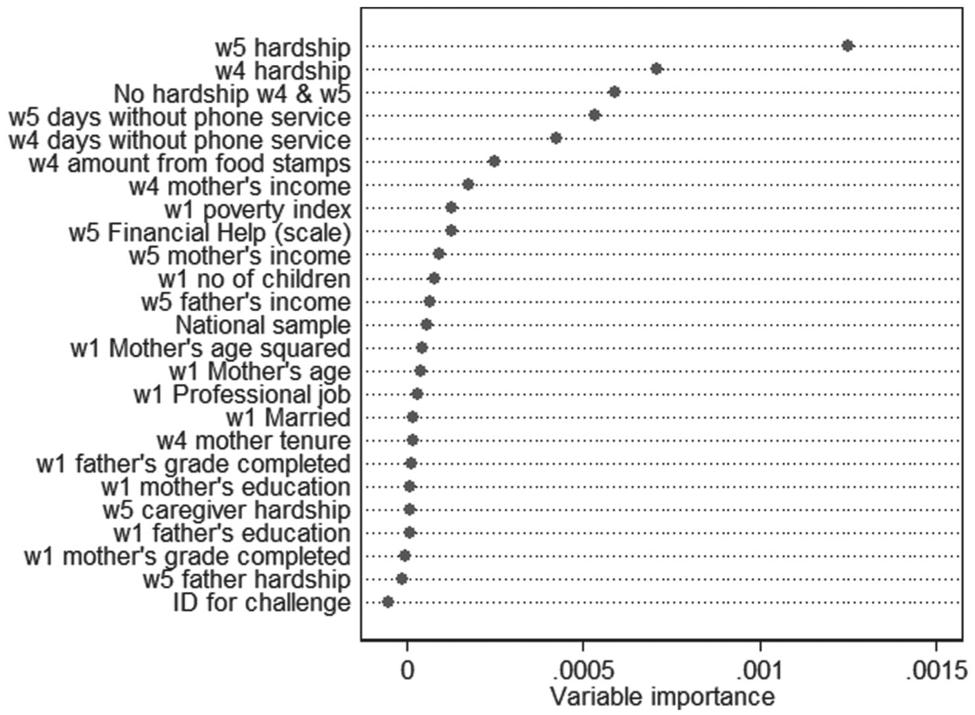
Variable importance measures for material hardship model (final stage, seventh ranked on holdout data).

Grit

The model for grit followed the same approach as for material hardship but included only 10 variables. The variables, and their importance, are shown in Figure 2. Grit measured at wave 5 did not seem to be particularly important, nor other questions used in the grit scale, and neither was the constructed scale of Strengths and Difficulties Questionnaire externalizing behavior. The two key factors seemed to be measures of cognitive ability. Also of some importance to the predictive performance were the gender of the child and whether a caregiver had called the child “dumb or lazy or some other name like that” at the preceding wave.

Figure 2.

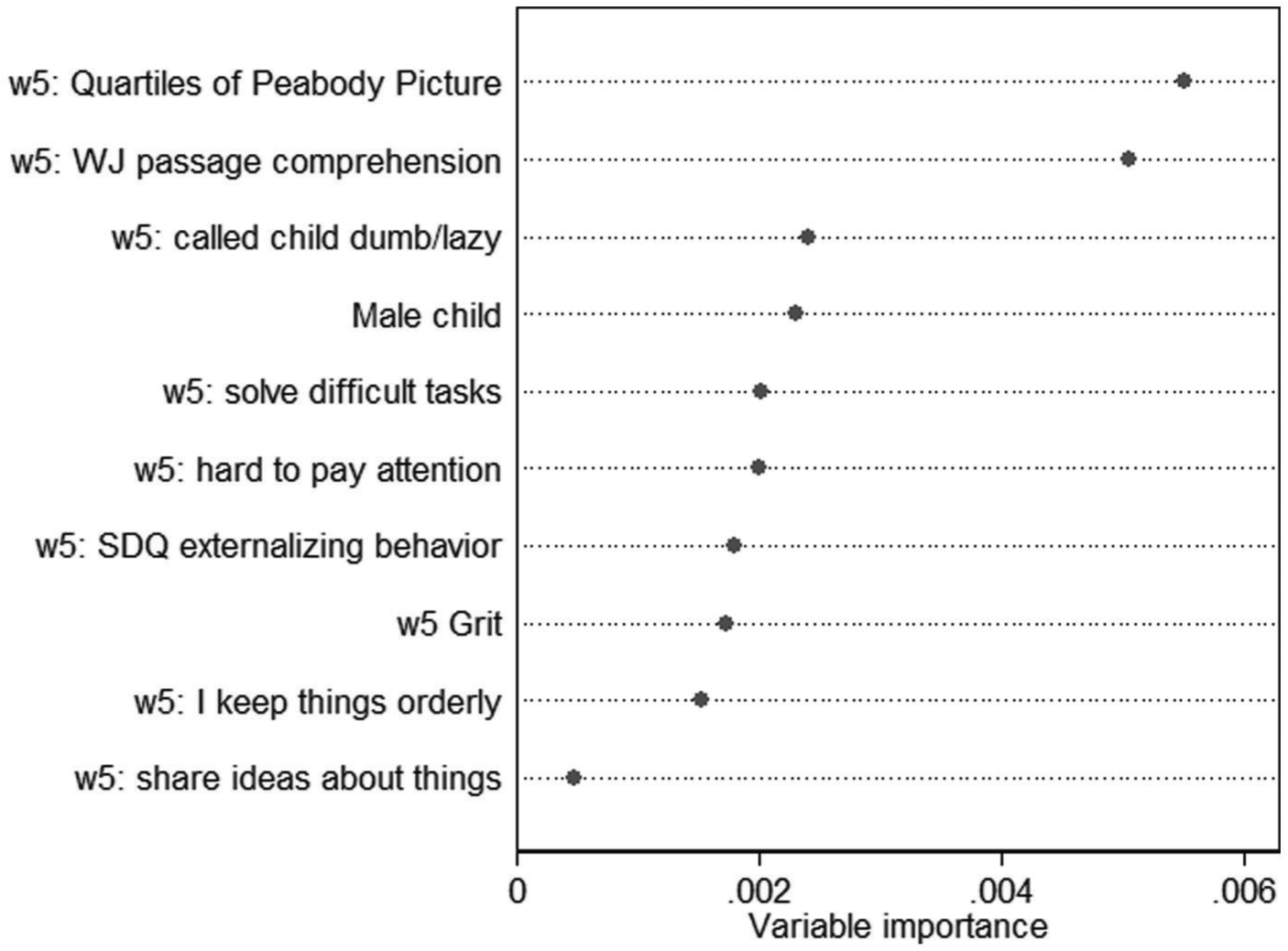
Variable importance measures for grit model (final stage, 17th ranked on holdout data, 1st on public leaderboard).

Although the model for grit attained the lead ranking on the public leaderboard, it ranked 17th in the final held-out data. This suggests a degree of overfitting. In practice, I worked a great deal on this outcome and submitted dozens of different models. As such, the models were likely to have evolved to fit the nuances of the leaderboard data and did less well on the held-out data (Blum and Hardt 2015).¹²

Job Layoffs

The model for job layoff was a standard logistic regression including just four variables¹³ (Table 1). The most principled variable included was predicted material hardship, which was strongly associated with the likelihood of job layoff. The level of mother’s income, and whether father’s reported income was zero, were also included in the model and were statistically significant at standard levels. A single dummy variable from the set of occupational codes, being at an “executive level,” was also included was positively associated with the risk for being laid off from a job compared to other occupations.

Table 1.

Logistic Regression Model of Layoff (Final Model, Second on Holdout Data).

Variable	Coefficient (SE)
Predicted value of material hardship	4.110*** (1.516)
Father’s income is zero at wave 5	0.709** (0.329)
Mother’s wave 5 income	−0.00001** (0.00000)
Executive occupation	0.541** (0.244)
Constant term	−1.570*** (0.240)
Observations = 1,277
Log likelihood = −636.987
Akaike information criterion = 1,283.974

p < .05. ***p < .01.

Earlier models had included levels of education and the “race” of the mother. These were part of a model that was leading at the midway point of the FFC (on the held-out data) but were not retained (and did not appear significant) once the prediction of material hardship was included. This model is included in the online supplement.

Other Models: GPA, Eviction, and Job Training

Full details of the results from the submitted models are shown in Table 2, and model results in the online appendix. Less time was spent on the other three outcomes, but a few observations may interest analysts. In the model of GPA, predicted material hardship had among the highest variable importance, but predicted grit did not. The logistic regression model for eviction included significant effects from wave 5 material hardship, mother’s education, and the amount of rent being paid. The logistic regression model for job training, which placed 19th on the final data, included statistically significant effects from wave 5 income, ethnic group, past training experience, and wave 5 hardship.

Table 2.

Scores from Progress Stage and Final Stage of Fragile Families Challenge.

Stage	GPA	Grit	Material Hardship	Eviction	Layoff	Job Training
Holdout data
Baseline (mean prediction)	0.4251	0.2530	0.0249	0.0555	0.1672	0.1853
Progress stage	0.3588	0.2440	0.0197	0.0557	0.1657	0.1801
Final stage	0.3628	0.2425	0.0197	0.0570	0.1626	0.1806
Ranks (1–161)	31	17	7	108	2	19
Public leaderboard
Baseline (mean prediction)	0.39273	0.21997	0.02880	0.05341	0.17435	0.20224
Progress stage	0.37208	0.20720	0.02435	0.04610	0.16778	0.19788
Final stage	0.37044	0.20701	0.02468	0.04947	0.16653	0.20666
Notes		First on public board			Progress prize^a

That is, the leading score on the hold-out data of the models submitted by a deadline at the mid-point of the Fragile Families Challenge.

Discussion and Conclusions

The papers at the scientific workshop following the FFC (https://www.youtube.com/playlist?list=PLbavk6eDjgUSghfps3elbgD-uV8VAK4QH) suggest that most participants were using “ML” approaches with rather less emphasis on social science understanding. Here I argue that an approach based largely on social science understanding can be competitive with even the best of such approaches, using surprisingly small subsets of the data.

The principal social scientific ideas applied here were as follows. I used my knowledge of the six outcomes as the main approach to selecting variables, such as a past denial of hardship as a predictor of hardship. I also selected variables that were similar to the targets if they appeared in earlier waves (e.g., on grit). I used scales where possible.

I also note that all the final prizes were won by teams (one of three members, the others rather larger), which may imply that there are strengths to a team collaboration, perhaps in terms of ideas or the ability to delegate tasks on which people could specialize (such as data preparation or imputation). Teams mixing data science and social science might achieve even more.

Lessons for Social Science Training

The United Kingdom has a long history of concerns about the quantitative skills of its social scientists (British Academy 2012), particularly compared with the United States. Partly this relates to a lack of appropriate training during the doctoral period. Key priorities for social science training might include

knowledge of replication and open science more generally (Freese 2007; Stodden, Seiler, and Ma, 2018) and

understanding of ML, which seems to have proceeded in computer science to the relative ignorance of social statistics.

Both would have enhanced my ability to contribute to the FFC.

Supplemental Material

annex_other_results – Supplemental material for When 4 ≈ 10,000: The Power of Social Science Knowledge in Predictive Performance

Supplemental material, annex_other_results for When 4 ≈ 10,000: The Power of Social Science Knowledge in Predictive Performance by Stephen McKay in Socius

Footnotes

Acknowledgements

I am grateful to the four anonymous reviewers and the editors for their cogent comments on this article, which led to significant improvements. I am also grateful to participants in the closing scientific workshop of the FFC for their helpful and generous feedback.

Author’s Note

The results in this report were created with software written in R 3.4.1 (R Core Team 2017) using the following packages: tidyverse 1.2.1 (Wickham 2017), party (Hothorn et al. 2005; Strobl et al. 2007, 2008), rms 5.1-1 (Harrell 2017), and stargazer 5.2 (Hlavac 2015). Replication code for this article is available at .

Funding

The author(s) disclosed receipt of the following financial support for the research, authorship, and/or publication of this article: Funding for the FFCWS was provided by the Eunice Kennedy Shriver National Institute of Child Health and Human Development through grants R01HD36916, R01HD39135, and R01HD40421 and by a consortium of private foundations, including the Robert Wood Johnson Foundation. Funding for the FFC was provided by the Russell Sage Foundation. This research received no specific grant from any funding agency in the public, commercial, or not-for-profit sectors.

ORCID iD

Stephen McKay

Supplemental Material

Supplemental material for this article is available with the manuscript on the Socius website.

Notes

Author Biography

Stephen McKay is distinguished professor in social research at the University of Lincoln (UK). His research uses quantitative tools to analyze inequalities of income and wealth, including in his book Wealth and the Wealthy (with K. Rowlingson). He is currently looking at ways to address panel attrition in social surveys.

References

Allison

Paul D.

2001. “Missing Data.” Sage University Papers Series on Quantitative Applications in the Social Sciences 07-136. Thousand Oaks, CA: Sage.

Bell

David N.

Blanchflower

David G.

2010. “UK Unemployment in the Great Recession.” National Institute Economic Review 214(1):R3–25.

Bendheim-Thoman Center for Research on Child Wellbeing. 2013. “Scales Documentation and Question Sources for the Nine-year Wave of the Fragile Families and Child Wellbeing Study.” Princeton, NJ: Princeton University.

Blum

Avrim

Hardt

Moritz

. 2015. “The Ladder: A Reliable Leaderboard for Machine Learning Competitions.” arXiv. Retrieved October 27, 2018 (https://arxiv.org/abs/1502.04585).

British Academy. 2012. “Society Counts: Quantitative Skills in the Social Sciences and Humanities.” London: British Academy. Retrieved ( https://www.britac.ac.uk/sites/default/files/BA%20Position%20Statement%20-%20Society%20Counts.pdf).

DeVellis

Robert F.

2016. Scale Development: Theory and Applications. 4th ed. London: Sage Ltd.

Duckworth

Angela

. 2016. Grit: The Power of Passion and Perseverance. New York: Simon & Schuster.

Dunn

Loyd M.

Dunn

Leota M.

1997. “Peabody Picture Vocabulary Test.” 3rd ed. Circle Pines, MN: American Guidance Service.

Fielding

Alan H.

Bell

John F.

1997. “A Review of Methods for the Assessment of Prediction Errors in Conservation Presence/Absence Models.” Environmental Conservation 24(1):38–49.

10.

Firth

David

. 1993. “Bias Reduction of Maximum Likelihood Estimates.” Biometrika 80(1):27–38

11.

Freese

Jeremy

. 2007. “Replication Standards for Quantitative Social Science: Why Not Sociology?” Sociological Methods & Research 36(2):153–72.

12.

Goodman

Robert

. 1997. “The Strengths and Difficulties Questionnaire: A Research Note.” Journal of Child Psychology and Psychiatry 38(5):581–86.

13.

Grömping

Ulrike

. (2009). “Variable Importance Assessment in Regression: Linear Regression versus Random Forest.” American Statistician 63(4):308–19.

14.

Harrell

Frank

Jr.

2017. “rms: Regression Modeling Strategies.” R Package Version 5.1-1. Retrieved (https://CRAN.R-project.org/package=rms).

15.

Hastie

Trevor

Tibshirani

Robert

Friedman

2017. The Elements of Statistical Learning: Data Mining, Inference, and Prediction. 2nd ed. New York: Springer.

16.

Hlavac

Marek

. 2015. “stargazer: Well-formatted Regression and Summary Statistics Tables.” R Package Version 5.2. Retrieved (https://CRAN.R-project.org/package=stargazer).

17.

Hothorn Buehlmann Dudoit

Sandrine

Molinaro

Annette

Van Der Laan

Mark

. 2005. “Survival Ensembles.” Biostatistics 7(3):355–73.

18.

Gary

King

Zeng

Langche

. 2001. “Logistic Regression in Rare Events Data.” Political Analysis 9(2):137–63.

19.

Mayer

Susan E.

Jencks

Christopher

. 1989. “Poverty and the Distribution of Material Hardship.” Journal of Human Resources 24(1):88–114.

20.

McKay

Stephen

. 2004. “Poverty or Preference? What Do ‘Consensual Deprivation Indicators’ Really Measure?” Fiscal Studies 25(2):201–24.

21.

R Core Team. 2017. “R: A Language and Environment for Statistical Computing.” Vienna, Austria: R Foundation for Statistical Computing.

22.

Salganik

Matthew J.

Lundberg

Ian

Kindel

Alexander T.

McLanahan

Sara

. 2019. “Introduction to the Special Collection on the Fragile Families Challenge.” Socius 5. doi:10.1177/2378023119871580.

23.

Strobl

Carolin

Boulesteix

Anne-Laure

Kneib

Thomas

Augustin

Thomas

Zeileis

Achim

. 2008. “Conditional Variable Importance for Random Forests.” BMC Bioinformatics 9(307). Retrieved (http://www.biomedcentral.com/1471-2105/9/307).

24.

Strobl

Carolin

Boulesteix

Anne-Laure

Zeileis

Achim

Hothorn

Torsten

. 2007. “Bias in Random Forest Variable Importance Measures: Illustrations, Sources and a Solution.” BMC Bioinformatics 8(25). Retrieved (http://www.biomedcentral.com/1471-2105/8/25).

25.

Victoria

Stodden

Seiler

Jennifer

Zhaokun

. 2018. “An Empirical Analysis of Journal Policy Effectiveness for Computational Reproducibility.” Proceedings of the National Academy of Sciences 115(11):2584–89.

26.

van Buuren

Stef, and Karin

Groothuis-Oudshoorn . 2011. “mice: Multivariate Imputation by Chained Equations.” R Journal of Statistical Software 45(3):1–67.

27.

Wickham

Hadley

. 2017. “tidyverse: Easily Install and Load the ‘Tidyverse.’” R Package Version 1.2.1. Retrieved (https://CRAN.R-project.org/package=tidyverse).

28.

Woodcock

Richard W.

McGrew

Kevin S.

Mather

Nancy

. 2001. “Woodcock-Johnson III Tests of Achievement.” Itasca, IL: Riverside.

Supplementary Material

Please find the following supplemental material available below.

For Open Access articles published under a Creative Commons License, all supplemental material carries the same license as the article it is associated with.

For non-Open Access articles published, all supplemental material carries a non-exclusive license, and permission requests for re-use of supplemental material or any part of supplemental material shall be sent directly to the copyright owner as specified in the copyright notice associated with the article.

0.00 MB

0.71 MB