Sage Journals: Discover world-class research

Abstract

The authors present some relatively simple measures for the degree of organization of a social field, illustrating them with the intuitively accessible cases of fields that are organized by geographic space, and demonstrate that the measures are able to indicate when fields become more organized and that they can be applied to nongeographic data. Finally, the general approach highlights the danger of ignoring complexities of the functional form of spatial interdependence for social data.

Keywords

field theory geographic alignment social space

Although field theory has become increasingly popular in sociology (e.g., Armstrong 2002; Barman 2007; Berman 2006; Evans and Kay 2008; Ferguson 1998; Fligstein and McAdam 2012; Go 2008; Haveman, Rao and Paruchuri 2007; Lounsbury, Ventresca, and Hirsch 2003; Quinn 2008; Rawlings and Bourgeois 2005; Ray 1999), sociologists continue to struggle with the problem of how to quantify fields and field effects. To be sure, there are quantitative techniques related to the field theoretic project. In large part because of the influence of work such as Distinction (Bourdieu [1979] 1984), there has traditionally been a close association between correspondence analysis (CA) and Bourdieuean variants of field theory in particular (see Bourdieu and Wacquant 1992:96). Insofar as it taps into the notion of field as topology (see Martin 2003:28), the appeal of CA is clear. Even more, it embraces description (see Benzécri 1991) and the notion of duality (Breiger 2000) that have connections to the field theoretic rejection of mainstream social ontology.

At the same time, the mathematical properties of CA are fundamentally at odds with the insights that led to field theory in the first place. In particular, its physical interpretation is one in which we have masses somehow “held” apart from one another. This vision is somewhat like the “crystalline spheres” of pre-Galilean astronomy, as criticized by the pivotal field theorist Wolfgang Köhler (1947:131). In contrast, the field theoretic approach ala Faraday (also cf. Köhler 1920; Maxwell [1891] 1954) posits dynamic equilibria arising from sets of local nonindependencies that aggregate up into a wholistic field effect.

In this article, we turn to the core principles of field theory in the social sciences, and to the mathematics of random field theory, to derive some extremely simple approaches to measuring the strength and organization of fields in some very particular cases. Although this must be understood as the merest beginnings, we find that these techniques not only are rigorously derivable from the field theoretic perspective but that they shed new light on processes long of interest to social scientists.

An Approach to Measuring Fields

Overall Logic

In the classical field theoretic tradition, a field must be distinguished from space. Whereas space is the necessary backdrop for all our observations, a field exists only where there is evidence of a field effect. The mere fact that social objects or practices can be arranged in some sort of space does not imply the presence of a field effect; correlatively, we can measure a field effect only if we know “where” objects are in space. Hence, we need methods of determining whether there even is a field effect, methods that would have the following two characteristics: first, they would be separable from methods of positioning objects in a space; second, they would be descriptive and independent of the correctness of any particular model, in the way that the mean, standard deviation, and correlation are model-independent descriptions of univariate and bivariate distributions.

Here, we begin with the work of two of the most important of the first generation of field theorists, Kurt Koffka and Wolfgang Köhler. They struggled with two questions: how to conceptualize the processes that generate a field and where to put the field. Regarding the latter, Koffka (1935) argued that although we could perhaps understand field theory as applying to a purely phenomenological matter of the pushes and pulls on each behaving organism (as in Kurt Lewin’s [1951] approach), this approach tends to degenerate into solipsism. We must therefore also pay attention to what he called the “geographic environment,” and only on this basis can we derive the “environmental field.” For we do not find ourselves (as actors) within our own heads (as Lewin’s drawings actually implied) but rather in the world. Thus it is only attention to what is on the other side of our eyeballs that can, or so Koffka argued, stabilize a field theoretic approach.

And indeed, this allows us to follow the most daring of the field theorists, Wolfgang Köhler, in his formulation of the processes that generate fields. Köhler argued that fields were one manifestation of a larger class of self-organizing Gestalts that could be found not only in animal and human life but in physical systems as well. An example he treated at length (Köhler 1920) is the spontaneous distribution of charge along a conductor. The whole snaps into a particular configuration as a result of the compounded local relations of repulsion between nearby electrons. Taking this vision seriously, and wedding it to Koffka’s emphasis on the external environment, allows us to begin the process of turning field theory from a set of loose metaphors to a generative program of research.

To facilitate the development of measures of field effect that are separable from spatial position, we begin with the special case of data that come from units with a geographic basis and thus rely on geographic space to anchor our measures. For purposes of clarity, we link our approach to existing work on spatially located data (although we discuss some of the complexities of such data after the main exposition of the field measures). Only after we have laid out the approach for geographic spaces do we demonstrate the application to a nongeographic “social space.”

The Sociology of Space

It is because social relations are so frequently and inevitably correlated with spatial relations; because physical distances so frequently are, or seem to be, the indexes of social distances, that statistics have any significance whatever for sociology. (Park 1926:14)

Despite our talk of “social space,” geographic space itself is, as Park reminded us, social; indeed, there has been a resurgence of interest in the social dynamics of space in recent years, as well as interest in the use of spatial statistics. In part, this is because of a growing awareness of the various methodological challenges that come with the use of spatially situated data. Careful attention has been paid to two classes of problems in particular: spatial dependence and spatial heterogeneity. Commonly discussed in terms of the idea of spatial autocorrelation, spatial dependence is typically explained in terms of two underlying processes: first, commonalities in measurement or specification error, and second, contamination, whereby the value of an outcome in any locale is affected by the value of the outcome and/or predictors in neighboring locales (Anselin 1988).

Whereas spatial dependence refers to the possibility of a spatially organized error structure, spatial heterogeneity refers to the idea that the parameters of a given model may vary predictably from one place to the next. These instabilities can be conceptualized in terms of both differences across discretely defined regions, as well as in terms of variation across a continuous trend surface. In the discussion below, we bring notions of both dependence and heterogeneity to bear on the problem of trying to measure field effects. More specifically, we go on to suggest that field effects can be quantified by measuring the extent to which heterogeneous coefficients are spatially dependent.

This is, of course, more than just a technical exercise. The importance of the substantive relationship between physical space and social organization has long been a central theoretical point in a number of sociological traditions. This is exemplified not only by the work of old “Chicago school” (e.g., Park, Burgess and McKenzie [1925] 1967) and its descendants (e.g., Morenoff 2003) but by the “new Irvine school” as well (e.g., Butts forthcoming; Hipp, Faris, and Boessen 2012). The common intuition behind these varying schools of thought is that social life is fundamentally situated, thus giving rise to aggregated patterns of interpersonal organization. This suggests various sorts of heterogeneity that are spatially organized. In certain cases, we argue, this spatial organization can be understood as resulting from field processes and hence should be measurable as such.

In laying out our approach, we use the geospatial location of units as a substrate to aid in the conceptualization of the degree of a field effect. Drawing on the accumulated researches of geographers and spatial statisticians, we may expect that even in the absence of a field, we would expect some local spatial autocorrelation, with proximate observations exhibiting at least some degree of statistical dependence. We then go on to make the assumption that, in general, a field effect would lead to orderliness at a translocal scale. When we wonder whether there is “a” political field, we are asking ourselves whether the field effect is strong enough so that politics works the same way in Des Moines, Iowa, as it does in Santa Rosa, California. We later discuss how the techniques we put forward can be adapted to cases in which we imagine a more complex ordering. We thus begin with the notion that the field effect can be measured as the range of autocorrelation across spatially distributed units; after developing our logic for the measure of range, we discuss some related rescalings that may have more intuitively appealing interpretations.

Fields as Correlation Structures

It may help to illustrate the logic; here we draw on the analogy to a magnetic field. This analogy has been widely used by field theorists, as well as being the subject of critique, and a number of theorists have done both (e.g., Bourdieu [1966] 1969:89; [1984] 1988:149). Consider a piece of nonmagnetized iron. The metal may be understood as having a large number of magnetic domains: small areas each having a polarization, but randomly oriented, as in Figure 1a. When placed in a magnetic field, the vectors of polarizations align (see Figure 1b). The larger the field effect, the greater the alignment. This is the motivation for the current approach. What is so useful about this metaphor is that it highlights that a field is an ensemble of vectors—combinations of a direction and a magnitude—that may be felt senses of impulsion, or may be action-dispositions, that are organized by positions. Here we treat each of the vectors as having the potential to be more or less aligned with others.

Figure 1.

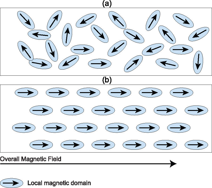
Magnetic field and alignment. (a) No alignment, no overall field. (b) Alignment of local domains produces magnetic field.

The question is how to quantify the degree of alignment. One possibility is to attempt to model the dynamics that may underlie any observed state. This requires having a defensible theory of the nature of the units and their interactive forces. Such models have been developed in animals science since Breder (1954; see Breder 1951 for an earlier attempt) suggested that the aggregate behavior of fish schools arose from simple processes that could be modeled according to physical laws of attraction and repulsion (more recently, see Cavagna et al. 2013; Ginelli et al. 2015; Parrish and Turchin 1997:136). However, even in the absence of such models of dynamics, it is possible to quantify the degree of organization (or “polarization,” as it is called in studies of fish schools).

The exploration of such forms of regularity requires that we have model-independent quantifications of the degree of organization of our data. It is difficult to choose models of processes that would explain our data when we are not yet sure what aspects of the data we are trying to explain. Yet such model-independent measures are not yet on hand for field theoretic analyses. In an effort to bridge this gap, we draw on random field theory, focusing in particular on approaches to quantifying the “range” of order. In the least ordered case, in which every domain is independently oriented, we may say that the order is completely local. In the most ordered case, in which every domain is oriented identically, the order is completely global. In between, we may expect that weaker fields have a lesser range of order.¹

The degree of order at any distance can be understood as the average degree of nonindependence or alignment between measurements at that distance. For reasons to be explicated below, we denote the degree of alignment at any distance R as Γ(R). Although this is known in physics as a correlation function, given the fact that this term is so strongly identified with the Pearson correlation in sociology, we here generally refer to it as “alignment”—some quantification of the degree of similarity between the vectors at two positions. Commensurate with Tobler’s (1970:236) first law of geography (i.e., that “everything is related to everything else, but near things are more related than distant things”), we expect pairs of proximate observations to be more closely aligned than their more distant counterparts. That is, we expect the relationship between distance and alignment to take a form such as that of Figure 2. We see here the degree of alignment beginning to drop off as distance increases, with the rate of change eventually leveling out at a distance of roughly 75 units. In this case, it reaches a floor substantially above zero, because most noncentered distributions of observations will have an expectation of a positive association—they will be more similar than not—between randomly picked realizations.

Figure 2.

Expected relation between distance and alignment.

The graph in Figure 2 is analogous to a correlogram, a commonly used tool in geostatistics in which the notion of range refers to the distance at which pairs of observations begin to exhibit independence.² From this perspective, range refers to the point at which the field effect goes to zero (see, e.g., Chaix et al. 2005). Although our conceptual understanding of the relationship between distance and dependence is consonant with that of geostatistics, a discipline that itself builds heavily on random field theory, our formal approach is more directly inspired by the application of random field theory in materials science.³

We can consider the area under the curve representing the relationship between the alignment of domains and the distance between them, such as the one shown in Figure 2, as the total field mass. We propose that the range of a field effect can be measured by standardizing this mass to highlight its spatial or positional characteristics.⁴ We then go on to consider alternative forms of standardization that attempt to neutralize the effects of space, and thus better express (1) the overall degree of organization of the field as well as (2) the strength of the underlying vectors. The use of standardized measures helps facilitate comparison, with alternative forms of standardization serving to capture previously unacknowledged dimensions of difference. So although there is a natural tendency to assume that in a geographic setting a strong field is a global one, our approach allows the possibility of uncovering strong but relatively local fields.

Quantifying Field Effects

The Autocorrelation Function and Field Effect

As noted above, we begin by turning to results from materials science. Imagine that we have a three-dimensional volume of some sort, with a varying value at any point that can be treated as a vector, and consider the following measure:

L^{2} = \frac{\int R^{2} Γ (R) d^{3} R}{\int Γ (R) d^{3} R},

where R indicates a spatial distance between two points and Γ an alignment function (i.e., the similarity in values across points separated by distance R), and d³R indicates that we are integrating over a three-dimensional volume. Note that Γ is unspecified; all we now require is that it take on extreme values of −1 when the two vectors are opposite and 1 when they are perfectly aligned (−1 ≤ Γ ≤ 1). This is a measure of the range of order in some material (see Ziman 1979:26; also see Köhler 1920:105, 114, 116 for a discussion of related integrals as a measure of field or Gestalt).⁵ Note that the denominator is the alignment function at any distance summed up over all distances in a three-dimensional space. This may be understood as the total amount of similarity in the data. The numerator is nearly identical but weights this by a function of the distance between points (a simple quadratic for the case of three-dimensional space). The further two similar points are, the more the numerator increases. Dividing this numerator by the total similarity, then, tells us how much of the ordering is “far” as opposed to distant. (A somewhat related approach has been used to quantify the spatial organization in similarity in bird songs by Laiolo 2008.) Now consider an analogue for a discrete, two-dimensional case; we accordingly propose

L = \frac{\int R Γ (R) d^{2} R}{\int Γ (R) d^{2} R} = \frac{\sum_{i, j \neq i} d_{i j} g_{i j}}{\sum_{i, j \neq i} g_{i j}},

where g_ij is the alignment and d_ij the distance between areas i and j, as a potential measure of the range of the field effect.

The alert reader will note that the numerator has a form similar to a class of statistics used to quantify the relation between two correlation matrices, often assimilated to the Mantel (1967) test, in which the product of two correlations is investigated. Such a Mantel test entered sociology via network analysis, as one version for the examination of the distribution of such statistics through the quadratic assignment procedure (Baker and Hubert 1981; Hubert 1985; Hubert and Schultz 1976) found a use in the determination of the statistical significance of associations in network data, usually in the form of a permutation test (Krackhardt 1987, 1988, 1992). The most obvious Mantel-type statistic that is relevant for spatial autocorrelation is what is known as Moran’s (1950) I statistic, which is used to describe the nonindependence of a set of cases that are connected to differing degrees (called the “weight” of one case on another) and correlated to different degrees. This statistic may be written

I = \frac{1}{γ} \sum_{i, j} g_{i j} w_{i j} = \frac{1}{γ} \sum_{i, j} r_{i j} w_{i j} = \frac{1}{γ} \sum_{i, j} z_{i} z_{j} w_{i j},

where z is the observation of interest at the ith position, w_ij is the weight linking the ith and jth observations, with the matrix W ={w_ij} row standardized (Σ_iw_ij = 1), the z values mean standardized, and γ = Σ_iz_i² (Anselin 1995). In other words, we assume that the value in any area is in part a function of the values in other areas and that the extent of this interdependence is contained in a weights matrix; because of the mean centering, the alignment function g_ij is identical to the dot-product correlation r_ij between the two observations.

It will be noted, however, that in the classic Mantel test, and in the Moran test, we multiply two similarity matrices; our test statistic grows when pairs are similar in both respects. In many cases, we assume that the weight between the two cases is an inverse function of distance, for example,

I \approx \sum_{i, j} \frac{g_{i j}}{d_{i j}},

which differs from the numerator of equation 2 in that this measure decreases with the distance whereas equation 2 increases. We shall demonstrate that the formulation adopted in equation 2 makes substantive sense for the analyses proposed. Thus, although L is not a conventional Mantel test, many procedures used to determine statistical significance of this class of statistics would be adaptable, although there are limitations of interpretability.⁶ Fortunately, we do not believe such tests necessary for descriptive purposes.

Measures of Field Organization and Strength

The L statistic, then, fulfills our requirements of a measure of the “range” as introduced impressionistically above; the numerator of this expression corresponds to the “total field mass” (the integral of the curve in Figure 2). However, the total mass is difficult to compare across cases, and so it may be useful to consider

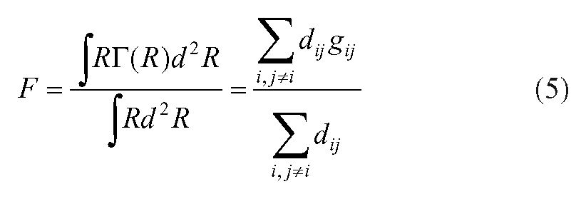
F = \frac{\int R Γ (R) d^{2} R}{\int R d^{2} R} = \frac{\sum_{i, j \neq i} d_{i j} g_{i j}}{\sum_{i, j \neq i} d_{i j}}

as a measure of the overall degree of organization of the field. In other words, we again sum up the distance-weighted alignments across all pairs of areas. But now we normalize this quantity by dividing by the sum of all distances. This aids in comparison of data sets that have different arrangements of positions (such that, say, there is a greater average distance in one than in the other).⁷ Note that if g_ij = 1 for all i and j, F = 1, and if g_ij = 0 for all i and j, F = 0. More important, if there is no overall organization such that we are as likely to observe values of g that are less than 0 as we are to observe values that are greater than 0 (recall that −1 ≤ g ≤ 1), and that there is no spatial pattern to the correlations, we expect F to be 0.

This measure of organization of the field effect, however, is indifferent to the strength of the field effect at any place. Imagine that at every position, our vector is exactly zero. The alignment between any two positions is 1.0, and so by equation 5, the field effect is at its maximum. This is as it should be, for the measure is one of homogeneous organization. But we are also interested in the strength (S) of the field effect and propose

S = F \bar{V} = (\frac{\sum_{i, j \neq i} d_{i j} g_{i j}}{\sum_{i, j \neq i} d_{i j}}) (\frac{1}{N} \sum_{i = 1}^{N} | v_{i} |),

where v_i is the vector at position i. Thus we are weighting the field effect by the average vector magnitude.⁸

We have defined a wholly general approach to measuring field effects. Application to any particular case requires three specifications: the nature of the vectors, the nature of the alignment function, and the nature of the distance function. These specifications will be determined by the nature of the data at hand. Here we illustrate two different ways of composing vectors for every position: in one, we use pool individuals within any position (used in examples 2, 3, and 4), and in another, we use ecological relationships across position (example 1).⁹ We also illustrate two different alignment functions: in one, we use a single vector to determine the degree of similarity between two positions (examples 1, 3, and 4), and in another, we use multiple vectors (example 2). Finally, we use two forms of distance: in one (examples 1, 2, and 3) we use distance in geographic space,¹⁰ and in the other (example 4) we use distance in a social space.

Geographic Fields with Single Vectors

The Case and Definition of Vectors

The measures above build on the idea that we can quantify the degree of alignment between spatially situated vectors. Although the vectors in question can be defined in any number of ways, we begin with a familiar starting point: the slope of the regression line. In the simplest case, the estimated slope coefficient b expresses a linear relationship between the expected value of a single outcome y and a single predictor x. If we interpret b in the usual way, we say that a one-unit change in x is associated with a b-unit change in the expected value of y. This interpretation naturally implies a two-dimensional vector v = [1, b] representing the magnitude of change in the second dimension (y) associated with a unit-change in the first (x). Given this definition, we can derive a set of spatially situated vectors by simply allowing the value of b to vary across space. This is a familiar problem in the field of spatial data analysis, which takes spatially situated observations as a fundamental point of departure.

We start by considering a simple example (example 1), in which our data come from all the counties in Minnesota, North Dakota, and South Dakota, from 1890 to 1896. We are interested in the degree to which, within any county, agricultural prosperity (measured in terms of bushels of wheat per acre of wheat planted) led to a Populist vote in a gubernatorial election. For each biennial election, we derive a set of county-specific slopes using geographically weighted regression (GWR; Fotheringham, Brunsdon, and Charlton 2002), a moving window technique for ecological data that tends to make the sort of continuously varying data structures that we began with (e.g., Figure 2).¹¹ We choose this as our first example because this property allows us to demonstrate the underlying approach most simply. In this case, we have one observation per position; those interested in the particularities of the ecological technique, and the relation of our approach to well-known complexities of such methods, may see Appendix A. We note that when we use such linear models to estimate the vectors that go into our measures, we are necessarily assuming that we have the correct model specification although, as with the social use of statistics more generally, we expect that results can be enlightening and useful short of perfect specification. The results are shown in Figure 3. In every county, we present the slope as a vector: an arrow pointing straight up indicates a large positive association, while an arrow pointing straight down indicates a large negative association. The direction and magnitude of the effect is allowed to vary continuously between these two extremes, with a horizontal arrow used to indicate no association.

Figure 3.

Geographic vectors.

If the graph for 1890 were a weather map, we might think that we were looking at a cyclone, with a strange high-pressure region hovering over St. Paul (or perhaps Coon Rapids), Minnesota. Despite the obvious continuity, we do see evidence of change over time; most notably, by 1896, the southeastern corner of Minnesota seems to have gone from a strongly negative relation between wheat yields and third-party support to a positive relation. Using the measures above, can we describe these changes in terms of changes in the range, organization, and strength of the political field? To do this, we need to measure the alignment and distance for each pair of counties.

The Distance Function

In general, the position of any unit i can be described using a vector of coordinates p_i. In the present case, we focus on geographic position measured in terms of latitude and longitude, such that p_i = (a_i, c_i), where a_i and c_i refer to the coordinates associated with the centroid of county i. For any pair of areas, i and j, we then compute the distance d_ij using the following formula:

\begin{array}{l} d_{i j} = 3960 \times \arccos [\sin (a_{i}) \times \sin (a_{j}) \\ + \cos (a_{i}) \times \cos (a_{j}) \times \cos (c_{j} - c_{i})] . \end{array} .

This formula refers to the great circle distance, which takes into account the curvature of the earth. This approach is consonant with our use of latitude and longitude. It is not uncommon, however, for geographic data to be projected onto a two-dimensional space for the purposes of visualization. In such cases, one can use Euclidean distance instead, keeping in mind, of course, that the accuracy of the resulting distance measures depends on both the projection employed, as well as the distance between locations.

Alignment Functions for Single Vectors

We now consider how to measure the alignment between pairs of observations. At the ith point, we have a the local regression coefficient (b_i) which implies the vector [1, b_i]. The degree of alignment between a given pair of coefficients is measurable as the angle between the corresponding vectors. To illustrate, imagine that in county i the observed slope of party identification on wealth is 2.50, while in county j it is .75, yielding vectors in the two-dimensional xy space v_i = [1, 2.5] and v_j = [1, .75] (see Figure 4). If the two slopes were equal, the angle would be zero; the greater the angle, the less the alignment. Of course, we do not necessarily want the angle itself; we would prefer to turn it into something that, say, goes between −1 and 1 in an intuitive fashion.

Figure 4.

Two slope vectors.

The most widely used transformation of an angle that accomplishes this is the cosine. Given the law of cosines for vectors,

v_{1} \cdot v_{2} = ‖ v_{1} ‖ ‖ v_{2} ‖ \cos θ,

where θ is the angle between the two vectors, the double vertical bars indicate the magnitude of the vector, and the dot product is the element-wise multiplication of the two vectors, we know that

\cos θ = \frac{v_{i} \cdot v_{j}}{‖ v_{1} ‖ ‖ v_{2} ‖} .

Thus, for the case at hand with two variables, we may say that v_i = [1, 2.50] and v_j = [1, .75], and hence

\begin{array}{l} \cos θ = \frac{v_{i} \cdot v_{j}}{‖ v_{1} ‖ ‖ v_{2} ‖} \\ = \frac{v_{i 1} v_{j 1} + v_{i 2} v_{j 2}}{(\sqrt{{v_{i 1}}^{2} + {v_{i 2}}^{2}}) (\sqrt{{v_{j 1}}^{2} + {v_{j 2}}^{2}})} \\ = \frac{1 \times 1 + 2.5 . \times 75}{(\sqrt{1^{2} + {2.5}^{2}}) (\sqrt{1^{2} + {. 75}^{2}})} = . 854 . \end{array} .

This use of the cosine might seem somewhat arcane, but as is well known, it leads to an expression that is equivalent to the correlation coefficient.¹² In a conventional analysis, we use cases to determine the correlation between variables; the variables are thus seen as vectors in a space with as many dimensions as there are cases. The cosine of the angle between the vectors is the correlation. Here, in contrast, we are attempting to determine the relation between cases; this analogy will be of use later.

This measure is clearly not scale free; in general, when the metric of our data is such that the numerical values are larger, the vectors are larger. If we imagine a scaling constant that is applied to all slopes (such as multiplying by 1,000 to turn a slope in an inverse-meters metric into one for inverse kilometers), as this constant goes to zero, all the slopes increasingly point horizontally and hence the correlations go to 1.0. As the scaling constant goes to infinity, the slopes will become vertical (up or down), and hence alignment will go to 1 and −1.

This implies that any interpretation based on the alignment function must be holding some aspects constant across data sets. We would propose that the most useful analyses using such single vectors would be comparisons of the same set of units (which we shall call a “geography”) across time; in such cases, the unstandardized vectors are most useful. If one is interested in comparing across geographies, one might choose to use a standardized slope (a “beta” coefficient).

In some other cases, we may want a measure that responds in a linear fashion as opposed to a trigonometric one. Consider the extremely simple function

g_{i j} = \frac{π - 2 | b_{i} - b_{j} |}{π},

where π is some normalizing factor. In particular, if we are sticking with slopes as vectors expressed in radians, π = 3.14159 is the natural choice, for when the two vectors are 90° apart, g_ij = 0; when they are at 180°, g_ij = −1; and when they are 0° apart, g_ij = 1. For our illustration here, however, we use

g_{i j} = \cos (θ)

as our measure of the correlation between two positions, where this cosine is defined as in equation 9.

Changes in the Field

Using these data, we chart the change in range (equation 2), organization (equation 5), and strength (equation 6), as shown in Figure 5. Each measure is represented as a separate panel. In each case, the horizontal axis represents time, while the vertical axis represents the value of the measure in question. We find that the field became more globally organized over time, with the range of order steadily increasing between 1890 and 1896. Although the strength of the field also tended to increase through 1894, the relationship between wheat yields and third-party voting dropped off precipitously in the final period, which saw a large number of vectors begin to flatten out. Substantively, this story fits with a more detailed investigation of the change in electoral politics in these states at this time (Slez 2011), although for the sake of simplicity, we have ignored the differences among the three states. In short, we have good reason to believe that our method is indeed capturing meaningful trends in the data.

Figure 5.

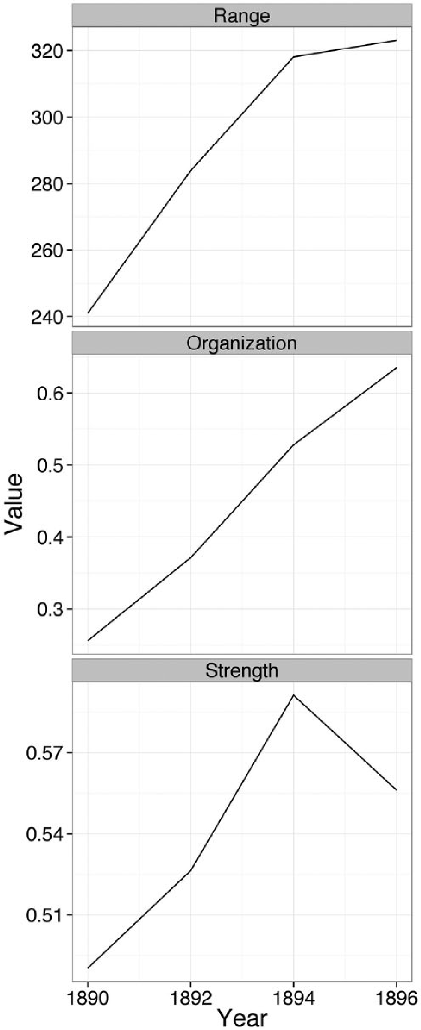
Changes in field measures for data in Figure 3.

Indeed, the turbulence visible in the Minneapolis–St. Paul area makes sense given the centrality of the Twin Cities in the trade network associated with production, exchange, and processing of grain, with wheat in particular emerging as the region’s most dominant crop. The two cities were also situated between two very different socioeconomic regions. Whereas southeastern Minnesota had a large German-born population, the area to the area to the northwest of the city featured a sizable Scandinavian population. There was a similar division with respect to agriculture. Unlike the case of the southeast where farmers had already made the turn toward diversified agriculture, farmers in the northwest tended to focus on the production of wheat. In light of our ability to capture substantively meaningful trends, we believe that visual inspection of graphs such as the ones above may be of great use in identifying otherwise unknown points of abrupt change in field effects.

Two Examples with Multiple Vectors and Individual-level Data

We saw earlier encouraging provisional results from a technique that began by assuming the presence of a particular form of spatial autocorrelation—the same form assumed by all techniques that attempt to deal with spatially situated data—whereby the correlation between two places near is greater than that between places far. This is, as noted above, is the basic intuition behind Tobler’s first law, which is ubiquitous in the field of geography. We go on to argue that this assumption is indeed a reasonable one for most cases but that there are times when this assumption breaks down. Fortunately, our measures still produce interpretable results when other patterns of alignment hold. Furthermore, although example 1 used ecological data (and therefore used convenient assumptions for purposes of illustration), our measures are in no way restricted to such cases. In the discussion below, we show how these same measures can be used to analyze data in the form of individuals nested within places. We also introduce a somewhat different way of investigating the alignment function.

Vectors from Individual-level Data

For example 2, we take data in which multiple individuals are nested within a geographic position, allowing us to compute our vectors by carrying out conventional regressions within each position. We here derive our measures from a large set of data on voting behavior collected by the firm Polimetrix (Ansolabehere 2011). We focus in particular on voting in the continental United States in 2008. With an overall N of 32,800, we have enough cases to run separate models for each congressional district, as well as for the District of Columbia. More specifically, we use linear regression to estimate the relationship between party identification (a seven-point scale running from “strong Democrat” [1] to “strong Republican” [7]), income, education, and race, with party identification serving as the outcome. We therefore have three different vectors, one for each independent variable.¹³

Specification of the Vectors and Alignment Function

In this case, we may decide that rather than choose one vector, we may want to use more than one to determine the general alignment between positions so as to better estimate the similarity across places.

More generally, for every area i, we estimate a set of M multiple regression slope parameters β_i = (β_i1, β_i2, β_i3, . . . β_iM). The usual question of how to compare slopes arises in this case; here we will assume that we standardize our slopes so that they are in terms of unit variances. We now wish to determine the g_ij between any two areas. We might reasonably propose again to use the dot-product-based correlation

g_{i j} = \cos θ = \frac{β_{1} \cdot β_{2}}{‖ β_{1} ‖ ‖ β_{2} ‖},

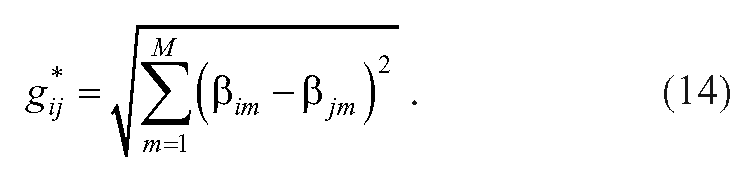
though one will note that this is actually different in form from the earlier equation 12. That is, equation 12 is not a special case of equation 13.¹⁴ However, equation 13 turns out not to be substantively reasonable measure of the alignment. Consider two cases with slopes observed on four variables as follows: β_i = [1, 0, –2, 3] and β_j = [.5, 0, –1, 1.5]. The correlation between the two is 1.0, in that β_im = 2β_jm for all m. Yet we should not consider these interchangeable situations. Thus instead of standardizing in the usual way—so that we lose all difference in absolute scaling in order to concentrate on relative differences—we are actually interested in the absolute difference between any two vectors. Accordingly, consider the measure of the distance between the tips of these vectors in the multidimensional space of independent variable slopes:

g_{i j}^{*} = \sqrt{\sum_{m = 1}^{M} {(β_{i m} - β_{j m})}^{2}} .

Unlike the single-vector measure (equation 12), the measure above lacks interpretable bounds.¹⁵ As a reasonable ad hoc adjustment, we propose

g_{i j} = \frac{g *_{\max} - 2 g *_{i j}}{g *_{\max}},

where

g *_{\max} = \max (g *_{i j}) .

This approach seems to be relatively robust and interpretable, especially for examining a single data set. But because the normalizing is specific to each data set, in that the maximum correlation may differ from one data set to the next, it can be difficult to examine change or difference. In such cases, it may be preferable to use the maximum across all relevant data sets for purposes of comparability. Finally, here we use geographic distance between centroids of congressional districts as our distance (equation 7) and, for each district, use the set of three slope coefficients as our vector β_i, and equation 15 to measure the alignment between districts.

Alignment and Space

Figure 6 displays a smoothed moving average of the alignment function by distance akin to the hypothetical curve graphed in Figure 2. We see that overall, there is indeed evidence that the alignment decreases with distance. From 25 to 2,500 miles, we see a close approximation to Figure 2. However, things change dramatically at the very great and the very small distances. Places that are extremely far apart turn out to be more likely to be similar, not less likely, than average pairs of places.

Figure 6.

Autocorrelation pattern for all congressional districts in the contiguous 48 states of the United States, 2008.

This is because as a result of the doctrine of manifest destiny, the United States has the enviable position of occupying a nice horizontal swath of a continent with two large vertical coasts facing different oceans. Although the denizens of these areas are not wholly interchangeable, there is (as any midwesterner can aver) something decidedly similar about “coasties,” whether they hail from the “east” or the “left” coast. Thus although the 48 contiguous states of the United States look vaguely like a rectangle, in social terms it is perhaps more like a cylinder that we would form were we to detach the country from the earth and join Portland, Maine, to Portland, Oregon, at the top, while overlaying Disneyland and Disneyworld at the bottom.

The other reversal comes at very close range—congressional districts very close to one another are surprisingly unlike. The reason for this lies, we believe, with the social organization of American cities, especially their segregated nature. The only places where districts are so close together are in metropolitan areas, and metropolitan areas divide people up—and even where they do not, congressional districts may be deliberately drawn to place “similar” people on similar sides of the boundary.¹⁶

Figure 7 demonstrates this using data from the US Census Bureau’s 2008 American Community Survey. For each of these graphs, we grouped pairs of districts into bins of 1,000 (ordered by geographic distance), then plotted the mean absolute value of the difference between the districts on each of a set of measures by the mean geographic distance for all pairs in that bin. We look at the (absolute value of the) difference between districts in terms of four indicators of the “type” of place, namely, the percentage of structures for dwelling that are one family, the median household income, the poverty rate, and the proportion of residents who are high school graduates. For two of the indicators (income and education), we see a very typical spatial organization in which, if we start with the farthest pairs, we find that distant places are very different, and differences decrease as places get closer; though as we near the 25- to 50-mile mark, differences increase dramatically. For poverty and one-family structures, there is hardly any spatial organization except that places become very dissimilar as they get extremely close (and for one-family structures, extremely far).

Figure 7.

The spatial organization of inequality in cities leads to differences among close districts.

It is important to realize that it is entirely possible for places to be very different with respect to average income, say, while the slope of party identification regressed on income is constant. Indeed, that is what we generally assume when we use a conventional linear model. But we are finding that changes in the distribution of the independent variable are associated with changes in the relation between the independent and dependent variables and that this is happening in a way related to the spatial organization of the United States.

On the whole, the conclusion here is not that Tobler’s law is wrong but that we may expect a change in sign in the nature of alignment for a number of indicators of social and political organization, whereby an increasing similarity with geographic proximity, past some threshold turns into a decreasing similarity with proximity, if we are approaching an urban area. If we increase our focus even further, we may again see a reversal of sign at the block level, but our data do not permit us this exploration. To return to Park (1926) and Koffka (1935), we must bear in mind that the effects of geographic space are mediated by social organization and perception.

As a result, there is no reason why we cannot begin to generalize our approach to distances, even distances in geographic space, that are defined not by crow’s-flight distance, but by political interconnection (Beckfield 2010), telecommunication patterns (Louch, Hargittai, and Centeno 1999) or transportation times. Whatever form of “distance” has social effects is the one that is most important for the measurement of field strength.

Change in Field Strength

We have seen evidence that the assumptions underlying the measurement strategy here seem reasonably robust, though there are likely to be cases in which these assumptions are violated, and there is no substitute for substantive knowledge of the social processes in question. But it is also worth emphasizing that the validity of the measurement strategy outlined here is not conditional on the data following the sort of pattern seen in Figure 2; the overall range of order, say, still can be informative where the pattern is quite different.

And the measurement strategy here may be of great use when our interest is in exploring changes in the organization of some field over time. In the future, large-scale data sets like that used in the previous section will allow a direct extension of the methods used here, but for most of the twentieth century, our individual-level data sets have smaller totals that make such a complete investigation impossible. Yet it may be possible, through judicious use of pooling and various benign assumptions, to make use of other sets of data.

As an example (example 3), we analyze data from the American National Election Studies, which were conducted using a national sampling frame from 1956 until the present. Surveys were usually carried out every two years (sometimes gaps of four years occurred between studies). We examine variation in patterns of votes for Congress between 1956 and 2004, analyzing congressional districts separately. However, in many cases, we do not have sufficient numbers of persons from particular districts to allow models to be fit in those districts. We therefore use an algorithm that pools across close places and close times, in order to maximize the number of valid data points.¹⁷ We fit models that simultaneously control for income, education, and race. Using this, we can then create our field measures). Here, we are particularly interested in the range of the income effect. Thus, as in example 2, our vectors are multiple regression slopes, but as in example 1, we compute our alignment function only using one vector (equation 12). Again, we use geographic distance as in the previous examples.

The range of the income effect is displayed in Figure 8, running from 1960 to 2000 (because of our moving average, we have no data points before or after this period). We see a steady creeping upward of the range, such that about 200 miles have been added by the end of the twentieth century. That is, places that were 1,100 miles apart in 2000 were about as similar in terms of their income effect as places 900 miles apart were 40 years before. Our example is merely illustrative of the logic of the technique, and is not intended as a strong theoretical statement. But the gradual linear increase, and the independence of the results from changes in the sampling frame, leads us to believe that this approach can be made robust and lend itself to temporal investigations.

Figure 8.

Change in range of income over the second half of the twentieth century, National Election Studies.

One Example of Individuals in a Social Space

Vectors and Alignment

In example 1, we began by considering ecological data in physical space. This approach is fairly natural in the sense that the units of analysis are explicitly defined in spatial terms. As we showed in example 2, however, the field theoretic measures proposed above can be easily applied to individual data as well. Although we relaxed the assumption that that the original data are composed of ecological entities, we nonetheless maintained our focus on physical space, in that the individuals in question were nested in areal units that were then used to geolocate the resulting vectors. Note, however, that the measures themselves are in no way limited to the case of physical space. As we show here, the methods outlined above can be easily extended to accommodate distance in social space.

This returns us to issues with which we began. As we noted, most prior attempts to quantify field effects have relied upon CA and the interpretation of its estimates as yielding positions in a multidimensional social space. It is certainly possible to use these derived positions in conjunction with the measures proposed here. For those who are suspicious of tautological techniques such CA that create a “space” for every set of data, we outline an alternative procedure on the basis of the notion of Blau space, first introduced by McPherson and Ranger-Moore (1991). The basic intuition behind this approach is that we can construct a multidimensional space by simply cross-classifying variables, with the dimensionality of the resulting space equal to the number of variables considered. In the absence of any further data reduction, the dimensions are given rather than derived, thus avoiding some of the thornier issues associated with CA and related techniques such as factor analysis and multidimensional scaling.

To illustrate this approach, we used the General Social Survey cumulative data file to construct spaces of likeness for 57,000 respondents, with dimensions defined in terms of age (with categories 18–29, 30–38, 39–59, 50–62, and 63–89 years), sex (two categories), and size of community (with categories standard metropolitan statistical area, one of the 12 largest suburbs, other suburbs of large standard metropolitan statistical area, small cities, and rural). Within each area of this 5 × 2 × 5 social space, we separately regress presidential vote on occupational prestige. Thus we construct vectors just as we did in examples 2 and 3 and use a single-vector alignment measure (equation 12), just was we did in examples 1 and 3.

Distance

In the context of a tautological-space approach such as CA, the definition of distance is relatively unproblematic, in that the resulting statistic is effectively unitless.¹⁸ In the case of Blau space, on the other hand, we are faced with the problem that our dimensions are in different units by virtue of the fact that the variables used to define those dimensions are themselves in different units. To determine distance in this space, we rescale each of the variables to have a standard deviation of 1, thus assigning an equal weight to each. We then calculate the Euclidean distance between all positions.

Field Effects

In this case, we use the field measures to assess the degree to which the same variables, stimuli, or conditions provoke similar vectors in different areas of this space, and our measures are measures of the degree of organization in this social space. For the purposes of examining change over time, we begin by breaking the data into two periods: 1981 to 2000 and 2001 to 2012. Running a separate analysis for each period, we observe an increase in both the organization and strength of the field. More specifically, in the case of organization (F; equation 5), we observe a rise from 0.628 to 0.706 (recall that organization is measured on a scale from 0 to 1). In the case of strength (S; equation 6), on the other hand, we observe a rise from 26.05 to 31.15. Given that the difficulty associated with interpreting this particular measure of strength (as it is in the metric of “logit per standard deviation of prestige”), we might dismiss this as meaningless noise. But the same direction is seen when we look more finely.

We repeat the exercise above, this time breaking our data up into eight four-year periods (1981–1984; 1985–1988; 1989–1992; 1993–1996; 1997–2000; 2001–2004; 2005–2008 and 2009–2012). (We chose this periodization because we wanted to make sure we did not pool respondents who would be facing different presidential contests.) Figure 9 displays the results: we see that there has been a constant increase in the organization of the field, with a very large increase in the most recent period. This suggests that given the structure of the underlying space, there has been a trend toward more organization and more similarity in how prestige impels voting choices. This example, whether or not it is substantively compelling in its own right, demonstrates the possibility of the use of these measures to make interpretable claims about fields that are organized in social, not geographic, space.

Figure 9.

Change in field organization (F) over time, social space.

Conclusion

To steal Samuel Johnson’s words, the marvel of the field analysis, like that of a dog walking on its hind legs, is not that it is done particularly well, but just that it can be done at all. The methods discussed here are rudimentary. They are descriptions that allow limited comparison across different questions. However, this is generally true in the social sciences. It is only through habit that we imagine that a correlation of .4 means the same thing in one data set that it does in another. Even more, in sociology we usually replace any understanding of descriptive accuracy with an altogether different question of statistical significance, which avoids the problem of comparison entirely.

Thus the fact that the measures here are limited is not in itself a fatal flaw. More important is the fact that they take the intuition underlying many field analogies, that of the alignment of vectors and demonstrate that this can lead to a set of measurement strategies that are not the same as existing strategies. These strategies make sense when there is good reason to believe that a field of a certain type exists. They will not replace other descriptive statistics that do not have such substantive requirements. But we do believe that there is an important role for model-independent descriptions of the various dimensions of a given field effect in our panoply of techniques for learning from data.

Furthermore, with such descriptions, the more we know about the dynamics of the field in question, the more we may adapt the approach here to take into account our substantive understanding. Certainly, we can move to spaces of higher dimension or with particular types of curvature. We can also incorporate directionality, as opposed to considering all distances symmetric and space isotropic (Oden and Sokal 1986). And we can even meld the continuous spaces with discontinuous organizational locations. Simple geographic distances, such as arise when we have action located in places like counties or congressional districts, are indeed a good place to start if we wish to develop a measurement approach, but we need not stay on the surface of the Earth. If indeed “social space” (Sorokin [1927] 1959) deserves to be treated as more than a metaphor, we should be able to pursue similar analyses in which our vectors are organized by their position in this space.

Footnotes

Appendix A: Details on Geographic Data

Acknowledgements

We are grateful for the support of Henry Brady, Neil Fligstein, Jacob Foster, Eric Oliver, Loïc Wacquant, and of course Harrison White and for the criticisms of the reviewers, which pushed us to explore certain complications.

Authors’ Note

Earlier versions of this article were presented at the University of California, Berkeley, Survey Research Center Occasional Papers Colloquium, at the Princeton University Department of Sociology, at the University of Chicago American Politics Workshop, and a at special conference on measuring social fields at the University of California, Berkeley. Software available at https://www.github.com/aslez/femar and replication files at .

Notes

Author Biographies

John Levi Martin is the Florence Borchert Bartling Professor of Sociology at the University of Chicago. He is the author of Social Structures, The Explanation of Social Action, and Thinking Through Theory, as well as articles on methodology, cognition, social networks, and theory. He is currently working on the history of the theory of social action.

Adam Slez is an assistant professor in the Department of Sociology at the University of Virginia. Using spatial data analysis along with more traditional forms of historical inquiry, his recent work examines the way in which policies related to the expansion of the railroad network contributed to patterns of third-party mobilization in the American West over the course of the late nineteenth century. His previous work on state and party formation in the United States Constitutional Convention of 1787 has appeared in the American Sociological Review.

Chad Borkenhagen is a PhD candidate in sociology at the University of Chicago. His research interests include organizations, culture, knowledge, status, and creativity. His dissertation examines the growing role of scientific knowledge in the traditionally nonscientific fields of finance and the culinary arts.

References

Achen

Christopher H.

Shively

W. Phillips

. 1995. Cross-level Inference. Chicago: University of Chicago Press.

Anselin

Luc

. 1988. Spatial Econometrics: Methods and Models. Dordrecht, the Netherlands: Kluwer Academic.

Anselin

Luc

. 1995. “Local Indicators of Spatial Association—LISA.” Geographical Analysis 27(1):93–115.

Anselin

Luc

Cho

Wendy K. Tam

. 2002. “Spatial Effects and Ecological Inference.” Political Analysis 10(3):276–97.

Ansolabehere

Stephen.

2011. “Cooperative Congressional Election Study, 2008: Common Content.” Release 3. Cambridge, MA: Harvard University.

Armstrong

Elizabeth A.

2002. Forging Gay Identities: Organizing Sexuality in San Francisco, 1950–1994. Chicago: University of Chicago Press.

Baker

F. B.

Hubert

L.J.

1981. “The Analysis of Social Interaction Data: A Nonparametric Technique.” Sociological Methods and Research 9(3):339–61.

Barman

Emily

. 2007. “An Institutional Approach to Donor Control: From Dyadic Ties to a Field-level Analysis.” American Journal of Sociology 112(5):1416–57.

Beckfield

Jason

. 2010. “The Social Structure of the World Polity.” American Journal of Sociology 115(4):1018–68.

10.

Benzécri

J. P.

1991) “Measures, Models, and Graphical Displays in the Analysis of Cross-classified Data: Comment.” Journal of the American Statistical Association 86(416):1112–14.

11.

Berman

Elizabeth Popp

. 2006. “Before the Professional Project: Success and Failure at Creating an Organizational Representative for English Doctors.” Theory and Society 35(2):157–91.

12.

Blalock

Hubert M.

1964. Causal Inferences in Nonexperimental Research. Chapel Hill: University of North Carolina Press.

13.

Bourdieu

Pierre

. [1966] 1969. “Intellectual Field and Creative Project.” Social Science Information 8(1):89–119.

14.

Bourdieu

Pierre

. [1979] 1984. Distinction: A Social Critique of the Judgment of Taste. Translated by Nice

Richard

. Cambridge, MA: Harvard University Press.

15.

Bourdieu

Pierre

. [1984] 1988. Homo Academicus. Translated by Collier

Peter

Stanford, CA: Stanford University Press.

16.

Bourdieu

Pierre

Wacquant

Loïc J. D.

1992. An Invitation to Reflexive Sociology. Chicago: University of Chicago Press.

17.

Breder

C. M.

Jr.

1951. “Studies on the Structure of the Fish School.” Bulletin of the American Museum of Natural History 98, Article 1.

18.

Breder

C. M.

Jr.

1954. “Equations Descriptive of Fish Schools and Other Animal Aggregations.” Ecology 35(3):361–70.

19.

Breiger

Ronald L.

2000. “A Tool Kit for Practice Theory.” Poetics 27:91–115.

20.

Brunsdon

Chris

Fotheringham

Stewart

Charlton

Martin

. 1998. “Geographically Weighted Regression—Modelling Spatial Non-stationarity.” Statistician 47(3):431–43.

21.

Butts

Carter T

. Forthcoming. Space and Structure: Methods and Models for Large-scale Interpersonal Networks. New York: Springer.

22.

Calvo

Ernesto

Escolar

Marcelo

. 2003. “The Local Voter: A Geographically Weighted Approach to Ecological Inference.” American Journal of Political Science 47(1):189–204.

23.

Cavagna

Duarte Queirós

S. M.

Giardina

Stefanini

Viale

2013. “Diffusion of Individual Birds in Starling Flocks.”

Proceedings of the Royal Society B

280:20122484.

24.

Cavalli-Sforza

L. Luca

Menozzi

Paolo

Piazza

Alberto

. 1994. The History and Geography of Human Genes. Princeton, NJ: Princeton University Press.

25.

Chaix

Basile

Merlo

Juan

Subramanian

S. V.

Lynch

John

Chauvin

Pierre

. 2005. “Comparison of a Spatial Perspective with the Multilevel Analytic Approach in Neighborhood Studies: The Case of Mental and Behavioral Disorders Due to Psychoactive Substance Use in Malmö, Sweden, 2001.” American Journal of Epidemiology 162(2):171–82.

26.

Clark

W. A. V.

Avery

Karen L.

1976. “The Effects of Data Aggregation in Statistical Analysis.” Geographical Analysis 8:428–38.

27.

Couzin

Iain D.

2003. “Self-organization and Collective Behavior in Vertebrates.” Advances in the Study of Behavior 32(1):1–75.

28.

Evans

Rhonda

Kay

Tamara

. 2008. “How Environmentalists ‘Greened’ Trade Policy: Strategic Action and the Architecture of Field Overlap.” American Sociological Review 73(6):970–91.

29.

Ferguson

Priscilla Parkhurst

. 1998. “A Cultural Field in the Making: Gastronomy in 19th-century France.” American Journal of Sociology 103(3):597–641.

30.

Fligstein

Neil

McAdam

Doug

. 2012. A Theory of Fields. New York: Oxford University Press.

31.

Fotheringham

A. S.

Wong

D.W.S.

1991. “The Modifiable Areal Unit Problem in Multivariate Statistical Analysis.” Environment and Planning A 23(7):1025–44.

32.

Fotheringham

A. Stewart

Brunsdon

Chris

Charlton

Martin

. 2002. Geographically Weighted Regression: The Analysis of Spatially Varying Relationships. West Sussex: John Wiley & Sons, Ltd.

33.

Gehlke

C. E.

Biehl

Katherine

. 1934. “Certain Effects of Grouping upon the Size of the Correlation Coefficient in Census Tract Material.” Journal of the American Statistical Association 29:169–70.

34.

Gelman

Andrew

Shor

Boris

Bafumi

Joseph

Park

David

. 2007. “Rich State, Poor State, Red State, Blue State: What’s the Matter with Connecticut?” Quarterly Journal of Political Science 2(4):345–67.

35.

Ginelli

Francesco

Peruani

Fernando

Pillot

Marie-Helène

Chaté

Hugues

Theraulaz

Guy

Bon

Richard

. 2015. “Intermittent Collective Dynamics Emerge from Conflicting Imperatives in Sheep Herds.”

Proceedings of the National Academy of Sciences

112(41):12729–34.

36.

Julian

. 2008. “Global Fields and Imperial Forms: Field Theory and the US and British Empires.” Sociological Theory 26(3):201–29.

37.

Goodman

Leo

. 1953. “Ecological Regression and the Behavior of Individuals.” American Sociological Review 18(6):663–64.

38.

Goodman

Leo A.

1959. “Some Alternatives to Ecological Correlation.” American Journal of Sociology 64(6):610–25.

39.

Griffith

Daniel A.

2008. “Spatial-Filtering-Based Contributions to a Critique of Geographically Weighted Regression (GWR).” Environment and Planning A 40:2751–69.

40.

Haveman

Heather A.

Rao

Hayagreeva

Paruchuri

Srikanth

. 2007. “The Winds of Change: The Progressive Movement and the Bureaucratization of Thrift.” American Sociological Review 72(1):114–142.

41.

Hipp

John R.

Faris

Robert W.

Boessen

Adam

. 2012. “Measuring ‘Neighborhood’: Constructing Network Neighborhoods.” Social Networks 34(1):128–40.

42.

Hubert

1985. “Combinatorial Data Analysis: Association and Partial Association.” Psychometrika 50(4):449–67.

43.

Hubert

Schultz

1976. “Quadratic Assignment as a General Data Analysis Strategy.” British Journal of Mathematical and Statistical Psychology 29(2):190–241.

44.

King

Gary

. 1997. A Solution to the Ecological Inference Problem. Princeton, NJ: Princeton University Press.

45.

Koffka

Kurt

. 1935. Principles of Gestalt Psychology. New York: Harcourt, Brace.

46.

Köhler

Wolfgang

. 1920. Die physichen Gestalten in Ruhe und im stationären Zustand. Braunschweig, Germany: Vieweg und Sohn.

47.

Köhler

Wolfgang

. 1947. Gestalt Psychology. New York: Liveright.

48.

Krackhardt

1987. “QAP Partialling as a Test of Spuriousness.” Social Networks 9(2):171–86.

49.

Krackhardt

1988. “Predicting with Networks: Nonparametric Multiple Regression Analysis of Dyadic Data.” Social Networks 10(4):359–81.

50.

Krackhardt

1992. “A Caveat on the Use of the Quadratic Assignment Procedure.” Journal of Quantitative Anthropology 3(4):279–96.

51.

Laiolo

Paola

. 2008. “Characterizing the Spatial Structure of Songbird Cultures.” Ecological Applications 18(7):1774–80.

52.

Lewin

Kurt

. 1951. Field Theory in Social Science. Edited by Cartwright

Dorwin

. New York: Harper.

53.

Louch

Hugh

Hargittai

Eszter

Centeno

Miguel Angel

. 1999. “Phone Calls and Fax Machines: The Limits to Globalization.” Washington Quarterly 22(2):83–100.

54.

Lounsbury

Michael

Ventresca

Marc

Hirsch

Paul

. 2003. “Social Movements, Field Frames and Industry Emergence: A Cultural-political Perspective on U.S. Recycling.” Socio-economic Review 1(1):71–104.

55.

Mantel

Nathan

. 1967. “The Detection of Disease Clustering and a Generalized Regression Approach.” Cancer Research 27(2):209–220.

56.

Markoff

John

Shapiro

Gilbert

. 1973. “The Linkage of Data Describing Overlapping Geographical Units.” Historical Methods Newsletter 7:34–46.

57.

Martin

John Levi

. 2003. “What Is Field Theory?” American Journal of Sociology 109(1):1–49.

58.

Maxwell

James Clerk

. [1891] 1954. A Treatise on Electricity and Magnetism. New York: Dover.

59.

McPherson

J. Miller

Ranger-Moore

James

. 1991. “Evolution on a Dancing Landscape: Organizations and Networks in Dynamic Blau Space.” Social Forces 70(1):19–42.

60.

Moran

P.A.P.

1950. “Notes on Continuous Stochastic Phenomena.” Biometrika 37(1):17–23.

61.

Morenoff

Jeffrey D.

2003. “Neighborhood Mechanisms and the Spatial Dynamics of Birth Weight.” American Journal of Sociology 108(5):976–1017.

62.

Oden

Neal L.

Sokal

Robert R.

1986. “Directional Autocorrelation: An Extension of Spatial Correlograms to Two Dimensions.” Systematic Zoology 35(4):608–617.

63.

Openshaw

Stan

. 1983. The Modifiable Areal Unit Problem. Norwich: Geo Books.

64.

Openshaw

Stan

Taylor

Peter J.

1979. “A Million or So Correlation Coefficients: Three Experiments on the Modifiable Areal Unit Problem.” Pp. 126–44 in Statistical Applications in the Spatial Sciences, edited by Wrigley

London: Pion Limited.

65.

Park

Robert E.

1926. “The Concept of Position in Sociology.” Papers and Proceedings of the American Sociological Society 20:1–14.

66.

Park

Robert E.

Burgess

Ernest W.

McKenzie

Roderick D.

[1925] 1967. The City. Chicago: University of Chicago Press.

67.

Parrish

Julia K.

Turchin

Peter

. 1997. “Individual Decisions, Traffic Rules, and Emergent Patterns in Schooling Fish.” Pp. 126–42 in Animal Groups in Three Dimensions, edited by Parrish

Julia K.

Hamner

William M.

Cambridge, UK: Cambridge University Press.

68.

Quinn

Sarah

. 2008. “The Transformation of Morals in Markets: Death, Benefits, and the Exchange of Life Insurance Policies.” American Journal of Sociology 114(3):738–80.

69.

Rawlings

Craig M.

Bourgeois

Michael D.

2004. “The Complexity of Institutional Niches: Credentials and Organizational Differentiation in a Field of US Higher Education.” Poetics 32(6):411–37.

70.

Ray

Raka

. 1999. Fields of Protest: Women’s Movements in India. Minneapolis: University of Minnesota Press.

71.

Reardon

Sean F.

Farrell

Chad R.

Matthews

Stephen A.

O’Sullivan

David

Bischoff

Kendra

Firebaugh

Glenn

. 2009. “Race and Space in the 1990s: Changes in the Geographic Scale of Racial Residential Segregation, 1990–2000.” Social Science Research 38(1):55–70.

72.

Reardon

Sean F.

O’Sullivan

David

. 2004. “Measures of Spatial Segregation.” Sociological Methodology 34(1):121–162.

73.

Robinson

W. S.

1950. “Ecological Correlations and the Behavior of Individuals.” American Sociological Review 15(3):351–57.

74.

Schabenberger

Oliver

Gotway

Carol A.

2005. Statistical Methods for Spatial Data Analysis. New York: Chapman & Hall/CRC Press.

75.

Slez

Adam

. 2011. “The Changing Context of Electoral Politics in the American West, 1861–1896.” Unpublished PhD dissertation. Madison: University of Wisconsin.

76.

Slez

Adam

O’Connell

Heather A.

Curtis

Katherine J.

Forthcoming. “A Note on the Identification of Common Geographies.” Sociological Methods and Research.

77.

Sorokin

Pitirim A.

[1927] 1959. Social and Cultural Mobility. Glencoe, IL: Free Press.

78.

Tobler

Waldo

. 1970. “A Computer Movie Simulating Urban Growth in the Detroit Region.” Economic Geography 46(2):234–240.

79.

Wheeler

David

Tiefelsdorf

Michael

. 2005. “Multicollinearity and Correlation among Local Regression Coefficients in Geographically Weighted Regression.” Journal of Geographic Systems 7(2):161–87.

80.

Wheeler

David C.

Waller

Lance A.

2009. “Comparing Spatially Varying Coefficient Models: A Case Study Examining Violent Crime Rates and Their Relationships to Alcohol Outlets and Illegal Drug Arrests.” Journal of Geographical Systems 11:1–22.

81.

White

Harrison C.

1992. Identity and Control. Princeton, NJ: Princeton University Press.

82.

Ziman

J.M.

1979. Models of Disorder: The Theoretical Physics of Homogeneously Disordered Systems. Cambridge, UK: Cambridge University Press.

Some Provisional Techniques for Quantifying the Degree of Field Effect in Social Data

Abstract

Keywords

An Approach to Measuring Fields

Overall Logic

The Sociology of Space

Fields as Correlation Structures

Quantifying Field Effects

The Autocorrelation Function and Field Effect

Measures of Field Organization and Strength

Geographic Fields with Single Vectors

The Case and Definition of Vectors

The Distance Function

Alignment Functions for Single Vectors

Changes in the Field

Two Examples with Multiple Vectors and Individual-level Data

Vectors from Individual-level Data

Specification of the Vectors and Alignment Function

Alignment and Space

Change in Field Strength

One Example of Individuals in a Social Space

Vectors and Alignment

Distance

Field Effects

Conclusion

Footnotes

Appendix A: Details on Geographic Data

Acknowledgements

Authors’ Note

Notes

Author Biographies

References