Window dressing in the Active Share scores in publicly reported portfolios

Abstract

Using a unique database that includes publicly disclosed fund holdings at the end of the quarter as well as the holdings in all non-publicly disclosed months, we found that some funds could alter their portfolios in publicly disclosed months to artificially increase their Active Share scores and consequently appear more active and take advantage of the positive relationship between Active Share and money flows. We show how, consistent with non-informed trades, these funds erode their future performance. However, these funds reach their objective of increasing future money flows. Moreover, we find that window-dresser funds can be identified by controlling the level of tracking error. The funds with high Active Share scores and low tracking errors have the highest levels of Active Share window dressing and the worst future returns. However, compared with less active funds, they are able to capture higher money flows.

JEL CLASSIFICATION G23; G11

Introduction

The existence of window dressing (WD) in portfolio management has attracted increasing interest among academics and practitioners because of its managerial consequences. Previous literature describes WD as a management strategy intended to include attractive assets (hot stocks) and/or prevent unattractive assets in the reported portfolios to draw higher money flows. Different measures have been proposed to capture this phenomenon, depending on the reasons for WD behavior (see Agarwal et al., 2014).

In this study, we analyze a different type of WD where managers attempt to increase the difference in the portfolio weights between their reported portfolio and the benchmark. Actively managed funds offer portfolios that attempt to outperform a reference benchmark by actively deviating from the benchmark weights overweighting (underweighting) the stocks that the manager considered good (bad) investments. Active mutual funds charge higher fees for this active management. Moreover, investors could consider large deviations from the benchmark a proxy for skill and consequently indicate higher probabilities for better future performance. Therefore, we suggest that fund managers could be tempted to artificially increase the deviation of their portfolio weights from the benchmark weights in the months when their portfolio holdings are made public to give an extra image of activeness. With this WD strategy, managers could better justify their high fees and also portray a higher image of skill to potential investors, which could consequently increase their money flows.

We use the Active Share (AS) measure proposed by Cremers and Petajisto (2009) as an aggregate measure of how fund holdings deviate from the benchmark. This measure adds the absolute value of all the fund stock weight deviations from the benchmark weights. Although the work of Cremers and Petajisto (2009) was published after our sample period (2000–2006), the AS metric is so intuitive that we consider it a good proxy of how investors compute aggregate fund holding deviations from the benchmark in the sample period.

“Hot stocks” and “AS” WD practices refer to portfolio holding movements before the fund portfolio becomes public with the same final objective of increasing money flows. However, they are different. Note that when “hot stocks” WD managers buy (sell) attractive (unattractive) stocks, which are overweighted (underweighted) in the portfolio, this trade will necessarily increase stock deviation from benchmark, and therefore increase AS levels. However, when “hot stocks” WD managers buy (sell) attractive (unattractive) stocks which are underweighted (overweighted) in the portfolio, this trade could reduce the stock deviation from benchmark, and therefore reduce AS levels.

To compute AS WD, it is necessary to have a database that includes fund holdings both in the months during which the fund portfolios are made public to investors and the months during which these fund portfolios are not made public. We employ a unique database for the Spanish mutual fund market that includes both publicly disclosed fund holdings at the end of the quarter (March, June, September, or December) and the fund holdings in all non-publicly disclosed months (non-quarter-end months). This information is not publicly available to investors as the Spanish official supervisor provides non-quarter-end fund holdings for research purposes only. This makes this database especially useful for our aim. Moreover, this database is free of any selection bias, given that this information is available to all mutual funds and is provided by the official supervisor rather than a private supplier.

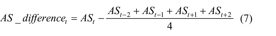
The quality of the information available in the Spanish market allows us to detect the potential WD in the AS levels in publicly reported months, as we can compute how the AS in public quarter-end months differs from the AS in the two previous and the following two non-public months. We refer to this AS WD proxy as AS_difference. This study cannot be extended to other eurozone markets. ¹ However, our results are relevant to the worldwide mutual fund industry. Cremers and Petajisto (2009) argue that AS scores based on reported fund holdings at the end of a quarter are unlikely to suffer any potential WD because the portfolio distortion supposes a high turnover cost. However, evidence of AS WD in the Spanish mutual fund market would mean that fund managers worldwide could have enough incentives to alter their portfolios despite the turnover costs. Moreover, the Spanish domestic mutual fund market exhibits some characteristics (small size of the Spanish Stock Exchange) that make it difficult for managers to deviate from the benchmark. If Spanish managers find enough incentives to alter their AS despite the difficulties of deviating from the benchmark, managers from other countries with fewer difficulties could have even more incentives to window dress the level of AS.

This study’s main contribution is testing, for the first time in literature, whether mutual funds alter their holdings in publicly disclosed months to appear more active and how this WD strategy influences future fund performance and money flows. We also contribute to the WD literature by examining the undisclosed information. Few studies (e.g., Elton et al., 2010; Morey & O’Neal, 2006; Musto, 1997; Ortiz et al., 2012) are able to use both disclosed and undisclosed information. However, in most cases, there exists some reporting selection bias.

In our study, the incentives to alter AS in publicly reported months depend on whether the AS score is positively related to the future performance of fund (manager skills) and future money flows. In the first part of the study, we demonstrate that the higher the AS level, the higher the future fund returns and money flows. Moreover, we also investigate whether this relation is robust for the inclusion of tracking error (TE) as an alternative measure of fund activeness.

If some managers alter their AS levels, they will increase this measure before publicly disclosed months and revert to their previous levels afterward. In this case, managers deviate the portfolio holdings from the benchmark only to offer a temporal higher level of activeness when they are going to make the information public, and not because the manager is overweighting (underweighting) stocks that, according to the manager’s skill, are going to be winners (losers). This AS increase is artificial and not related to skill. In addition, if AS is a proxy for management skills, the skills should not differ between publicly and non-publicly disclosed months. Therefore, this WD strategy will erode fund performance because of the increase in turnover and expense ratios. However, if some managers decide to modify the AS level despite its expected negative impact on fund performance, it would be because this practice allows for future money flows to increase. Consistent with this idea, we find that high levels of AS in publicly reported months regarding the AS levels in the two previous and the following two non-publicly reported months (AS_difference) are related to worse future fund performance and better future money flows.

Our analysis also focuses on detecting funds that are more likely to distort the AS level. Given that TE cannot be modified easily, we suggest that funds with high AS but low TE levels are more likely to alter their AS levels. We consistently find that contrary to the other categories of funds, on average, funds with high AS but low TE levels increase their AS levels before their holdings are made public and reduce them afterward. They therefore show significant and positive AS_difference values. Moreover, this category of funds shows the worst future performance but attracts higher money flows than funds with similar levels of TE.

Finally, given the findings of Golez and Marin (2015), who observe that Spanish bank-affiliated mutual funds systematically increase their holdings in the controlling bank stock around some events, we also analyze the possible AS WD strategies for subsamples of non-independent funds (funds managed by management companies that are integrated in a financial group conglomerate) and independent funds. We consistently find that the negative impact of AS WD at quarter-ends on fund performance is exclusive to non-independent funds. This negative impact is not observed in independent funds.

The rest of this article is organized as follows. The “Literature review and hypotheses” section presents the literature review and the hypotheses of the study. The “Data and measures” section describes the data and measures used in this study. The “Empirical models and methods” section describes the empirical models and methods used to test the hypotheses of this study. The “Main results” section presents the main findings of our hypotheses. The “Characteristics of stocks traded by AS window dressers: Is AS WD a practice different from ‘hot stock’ WD?” section examines the characteristics of stocks traded by AS window dressers. The section “Examining the funds that are more prone to window dress the AS level” examines the characteristics of funds that are more likely to alter the AS level. The “Robustness analyses” section presents some robustness analyses. The “Conclusion” section concludes the study.

Literature review and hypotheses

The information content in publicly disclosed fund holdings has attracted the interest of many studies. One important line of research, which is related to the existence of a conflict of interest between fund managers and investors, is the analysis of WD in fund holdings. Haugen and Lakonishok (1988) and Ng and Wang (2004) consider WD in fund holdings as the main factor that drives high returns for small and recent loser stocks after the year-end. Most studies examine the influence of this practice on price anomalies, such as the January effect, rather than examining the existence of this practice and its underlying motivations (see, for example, Agarwal et al., 2014). Specifically, Agarwal et al. (2014) highlight that there is limited understanding of the incentives for managers to engage in WD. They affirm that if WD is rewarded with higher flows, one might wonder why not all fund managers follow such activities. To disentangle this problem, these authors suggest that WD is a risky decision because its success in attracting higher flows depends on fund performance in the delay period between the end of the month when the portfolio is publicly disclosed and the date when this information is publicly disclosed to investors. ²

Hence, the main motivation for this practice is the perception of managers that portfolio disclosures significantly influence the opinions of investors regarding their professional skills. Managers are tempted to improve the appearance of their reported portfolio (i.e., including/deleting attractive/unattractive assets) before presenting them to clients or shareholders to attract larger money flows. The existence of WD is problematic for investors who seek reliable information on fund holdings that will help them allocate their money more appropriately.

Another line of research related to the information content in public fund holding disclosures uses these data to measure the level of active management and its relationship with fund performance. The first study to analyze this relation was Wermers (2003) which does not measure the level of active management using holding disclosures but uses return information through the TE. More recently, other studies have started analyzing active management using portfolio holdings information, which “a priori” provides a more comprehensive image of the activeness of portfolio managers. Kacperczyk et al. (2005) examined active management using portfolio concentration. More recently, Cremers and Petajisto (2009) analyzed how fund holdings deviate from benchmarks through the AS measure. These studies found a positive relationship between the level of active management and fund performance.

The AS measure has attracted substantial attention both in academia and in the management industry. Moreover, more active equity funds and institutional money managers currently report their AS. An example of this impact is the article published by Frazzini et al. (2016) which reviews the great impact of AS on the investment community. They indicate that institutional investors are more focused on asset managers with a high AS and that some institutional investors have even embedded a high AS requirement in their investment guidelines. Another example of the impact of AS in the fund community is Caquineau et al. (2016) from Morningstar, who advise investors not to rely solely on AS when selecting funds.

In this study, we link both lines of research (WD and active management) by examining a different practice of WD, that is, the report of a high level of differentiation from the benchmark on disclosure dates (AS WD) in the Spanish equity market. ³ Given that the incentives to distort the AS level depend on whether high AS levels in publicly reported portfolios send a positive signal to potential investors, we first analyze whether the US evidence of the effect of AS on future fund returns is observed in the Spanish market. Hence, our baseline hypothesis is as follows:

• Hypothesis 1 (H1): AS level positively influences subsequent fund performance.

We then contribute to the literature examining the following novel research hypotheses:

• Hypothesis 2 (H2): AS level positively influences subsequent money flows.

• Hypothesis 3 (H3): AS WD negatively influences subsequent fund performance.

• Hypothesis 4 (H4): AS WD positively influences subsequent money flows.

Data and measures

To analyze WD involving how fund holdings deviate from benchmarks, we use the AS measure proposed by Cremers and Petajisto (2009), which compares the holdings of a mutual fund with the holdings of its benchmark index. Specifically, the AS of a given mutual fund p in a given month t is defined as follows

$$A{S}_{p,t}=\frac{1}{2}\sum _{i=1}^N\left|w_{p,i}-w_{b,i}\right|$$

(1)

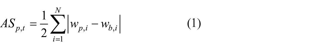
where $w_{p,i}$ and $w_{b,i}$ are the portfolio weights of asset i in mutual fund p and benchmark b. ⁴

We also compute the traditional TE measure of fund activeness to be used as a control variable in our analysis of AS WD. The TE measure is commonly defined as the time-series standard deviation of the difference between a fund return $(R_{p,t})$ and its benchmark return $(R_{b,t})$ . The TE of a given mutual fund p in a given month t is calculated as follows

$$T{E}_{p,t}=Stdev\left[R_{p,t}-R_{b,t}\right]$$

(2)

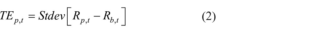
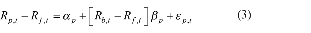
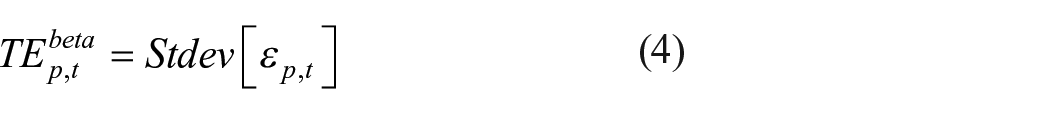
The TE at the end of a given calendar month was calculated using the time series of the previous 120 daily returns. It was later annualized. As expected, the AS and TE measures were positively correlated (.5046). Alternatively, we also calculate the TE by regressing the excess fund returns over the risk-free rate on excess benchmark returns, as follows ⁵

$$R_{p,t}-R_{f,t}={\alpha }_p+\left[R_{b,t}-R_{f,t}\right]{\beta }_p+{\epsilon }_{p,t}$$

(3)

$$T{E}_{p,t}^{beta}=Stdev\left[{\epsilon }_{p,t}\right]$$

(4)

To compute the AS of mutual funds, we require data on the portfolio composition of mutual funds, as well as their benchmarks. The mutual fund holdings database used in this study comprises the monthly portfolio reports of all actively managed Spanish domestic equity funds. This information differs from the previous literature that analyzes quarterly holdings, which implies the loss of interim trades; therefore, it is impossible to test a change in the fund activity level in these interim months. The regulator of the Spanish market, the Spanish Securities and Exchange Commission (CNMV), supplied us with this monthly database until December 2006, after which the information is provided on a quarterly basis (calendar quarter-ends). ⁶ The database is free of survivorship bias because it also includes dead funds. In addition, the database overcomes any possible problem of reporting selection bias that may be present in the scarce research using high-frequency portfolio information, where mutual funds voluntarily supply their portfolio holdings to private data providers (see, for example, Elton et al., 2010).

Our main objective is to test the possible existence of WD at the level of AS shown by equity mutual funds on publicly reported dates (quarter-end months). We therefore focus our study on the time period in which the portfolio holdings of all mutual funds are reported on a monthly basis (1999–2006). ⁷

The initial sample included 169 Spanish domestic equity mutual funds. From this sample, we eliminate passive management funds, such as index funds or exchange traded fund (ETFs), and a couple of funds oriented to Small or Mid-Caps. We begin our analysis in December 2000 because of the requirement of data intended to estimate the momentum factor. The final sample comprises 137 funds from December 2000 to December 2006.

The CNMV mutual fund database provides information on the portfolio holdings and investment vocations of Spanish mutual funds. It also contains other characteristics of mutual funds such as daily and monthly returns, total net assets (TNA), number of investors, annual management fees, fund age, and management company.

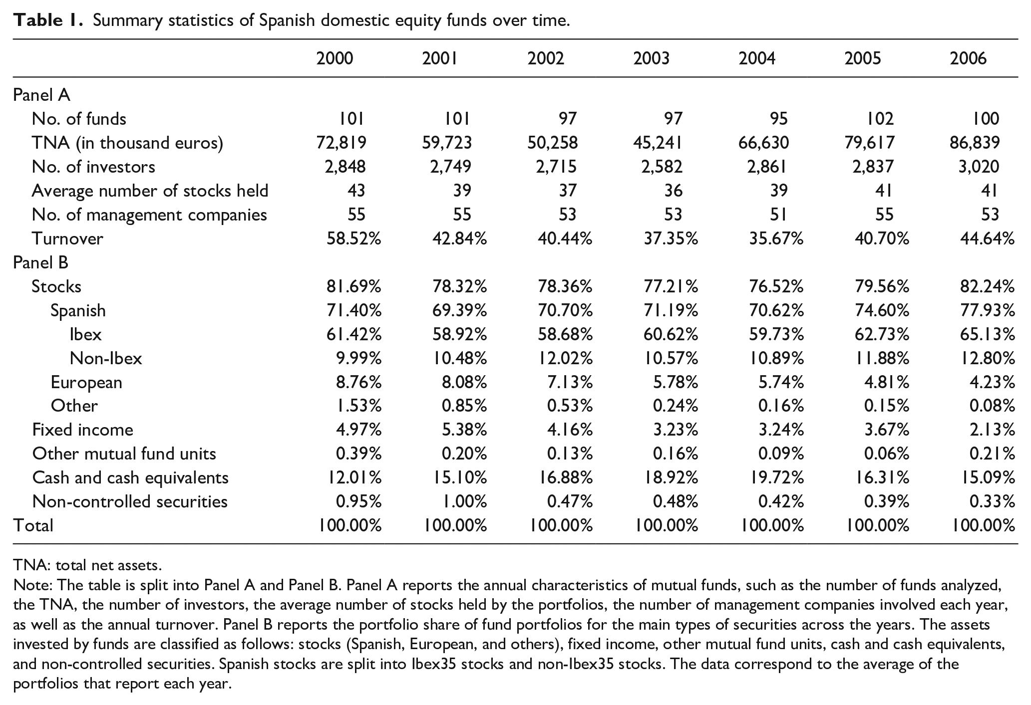
Panel A of Table 1 reports the number of funds examined annually, the average TNA of the funds, the average number of investors, the average number of stocks held by mutual funds, the average number of management companies examined, and the average annual turnover ratio. Specifically, the average TNA of the funds in our sample is €68 million, and the average number of investors is approximately 2,800. Furthermore, the average number of securities held by a fund is 40.

Table 1.

Summary statistics of Spanish domestic equity funds over time.

	2000	2001	2002	2003	2004	2005	2006
Panel A
No. of funds	101	101	97	97	95	102	100
TNA (in thousand euros)	72,819	59,723	50,258	45,241	66,630	79,617	86,839
No. of investors	2,848	2,749	2,715	2,582	2,861	2,837	3,020
Average number of stocks held	43	39	37	36	39	41	41
No. of management companies	55	55	53	53	51	55	53
Turnover	58.52%	42.84%	40.44%	37.35%	35.67%	40.70%	44.64%
Panel B
Stocks	81.69%	78.32%	78.36%	77.21%	76.52%	79.56%	82.24%
Spanish	71.40%	69.39%	70.70%	71.19%	70.62%	74.60%	77.93%
Ibex	61.42%	58.92%	58.68%	60.62%	59.73%	62.73%	65.13%
Non-Ibex	9.99%	10.48%	12.02%	10.57%	10.89%	11.88%	12.80%
European	8.76%	8.08%	7.13%	5.78%	5.74%	4.81%	4.23%
Other	1.53%	0.85%	0.53%	0.24%	0.16%	0.15%	0.08%
Fixed income	4.97%	5.38%	4.16%	3.23%	3.24%	3.67%	2.13%
Other mutual fund units	0.39%	0.20%	0.13%	0.16%	0.09%	0.06%	0.21%
Cash and cash equivalents	12.01%	15.10%	16.88%	18.92%	19.72%	16.31%	15.09%
Non-controlled securities	0.95%	1.00%	0.47%	0.48%	0.42%	0.39%	0.33%
Total	100.00%	100.00%	100.00%	100.00%	100.00%	100.00%	100.00%

TNA: total net assets.

Note: The table is split into Panel A and Panel B. Panel A reports the annual characteristics of mutual funds, such as the number of funds analyzed, the TNA, the number of investors, the average number of stocks held by the portfolios, the number of management companies involved each year, as well as the annual turnover. Panel B reports the portfolio share of fund portfolios for the main types of securities across the years. The assets invested by funds are classified as follows: stocks (Spanish, European, and others), fixed income, other mutual fund units, cash and cash equivalents, and non-controlled securities. Spanish stocks are split into Ibex35 stocks and non-Ibex35 stocks. The data correspond to the average of the portfolios that report each year.

Panel B of Table 1 reports the share of fund portfolios in the main types of securities (stocks, fixed-income securities, other mutual fund units, and cash and cash equivalents) across the years studied. As expected, according to the investment vocation of the funds examined, the main investment is in domestic stocks and, more precisely, in domestic stocks belonging to the Ibex35 index. This panel also shows that the percentage invested in fixed income and other mutual fund units is relatively small. In conclusion, the low percentage of non-controlled securities (less than 1% of the portfolios) reinforces the quality of our database.

We include the Ibex35 index as a benchmark for all funds because it is the most important large-cap index for the Spanish stock market and is, therefore, the most popular self-reported benchmark for our sample of Spanish domestic equity funds (these funds invest, on average, more than 61% of the portfolio in Ibex35 stocks, as shown in Table 1). For all funds, we used the most relevant benchmark for Spanish large-cap equity instead of using the benchmark self-reported by the manager in the fund prospectus because managers can report a misleading benchmark that is easily beaten (Sensoy, 2009). For robustness, we also conducted two analyses: (1) considering the index that produced the lowest AS between Ibex35 index and IGBM (Índice General de Bolsa de Madrid), as in Petajisto (2013) and Cremers and Petajisto (2009), and (2) limiting the analysis to funds that self-reported Ibex35 or IGBM as the benchmark. ⁸

We have historical month-end constituents for the Ibex35 index and IGBM index, and the daily and monthly returns of their constituents from DataStream. This historical information allows us to consider new benchmark constituents and deletions from the benchmarks. All stock holdings, for both mutual funds and benchmarks, were matched with the stock returns through the international securities identification numbering system (ISIN) code for each security.

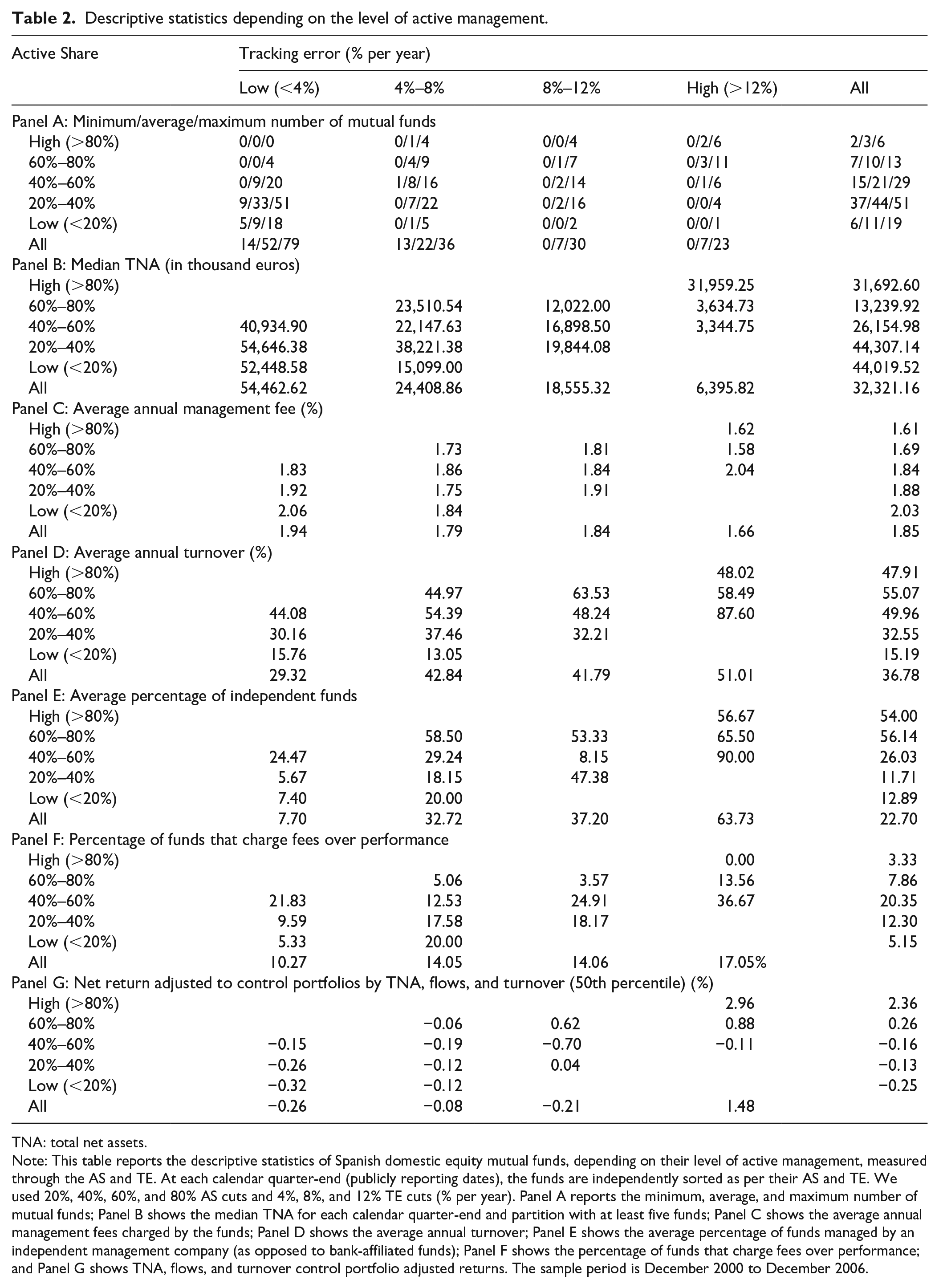
Table 2 shows some descriptive statistics on the distribution of funds along the two dimensions of active management (AS and TE). At each calendar quarter-end (publicly reporting dates), the funds are independently sorted by their AS and TE. We used 20%, 40%, 60%, and 80% AS cuts and 4%, 8%, and 12% TE cuts (% per year). Panel A reports the minimum, average, and maximum number of funds in this bivariate distribution for the sample period and in the univariate marginal distributions along the AS and TE dimensions.

Table 2.

Descriptive statistics depending on the level of active management.

Active Share	Tracking error (% per year)
	Low (<4%)	4%–8%	8%–12%	High (>12%)	All
Panel A: Minimum/average/maximum number of mutual funds
High (>80%)	0/0/0	0/1/4	0/0/4	0/2/6	2/3/6
60%–80%	0/0/4	0/4/9	0/1/7	0/3/11	7/10/13
40%–60%	0/9/20	1/8/16	0/2/14	0/1/6	15/21/29
20%–40%	9/33/51	0/7/22	0/2/16	0/0/4	37/44/51
Low (<20%)	5/9/18	0/1/5	0/0/2	0/0/1	6/11/19
All	14/52/79	13/22/36	0/7/30	0/7/23
Panel B: Median TNA (in thousand euros)
High (>80%)				31,959.25	31,692.60
60%–80%		23,510.54	12,022.00	3,634.73	13,239.92
40%–60%	40,934.90	22,147.63	16,898.50	3,344.75	26,154.98
20%–40%	54,646.38	38,221.38	19,844.08		44,307.14
Low (<20%)	52,448.58	15,099.00			44,019.52
All	54,462.62	24,408.86	18,555.32	6,395.82	32,321.16
Panel C: Average annual management fee (%)
High (>80%)				1.62	1.61
60%–80%		1.73	1.81	1.58	1.69
40%–60%	1.83	1.86	1.84	2.04	1.84
20%–40%	1.92	1.75	1.91		1.88
Low (<20%)	2.06	1.84			2.03
All	1.94	1.79	1.84	1.66	1.85
Panel D: Average annual turnover (%)
High (>80%)				48.02	47.91
60%–80%		44.97	63.53	58.49	55.07
40%–60%	44.08	54.39	48.24	87.60	49.96
20%–40%	30.16	37.46	32.21		32.55
Low (<20%)	15.76	13.05			15.19
All	29.32	42.84	41.79	51.01	36.78
Panel E: Average percentage of independent funds
High (>80%)				56.67	54.00
60%–80%		58.50	53.33	65.50	56.14
40%–60%	24.47	29.24	8.15	90.00	26.03
20%–40%	5.67	18.15	47.38		11.71
Low (<20%)	7.40	20.00			12.89
All	7.70	32.72	37.20	63.73	22.70
Panel F: Percentage of funds that charge fees over performance
High (>80%)				0.00	3.33
60%–80%		5.06	3.57	13.56	7.86
40%–60%	21.83	12.53	24.91	36.67	20.35
20%–40%	9.59	17.58	18.17		12.30
Low (<20%)	5.33	20.00			5.15
All	10.27	14.05	14.06	17.05%
Panel G: Net return adjusted to control portfolios by TNA, flows, and turnover (50th percentile) (%)
High (>80%)				2.96	2.36
60%–80%		−0.06	0.62	0.88	0.26
40%–60%	−0.15	−0.19	−0.70	−0.11	−0.16
20%–40%	−0.26	−0.12	0.04		−0.13
Low (<20%)	−0.32	−0.12			−0.25
All	−0.26	−0.08	−0.21	1.48

TNA: total net assets.

Note: This table reports the descriptive statistics of Spanish domestic equity mutual funds, depending on their level of active management, measured through the AS and TE. At each calendar quarter-end (publicly reporting dates), the funds are independently sorted as per their AS and TE. We used 20%, 40%, 60%, and 80% AS cuts and 4%, 8%, and 12% TE cuts (% per year). Panel A reports the minimum, average, and maximum number of mutual funds; Panel B shows the median TNA for each calendar quarter-end and partition with at least five funds; Panel C shows the average annual management fees charged by the funds; Panel D shows the average annual turnover; Panel E shows the average percentage of funds managed by an independent management company (as opposed to bank-affiliated funds); Panel F shows the percentage of funds that charge fees over performance; and Panel G shows TNA, flows, and turnover control portfolio adjusted returns. The sample period is December 2000 to December 2006.

The Spanish univariate AS distribution differs slightly from that observed in US equity funds. Most of the Spanish domestic equity funds (85% of the funds on average) have an AS lower than 60%, which is the opposite of the distribution observed in the US market. For example, in 2002, only 457 of 1,678 funds (27%) had AS levels lower than 60% in the United States (Table 1, Cremers & Petajisto, 2009) and 82% in Spain. Therefore, the majority of domestic equity funds in Spain fall in the category that Cremers and Petajisto (2009) refer to as closet indexers, that is, funds with low AS levels that claim to be active.

Regarding the percentage of assets under management, the figures from the US and Spanish markets also differ significantly. For example, in December 2006, in the United States, less than 40% of total assets were managed by funds with AS levels lower than 60% (Figure 5, Petajisto, 2013); these accounted for 81% in the Spanish market. Similarly, European Securities and Markets Authority (ESMA, 2016) analyzes the Undertakings for the Collective Investment in Transferable Securities (UCITS) equity funds domiciled in European Union (EU) member states for the period from 2005 to 2012 and finds that 15% of funds have AS levels less than 60% and TE levels less than 4%. However, this type of fund represented 43% of the Spanish sample for the same period. ⁹ ESMA (2016) also measures the percentage of funds with an AS level of less than 50% and a TE level of less than 3%, as these cuts could be more indicative in member states with relatively small equity markets. This report finds that only 7% of funds fall into this category. However, these funds represent 32% of the funds in our sample.

The high fraction of closet indexers in the Spanish mutual fund market can be explained by the smaller size of the Spanish Stock Exchange in comparison to other exchanges, such as those in the United States. The average low level of activeness in the Spanish mutual fund industry can also be explained by the low levels of competitiveness. According to Cremers et al. (2016), markets with less explicit indexing funds are less competitive, and active funds have lower AS levels. Therefore, the low supply of explicit indexing funds in Spain (only 9% of TNA as of December 2010 as stated by Cremers et al., 2016) is another characteristic of the Spanish industry.

The bivariate distribution of funds shows the expected positive relationship between the two active management dimensions. The number of funds with low AS and high TE and vice versa is very low. Nevertheless, as in Cremers and Petajisto (2009), both variables show substantial dispersion in the other dimension. Therefore, both active management measures could have additional explanatory power in terms of fund performance. This finding confirms that it is important to distinguish between the two dimensions of active management.

Panel B of Table 2 reports the median TNA of funds in the AS–TE bivariate distribution. The size of mutual funds tends to decrease monotonically when shifting from the less active to the most active funds. However, this tendency disappears for funds with extreme AS values (more than 80%). This relatively large size of Spanish mutual funds with AS values higher than 80% explains why the percentage of Spanish closet indexers is less extreme when assets under management are considered instead of the number of funds. However, mutual funds with low TE values are the largest group represented in the sample, as in Cremers and Petajisto (2009).

Panel C of Table 2 reports the average annual management and custodial fees charged by Spanish equity mutual funds depending on the bivariate distribution. Contrary to what one could expect, Panel C shows that Spanish domestic equity funds with the lowest AS values charge higher annual management and custodial fees than the remaining funds. This puzzling fact is somehow similar to that found in Gil-Bazo and Ruiz-Verdú (2009), where funds with poor before-fee performance charge higher fees. This finding can be explained by the presence of investors with different levels of sophistication and degrees of sensitivity to past performance. Therefore, we can conclude that the Spanish fund industry is characterized by closet indexers that charge high management fees providing only index-like returns.

Panel D reports an average portfolio turnover of 37% per year, which is lower than the 95% reported by Cremers and Petajisto (2009). The funds with low levels of AS and TE are those with less turnover (lower than 20%). However, we do not find the expected positive relation along the entire distribution.

Panel E shows the average percentage of funds managed by independent management companies. This percentage of funds managed by independent management companies increases with the AS and TE levels. This finding is related to the work of Golez and Marin (2015), who find that Spanish bank-affiliated mutual funds systematically increase their holdings in the controlling bank stock during certain events, such as price drops, indicating that management company ownership matters.

Díaz-Mendoza et al. (2014) found that performance-based fee funds perform significantly better than the other risky funds considered in the Spanish mutual fund industry. Panel F shows the percentage of funds that charge fees based on performance. The results do not support a relationship between fund activeness and this variable.

Finally, Panel G compares the performance mean of the more active funds versus the more passive funds controlling for TNA, flows, and turnover via “control portfolios.” Specifically, net returns are adjusted considering the excess fund net return in a given month in comparison with the “expected” net return according to its TNA, flows, and turnover. Each month, we construct two categories for each of the three above-mentioned variables using the 50th percentile to obtain a sufficient number of portfolios in each of the eight categories. We compute the equally weighted average net returns for each category. We then match each mutual fund month with the TNA–flow–turnover category to which the fund belongs in that month and calculate its adjusted net return as the difference in their net returns. We find that the adjusted returns of control portfolios are positively related to both measures of activeness (AS and TE) and that the funds with the highest levels of AS and TE have the best performance.

To compute the money flows of mutual funds, we follow the absolute and relative money flow measures proposed in previous literature (see, for example, Guercio & Tkac, 2002; Sirri & Tufano, 1998)

$$AbsoluteFlo{w}_{i,t}=TN{A}_{i,t}-TN{A}_{i,t-1}\cdot \left(1+R_{it}\right)$$

(5)

$$RelativeFlo{w}_{i,t}=\frac{TN{A}_{i,t}-TN{A}_{i,t-1}\cdot \left(1+R_{i,t}\right)}{TN{A}_{i,t-1}}$$

(6)

where TNA_i, _t is the total net assets of fund i in month t, and R_i, _t is the return of fund i in month t.

Although the absolute flows are relevant from a management perspective because the vast majority of the funds examined charged their management fees based on TNA, the previous literature has also recommended the use of relative flows when the size of mutual funds is quite dispersed. To avoid potential biases derived from disparities among the average size of the funds according to their level of AS (see Panel B of Table 2), we additionally propose an approach in which money flows are adjusted considering the excess flow attracted by a fund in a given quarter in comparison with the “expected” flow according to its size. Specifically, each month, we construct the TNA deciles and compute their equally weighted average flows. We then match each mutual fund month with the TNA decile in which the fund belongs in that month and calculate its adjusted money flow as the difference in the absolute flows attracted.

Finally, as a proxy to detect AS WD, we compute AS_difference, which is the difference between the AS level in the publicly reported month (end of quarter) and the average AS level in the surrounding non-publicly reported months

$$AS\_differenc{e}_t=A{S}_t-\frac{A{S}_{t-2}+A{S}_{t-1}+A{S}_{t+1}+A{S}_{t+2}}{4}$$

(7)

Empirical models and methods

The influence of active management on future fund performance

Previous studies show that the average mutual fund slightly outperforms the market return before expenses and fails to outperform the market return after expenses (see, for example, Daniel et al., 1997; Fama & French, 2010; Jensen, 1968). Recent studies examining mutual fund trades have demonstrated the superior ability of certain active mutual funds. Chen et al. (2000), Alexander et al. (2007), Baker et al. (2010), and Jiang et al. (2014) find support for the hypothesis of the trading skills of mutual fund managers. ¹⁰

Outperformance can only arise from active management; therefore, there should be cross-sectional differences in fund performance depending on the level of AS. Actively managed funds offer a portfolio that attempts to outperform a reference benchmark by actively deviating from the benchmark weights by overweighting (underweighting) the stocks that the manager considered good (bad) investments. Active mutual funds charge higher fees for active management. Therefore, information regarding the level of active management (AS) is important. It is impossible to beat a benchmark without some level of AS, that is, the lower the level of AS, the lower the possibility of outperforming the benchmark. However, a high level of AS is necessary but is not a sufficient condition to beat the benchmark; this depends on the skill of the manager. Accordingly, Cremers and Petajisto (2009) demonstrate that the AS level in the US market is positively related to fund performance (manager skill).

Given that the incentives to window dress the AS level depend on whether high levels of AS in publicly reported portfolios send a positive signal to potential investors, we first analyze whether the US evidence of the positive effect of AS on subsequent fund performance is observed in the Spanish market (H1). To study the relationship between AS and future fund performance, we run the following pooled panel regression

$$Adj\_Retur{n}_{i,t+1}={\alpha }_0+{\alpha }_{1}A{S}_{i,t}+{\alpha }_{2}T{E}_{i,t}+{\alpha }_{3}Adj\_Retur{n}_{i,t}+control{s}_{i,t}+{\epsilon }_{i,t}$$

(8)

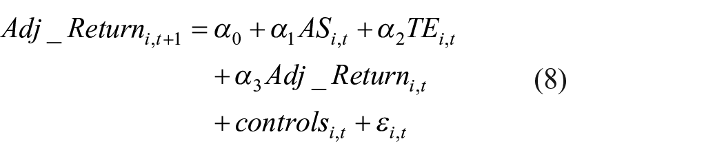
where the dependent variable is the gross or net benchmark adjusted return of mutual funds in month t + 1, while the independent variables are the AS and TE levels of mutual funds, the Adj_Return, and some control variables measured in month t. Specifically, we use the annual turnover, annual management fees, log(TNA), log(TNA)², number of stocks, fund age, number of investors, and annual relative money flows (flows/TNA) as control variables. Year fixed effects are included in all the specifications.

The influence of active management on future money flows

If AS influences future fund performance (H1), we should analyze whether this positive signal given by reporting high levels of AS makes investors more likely to invest in these funds and therefore influences the level of future money flows captured by mutual funds (H2).

To test this hypothesis, we examine the relationship between the AS level and the future money flows received by each mutual fund, including some control variables that could also determine the magnitude of the investment flows, as shown in the following regression

$$Flo{w}_{i,t+1}={\alpha }_0+{\alpha }_{1}A{S}_{i,t}+{\alpha }_{2}T{E}_{i,t}+{\alpha }_{3}Adj\_Retur{n}_{i,t}+control{s}_{i,t}+{\epsilon }_{i,t}$$

(9)

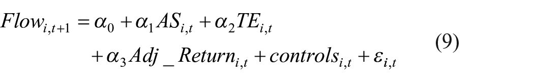
where the dependent variable is the fund money flow in quarter t + 1, defined as the absolute, relative, and adjusted money flows (see equations (5) and (6)). Adjusted money flows are flow deviations from their respective TNA decile flows. The independent variables are the levels of AS and TE of the mutual funds at the end of quarter t, the Adj_Return, and the control variables explained in equation (8). All the explanatory variables are measured at the end of quarter t (publicly disclosed months). Year fixed effects are included in all the specifications. This pooled regression has been conducted on a quarterly basis because the portfolio holdings in the months with no public disclosure are not known to investors. Therefore, they cannot affect future money flows.

Determinants of the AS_difference as proxy to detect AS WD

If the level of activeness measured by AS influences the money flows attracted by Spanish mutual funds, portfolio managers could be tempted to present an artificial image of activeness in publicly disclosed months to achieve more investment flows. To capture potential increments in the AS level reported in publicly disclosed portfolios, we use the AS_difference defined in equation (7). We run the following logit pool regression to analyze the determinants of the AS_difference

$$AS\_diff\_dumm{y}_{i,t}={\alpha }_0+{\alpha }_{1}Adj\_Retur{n}_{i,t-1}+{\alpha }_{2}A{S}_{i,t}+{\alpha }_{3}T{E}_{i,t}+{\alpha }_{4}ReturnGa{p}_{i,t-1}+control{s}_{i,t}+{\epsilon }_{i,t}$$

(10)

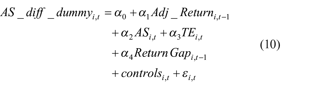
where the dependent variable is a dummy that identifies the AS_difference values between 1% and 2%, 2% and 3%, or those higher than 3% at the end of quarter t. The independent variables are the Adj_Return_i,_t–1 which is the net benchmark adjusted return of mutual funds in the first 2 months of quarter t, the levels of AS and TE, the Return Gap_i,_t–1, ¹¹ and the control variables defined in equation (8), which are all measured at the end of quarter t.

AS WD and future fund performance

In a mutual fund industry where the vast majority of mutual funds charged management fees based on TNA, a relationship between AS level and future money flows could motivate some managers to increase the AS level in publicly reported months, hence making changes in their holding weights with the sole purpose of deviating more from the benchmark weights in the reported month. However, this is not based on the manager’s ability to detect good and bad investments.

Our third hypothesis suggests that because AS WD is not related to the manager’s skill, it will erode fund performance despite the positive relationship between AS and fund performance (H1). Consequently, high levels of positive AS_difference will be negatively related to future fund performance. To test this hypothesis, we run the following pooled panel regression on a quarterly basis

$$Adj\_Retur{n}_{i,t+1}={\alpha }_0+{\alpha }_{1}AS\_diff\_dumm{y}_{i,t}+{\alpha }_{2}A{S}_{i,t}+{\alpha }_{3}T{E}_{i,t}+{\alpha }_{4}Adj\_Retur{n}_{i,t-1}+control{s}_{i,t}+{\epsilon }_{i,t}$$

(11)

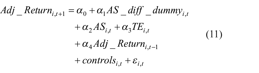
where the dependent variable is the gross or net benchmark adjusted return of mutual funds in quarter t + 1. The independent variables are $AS\_diff\_dumm{y}_{i,t}$ , which is a dummy that identifies AS_difference values higher than 3% at the end of quarter t, the levels of AS and TE at the end of quarter t, the Adj_Return_i,t–1 in the first 2 months of quarter t, and the control variables defined in equation (8), which are all measured at the end of quarter t. Year fixed effects are included in all the specifications. We also run the same regression where the dependent variable is the Carhart (1997) four-factor alphas estimated with daily data of quarter t + 1. ¹²

AS WD and future fund money flows

In this section, we examine whether window-dresser managers reach their objective of attracting higher money flows (H4). To test this hypothesis, we run the following pooled panel regression

$$Flo{w}_{i,t+1}={\alpha }_0+{\alpha }_{1}AS\_diff\_dumm{y}_{i,t}+{\alpha }_{2}A{S}_{i,t}+{\alpha }_{3}T{E}_{i,t}+{\alpha }_{4}Adj\_Retur{n}_{i,t-1}+control{s}_{i,t}+{\epsilon }_{i,t}$$

(12)

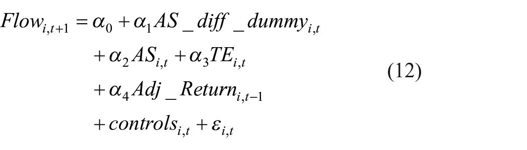
where the dependent variable is the adjusted money flow in quarter t + 1 (flow deviations from their respective TNA decile flow). The independent variables are $AS\_diff\_dumm{y}_{i,t}$ which is a dummy equal to 1 if the AS_difference value is higher than 3% at the end of quarter t, the levels of AS and TE at the end of quarter t, the $Adj\_Retur{n}_{i,t-1}$ in the first 2 months of quarter t, and the control variables defined in equation (8). We include AS as an explanatory variable to control that those funds that window dress attract large flows due to the AS WD disregarding the level of AS itself.

Main results

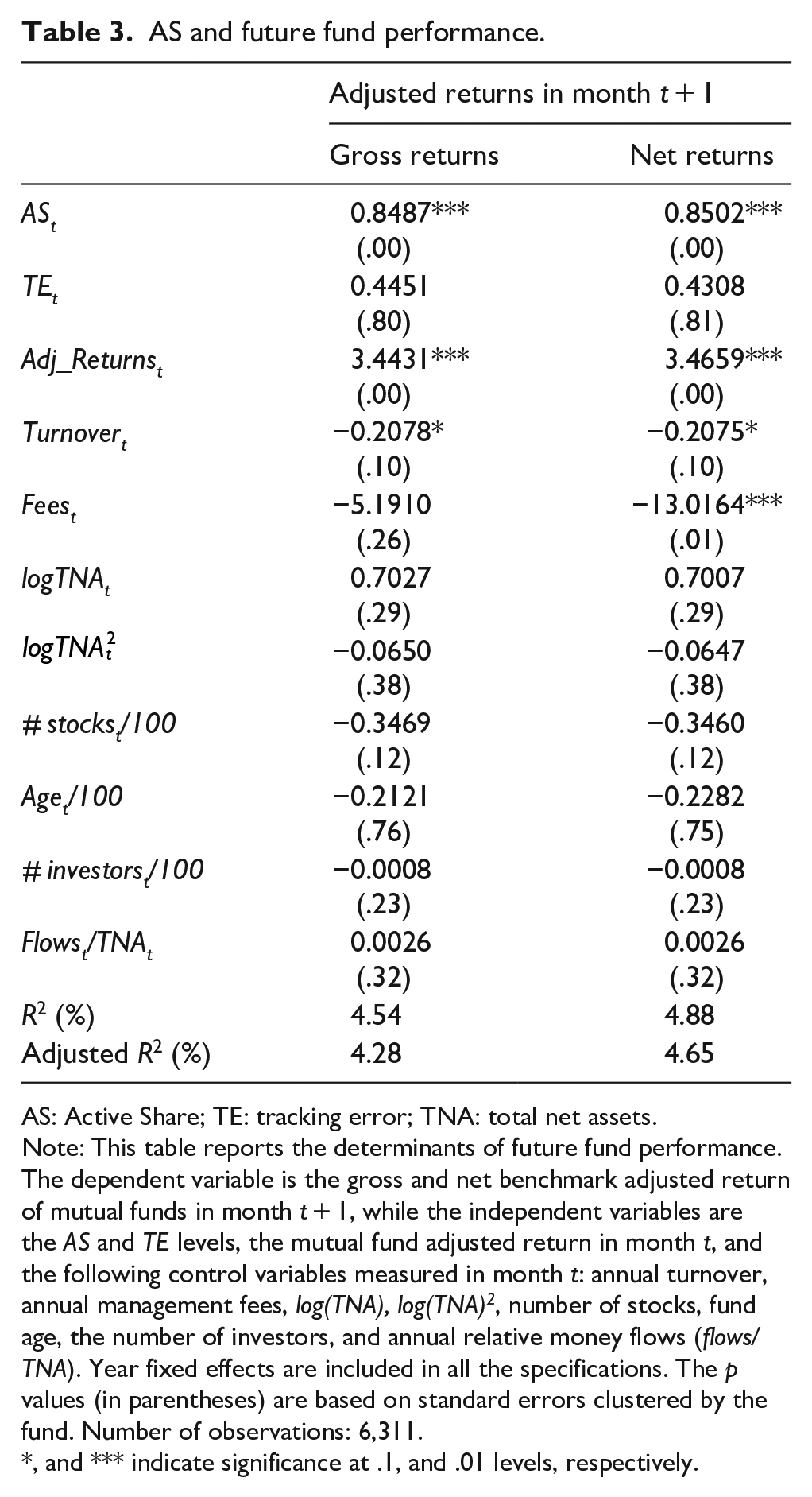
Table 3 shows the results of equation (8) used to test the baseline hypothesis (H1). Our results demonstrate that AS is positively related to future fund returns and, therefore, sends a positive signal about manager skills to beat the benchmark. Moreover, the predictive power of AS on future fund returns is consistent with the inclusion of the traditional active management measure of TE. Therefore, our results are consistent with those of Cremers and Petajisto (2009) in the US market.

Table 3.

AS and future fund performance.

	Adjusted returns in month t + 1
	Gross returns	Net returns
ASt	0.8487*** (.00)	0.8502*** (.00)
TEt	0.4451(.80)	0.4308(.81)
Adj_Returnst	3.4431*** (.00)	3.4659*** (.00)
Turnovert	−0.2078* (.10)	−0.2075* (.10)
Feest	−5.1910(.26)	−13.0164*** (.01)
logTNAt	0.7027(.29)	0.7007(.29)
$logTN{A}_t^2$	−0.0650(.38)	−0.0647(.38)
# stockst/100	−0.3469(.12)	−0.3460(.12)
Aget/100	−0.2121(.76)	−0.2282(.75)
# investorst/100	−0.0008(.23)	−0.0008(.23)
Flowst/TNAt	0.0026(.32)	0.0026(.32)
R2 (%)	4.54	4.88
Adjusted R2 (%)	4.28	4.65

AS: Active Share; TE: tracking error; TNA: total net assets.

Note: This table reports the determinants of future fund performance. The dependent variable is the gross and net benchmark adjusted return of mutual funds in month t + 1, while the independent variables are the AS and TE levels, the mutual fund adjusted return in month t, and the following control variables measured in month t: annual turnover, annual management fees, log(TNA), log(TNA)², number of stocks, fund age, the number of investors, and annual relative money flows (flows/TNA). Year fixed effects are included in all the specifications. The p values (in parentheses) are based on standard errors clustered by the fund. Number of observations: 6,311.

*

, and *** indicate significance at .1, and .01 levels, respectively.

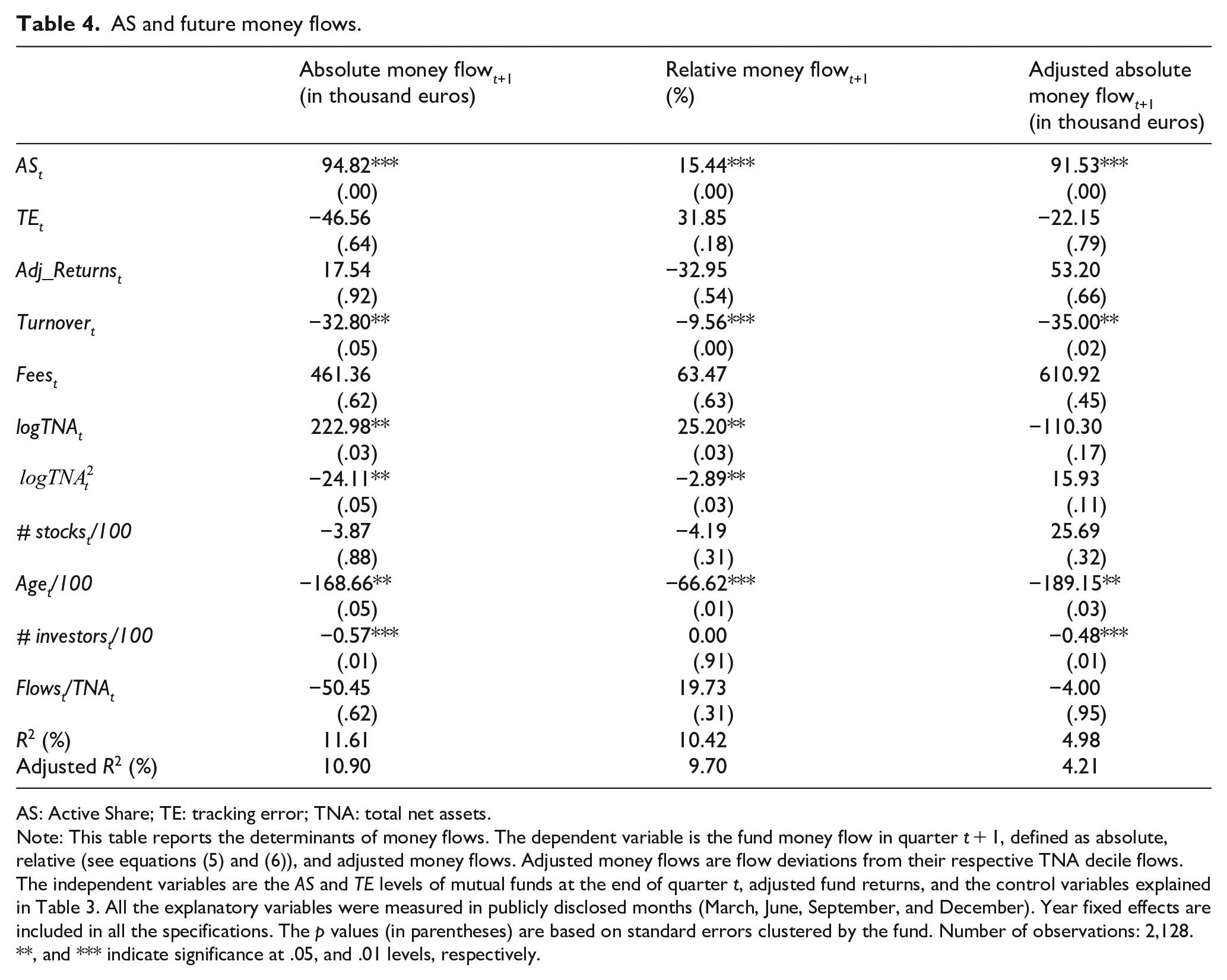
Table 4 shows the results of equation (9) used to test our second hypothesis (H2). The main finding in Table 4 is that the money flows received by mutual funds in a given quarter depend positively on the level of AS previously reported by the fund. The AS variable is positive and statistically significant regardless of whether the absolute, relative, or adjusted money flows are examined. This evidence supports H2. It is also important to note that TE is not statistically significant in any regression. This finding suggests that this dimension of active management does not influence investment flows if AS is included as an explanatory variable. ¹³ Table 4 also shows that relative flows do not effectively control for fund size differences because the variables logTNA and logTNA² have significant coefficients on future flows. The size effect is only appropriately captured when adjusted flows are examined given the lack of significance of logTNA and logTNA² coefficients.

Table 4.

AS and future money flows.

	Absolute money flowt+1 (in thousand euros)	Relative money flowt+1 (%)	Adjusted absolute money flowt+1 (in thousand euros)
ASt	94.82*** (.00)	15.44*** (.00)	91.53*** (.00)
TEt	−46.56(.64)	31.85(.18)	−22.15(.79)
Adj_Returnst	17.54(.92)	−32.95(.54)	53.20(.66)
Turnovert	−32.80** (.05)	−9.56*** (.00)	−35.00** (.02)
Feest	461.36(.62)	63.47(.63)	610.92(.45)
logTNAt	222.98** (.03)	25.20** (.03)	−110.30(.17)
$logTN{A}_t^2$	−24.11** (.05)	−2.89** (.03)	15.93(.11)
# stockst/100	−3.87(.88)	−4.19(.31)	25.69(.32)
Aget/100	−168.66** (.05)	−66.62*** (.01)	−189.15** (.03)
# investorst/100	−0.57*** (.01)	0.00(.91)	−0.48*** (.01)
Flowst/TNAt	−50.45(.62)	19.73(.31)	−4.00(.95)
R2 (%)	11.61	10.42	4.98
Adjusted R2 (%)	10.90	9.70	4.21

AS: Active Share; TE: tracking error; TNA: total net assets.

Note: This table reports the determinants of money flows. The dependent variable is the fund money flow in quarter t + 1, defined as absolute, relative (see equations (5) and (6)), and adjusted money flows. Adjusted money flows are flow deviations from their respective TNA decile flows. The independent variables are the AS and TE levels of mutual funds at the end of quarter t, adjusted fund returns, and the control variables explained in Table 3. All the explanatory variables were measured in publicly disclosed months (March, June, September, and December). Year fixed effects are included in all the specifications. The p values (in parentheses) are based on standard errors clustered by the fund. Number of observations: 2,128.

**

, and *** indicate significance at .05, and .01 levels, respectively.

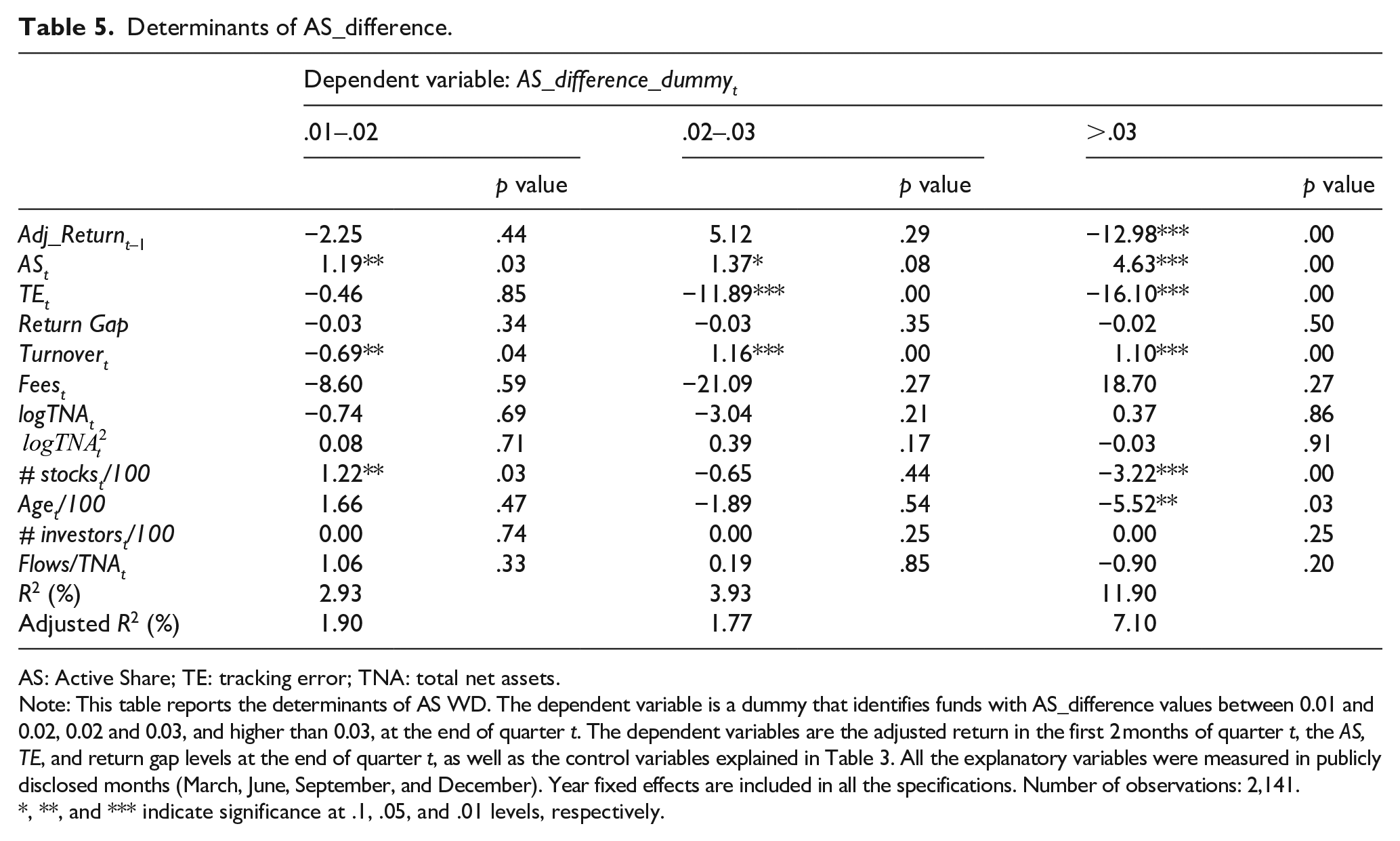
Table 5 shows the determinants of AS_difference values (equation (10)). The most significant results were obtained when the AS_difference_dummy was defined for AS_difference values higher than 3%. High levels of AS_difference are negatively related to fund performance in the previous 2 months. This evidence is consistent with Agarwal et al. (2014), who suggest that the funds that have performed poorly choose WD as the last resort. High levels of AS_difference are positively related to the level of AS. They are, however, negatively related to the level of TE, reflecting that AS window dressers can alter AS rather than TE. The results also show that window-dresser funds incur higher turnover ratios because of the movements needed to window dress the AS level. High levels of AS_difference are also negatively related to the number of stocks in the fund portfolio, which suggest that it is easy to modify a fund with a lower number of stocks. Finally, young funds are more prone to performing WD. The results when the AS_difference level was lower than 3% were less significant, or even showed no significance, for most of the explanatory variables. This evidence suggests that AS_difference values higher than 3% identify window-dresser funds.

Table 5.

Determinants of AS_difference.

	Dependent variable: AS_difference_dummyt
	.01–.02		.02–.03		>.03
		p value		p value		p value
Adj_Returnt –1	−2.25	.44	5.12	.29	−12.98***	.00
ASt	1.19**	.03	1.37*	.08	4.63***	.00
TEt	−0.46	.85	−11.89***	.00	−16.10***	.00
Return Gap	−0.03	.34	−0.03	.35	−0.02	.50
Turnovert	−0.69**	.04	1.16***	.00	1.10***	.00
Feest	−8.60	.59	−21.09	.27	18.70	.27
logTNAt	−0.74	.69	−3.04	.21	0.37	.86
$logTN{A}_t^2$	0.08	.71	0.39	.17	−0.03	.91
# stockst/100	1.22**	.03	−0.65	.44	−3.22***	.00
Aget/100	1.66	.47	−1.89	.54	−5.52**	.03
# investorst/100	0.00	.74	0.00	.25	0.00	.25
Flows/TNAt	1.06	.33	0.19	.85	−0.90	.20
R2 (%)	2.93		3.93		11.90
Adjusted R2 (%)	1.90		1.77		7.10

AS: Active Share; TE: tracking error; TNA: total net assets.

Note: This table reports the determinants of AS WD. The dependent variable is a dummy that identifies funds with AS_difference values between 0.01 and 0.02, 0.02 and 0.03, and higher than 0.03, at the end of quarter t. The dependent variables are the adjusted return in the first 2 months of quarter t, the AS, TE, and return gap levels at the end of quarter t, as well as the control variables explained in Table 3. All the explanatory variables were measured in publicly disclosed months (March, June, September, and December). Year fixed effects are included in all the specifications. Number of observations: 2,141.

*

, **, and *** indicate significance at .1, .05, and .01 levels, respectively.

We analyze the amount of money traded by AS window dressers’ funds to provide an economic valuation of the magnitude of AS WD. At the end of each quarter, we compute the product of AS_difference and TNA in this month for all window-dresser funds (AS_difference > 3%). The monthly average is 21.75 million euros per month. This amount is only 0.71% of the overall TNA of all funds. but this figure represents a significant 11.34% of the TNA of window dressers. Therefore, although the economic impact on the overall fund industry could be insignificant, the economic impact of window dressers is relevant.

As Cremers and Petajisto (2009) point out in Note 7, any WD intended to distort the level of AS at quarter-ends involves incurring large trading costs to achieve a small increase in AS. Therefore, AS increments higher than 3% (and their posterior reversion) are economically significant.

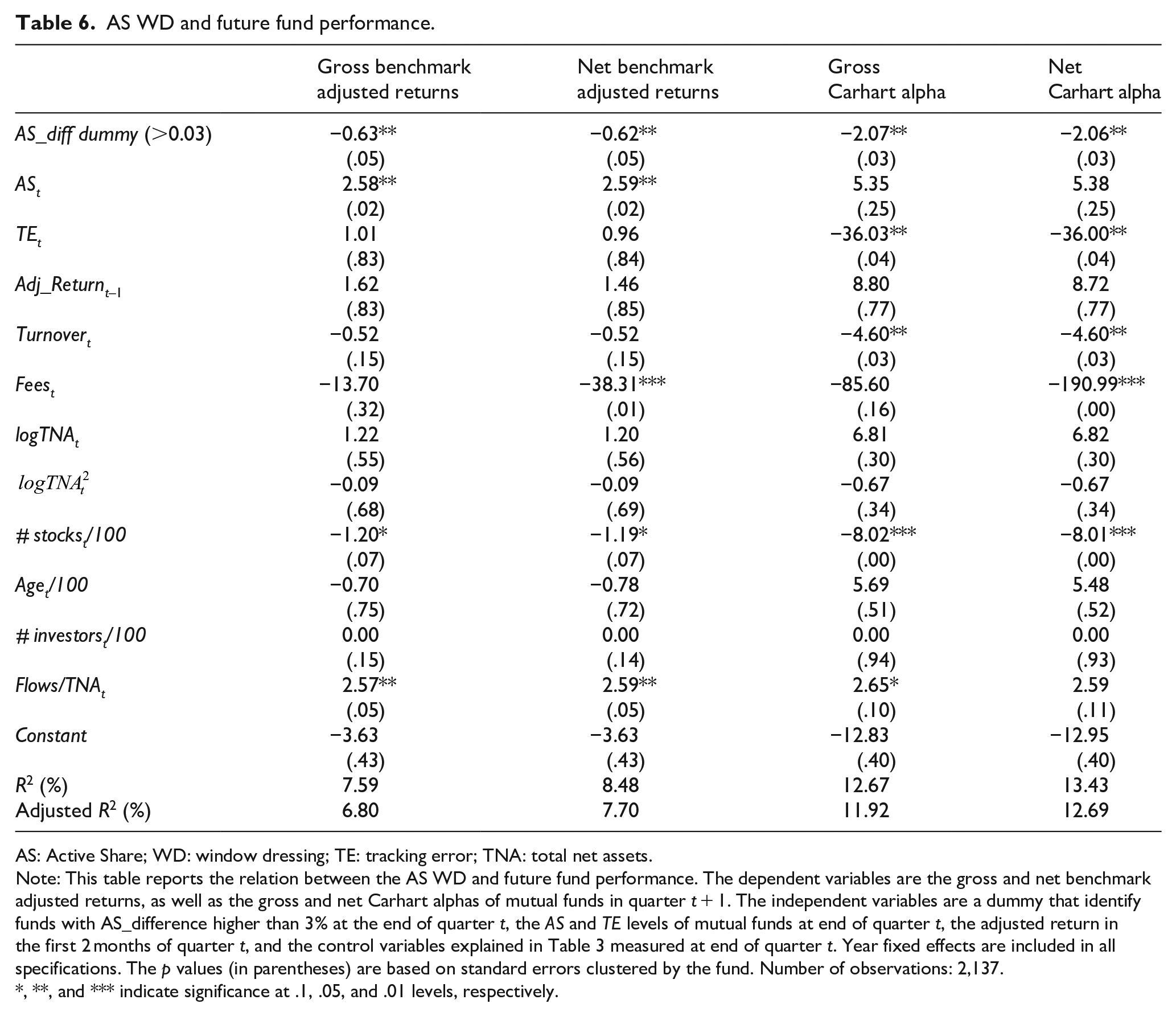
Table 3 shows that future fund returns are positively related to current AS levels. Contrastingly, Table 6 shows that AS_difference values that are higher than 3% negatively influence future fund performance. This evidence supports H3 and the idea that some managers increase AS in publicly reported months; therefore, this trading is not related to the manager’s skill. ¹⁴

Table 6.

AS WD and future fund performance.

	Gross benchmark adjusted returns	Net benchmark adjusted returns	Gross Carhart alpha	Net Carhart alpha
AS_diff dummy (>0.03)	−0.63** (.05)	−0.62** (.05)	−2.07** (.03)	−2.06** (.03)
ASt	2.58** (.02)	2.59** (.02)	5.35(.25)	5.38(.25)
TEt	1.01(.83)	0.96(.84)	−36.03** (.04)	−36.00** (.04)
Adj_Returnt –1	1.62(.83)	1.46(.85)	8.80(.77)	8.72(.77)
Turnovert	−0.52(.15)	−0.52(.15)	−4.60** (.03)	−4.60** (.03)
Feest	−13.70(.32)	−38.31*** (.01)	−85.60(.16)	−190.99*** (.00)
logTNAt	1.22(.55)	1.20(.56)	6.81(.30)	6.82(.30)
$logTN{A}_t^2$	−0.09(.68)	−0.09(.69)	−0.67(.34)	−0.67(.34)
# stockst/100	−1.20* (.07)	−1.19* (.07)	−8.02*** (.00)	−8.01*** (.00)
Aget/100	−0.70(.75)	−0.78(.72)	5.69(.51)	5.48(.52)
# investorst/100	0.00(.15)	0.00(.14)	0.00(.94)	0.00(.93)
Flows/TNAt	2.57** (.05)	2.59** (.05)	2.65* (.10)	2.59(.11)
Constant	−3.63(.43)	−3.63(.43)	−12.83(.40)	−12.95(.40)
R2 (%)	7.59	8.48	12.67	13.43
Adjusted R2 (%)	6.80	7.70	11.92	12.69

AS: Active Share; WD: window dressing; TE: tracking error; TNA: total net assets.

Note: This table reports the relation between the AS WD and future fund performance. The dependent variables are the gross and net benchmark adjusted returns, as well as the gross and net Carhart alphas of mutual funds in quarter t + 1. The independent variables are a dummy that identify funds with AS_difference higher than 3% at the end of quarter t, the AS and TE levels of mutual funds at end of quarter t, the adjusted return in the first 2 months of quarter t, and the control variables explained in Table 3 measured at end of quarter t. Year fixed effects are included in all specifications. The p values (in parentheses) are based on standard errors clustered by the fund. Number of observations: 2,137.

*

, **, and *** indicate significance at .1, .05, and .01 levels, respectively.

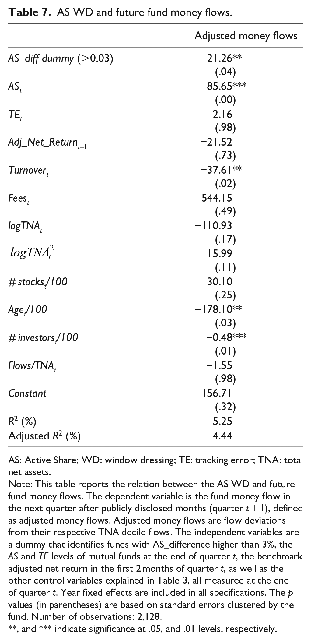
Table 7 reports the results of the relationship between AS WD and future money flows measured as adjusted flows. We observe how funds that increase AS by more than 3% in publicly disclosed months have higher future money flows even after controlling for their AS level. This evidence supports H4.

Table 7.

AS WD and future fund money flows.

	Adjusted money flows
AS_diff dummy (>0.03)	21.26** (.04)
ASt	85.65*** (.00)
TEt	2.16(.98)
Adj_Net_Returnt –1	−21.52(.73)
Turnovert	−37.61** (.02)
Feest	544.15(.49)
logTNAt	−110.93(.17)
$logTN{A}_t^2$	15.99(.11)
# stockst/100	30.10(.25)
Aget/100	−178.10** (.03)
# investorst/100	−0.48*** (.01)
Flows/TNAt	−1.55(.98)
Constant	156.71(.32)
R2 (%)	5.25
Adjusted R2 (%)	4.44

AS: Active Share; WD: window dressing; TE: tracking error; TNA: total net assets.

Note: This table reports the relation between the AS WD and future fund money flows. The dependent variable is the fund money flow in the next quarter after publicly disclosed months (quarter t + 1), defined as adjusted money flows. Adjusted money flows are flow deviations from their respective TNA decile flows. The independent variables are a dummy that identifies funds with AS_difference higher than 3%, the AS and TE levels of mutual funds at the end of quarter t, the benchmark adjusted net return in the first 2 months of quarter t, as well as the other control variables explained in Table 3, all measured at the end of quarter t. Year fixed effects are included in all specifications. The p values (in parentheses) are based on standard errors clustered by the fund. Number of observations: 2,128.

**

, and *** indicate significance at .05, and .01 levels, respectively.

Characteristics of stocks traded by AS window dressers: Is AS WD a practice different from “hot stock” WD?

AS WD and “hot stock” WD are not necessarily the same practice because buying (selling) attractive (unattractive) stocks will increase or decrease the AS level of the fund depending on whether each stock is overweighted or underweighted in the portfolio before the additional trading. However, both practices can be related and the AS WD detected in our study can be a side effect of “hot stock” WD. To rule out this possibility, we run the following regression

$$\begin{array}{l}\%Tradin{g}_{p,i,t}={\alpha }_0+{\alpha }_{1}Adj\_Retur{n}_{i,t-1}+{\alpha }_{2}Adj\_Retur{n}_{i,t-1}\times AS\_diff\_dumm{y}_{p,t}+\\ {\alpha }_3\Delta Abs\_de{v}_{p,i,t}+{\alpha }_4\Delta Abs\_de{v}_{p,i,t}\times AS\_diff\_dumm{y}_{p,t}+{\alpha }_{5}Bet{a}_{i,t-1}+\\ {\alpha }_{6}Bet{a}_{i,t-1}\times AS\_diff\_dumm{y}_{p,t}+{\alpha }_{7}log\left(Siz{e}_{i,t}\right)+{\alpha }_{8}BT{M}_{\mathrm{i},\mathrm{t}}+{\epsilon }_{i,t}\end{array}$$

(13)

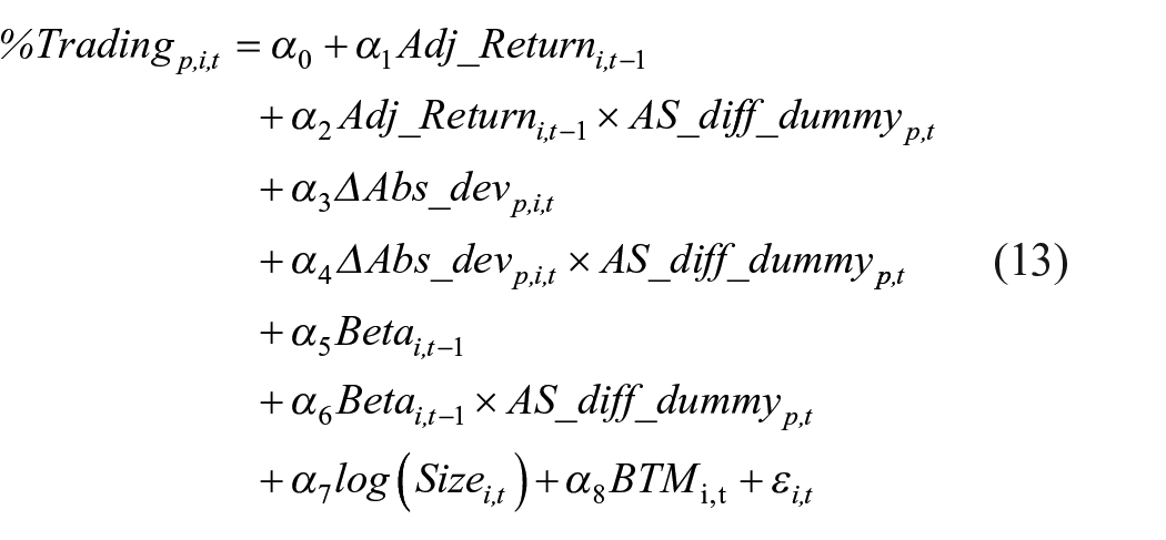
where the dependent variable is the percentage of buying (selling) trading over the TNA of stock i in fund p in the last month of quarter t. The independent variables are the $Adj\_Retur{n}_{i,t-1}$ which is the stock i market adjusted return in the first 2 months of quarter t, $AS\_diff\_dumm{y}_{p,t}$ is a dummy equal to 1 if the AS_difference value is higher than 3% at the end of quarter t, and D $\Delta Abs\_de{v}_{p,i,t}$ measures the absolute deviation of the portfolio weight from the benchmark weight in stock i considering two consecutive periods. $Bet{a}_{i,t-1}$ , $Siz{e}_{i,t-1}$ , and $BT{M}_{i,t-1}$ are the market beta, market capitalization, and book-to-market ratio of stock i in the second month of quarter t.

We compute D $\Delta Abs\_de{v}_{p,i,t}$ as $\left|w_{p,i,t}-w_{b,i,t}\right|-\left|w_{p,i,t-1}-w_{b,i,t-1}\right|$ , where w_p, _i,t and w_b, _i,t are the portfolio weights of asset i in mutual fund p and the benchmark b at the end of quarter t. The positive (negative) values of D $\Delta Abs\_de{v}_{p,i,t}$ show that the stock weight increases (decreases) its deviation from the benchmark. Therefore, stocks with high positive D $\Delta Abs\_de{v}_{p,i,t}$ contribute more to increasing the fund portfolio AS, and stocks with high negative D $\Delta Abs\_de{v}_{p,i,t}$ contribute more to decreasing the fund portfolio AS.

The interaction variable $Adj\_Retur{n}_{i,t-1}\times AS\_diff\_dumm{y}_{p,t}$ measures whether funds that window dress their AS (those with AS_difference > 3%) buy or sell stocks with different past performance to the remaining funds. The interaction variable $\Delta Abs\_de{v}_{p,i,t}\times AS\_diff\_dumm{y}_{p,t}$ measures whether the stocks traded by funds that window dress their AS change their deviation from the benchmark in a different way to that of the remaining funds. To rule out the possibility that AS WD was a side effect of managers taking more risk at quarter-ends, we also include the interaction variable $Bet{a}_{i,t-1}\times AS\_diff\_dumm{y}_{p,t}$ which measures whether those funds that window dress their AS buy or sell stocks with different market beta from the remaining funds.

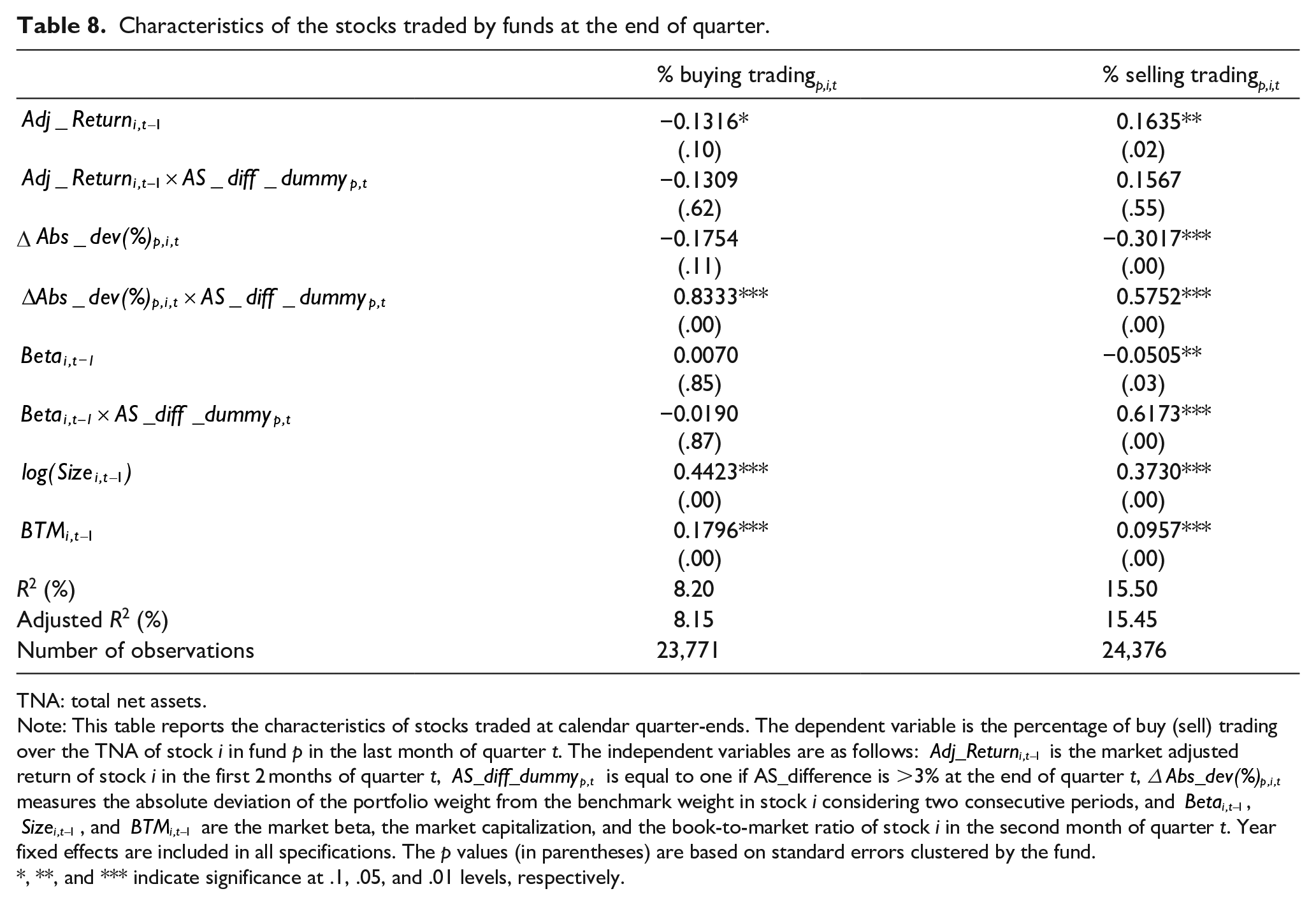
Table 8 presents the results of equation (13). Regarding the past performance of stocks traded at quarter-ends, we first find that funds tend to sell past winners which can be explained by the disposition effect documented in the financial literature. ¹⁵ Second, we find that funds tend to buy past loser stocks which could be interpreted as a search for undervalued stocks. AS window dressers do not show a different behavior (α₂ in equation (13) is not statistically significant), and therefore, they do not tend to buy (sell) past winner (loser) stocks as expected by “hot stocks” WD.

Table 8.

Characteristics of the stocks traded by funds at the end of quarter.

	% buying trading p,i,t	% selling trading p,i,t
$Adj\_Retur{n}_{i,t-1}$	−0.1316* (.10)	0.1635** (.02)
$Adj\_Retur{n}_{i,t-1}\times AS\_diff\_dumm{y}_{p,t}$	−0.1309(.62)	0.1567(.55)
$\Delta Abs\_dev{(\%)}_{p,i,t}$	−0.1754(.11)	−0.3017*** (.00)
$\Delta Abs\_dev{(\%)}_{p,i,t}\times AS\_diff\_dumm{y}_{p,t}$	0.8333*** (.00)	0.5752*** (.00)
$Bet{a}_{i,t–1}$	0.0070(.85)	−0.0505** (.03)
$Bet{a}_{i,t–1}\times ASdiffdumm{y}_{p,t}$	−0.0190(.87)	0.6173*** (.00)
$\log (Siz{e}_{i,t-1})$	0.4423*** (.00)	0.3730*** (.00)
$BT{M}_{i,t-1}$	0.1796*** (.00)	0.0957*** (.00)
R2 (%)	8.20	15.50
Adjusted R2 (%)	8.15	15.45
Number of observations	23,771	24,376

TNA: total net assets.

Note: This table reports the characteristics of stocks traded at calendar quarter-ends. The dependent variable is the percentage of buy (sell) trading over the TNA of stock i in fund p in the last month of quarter t. The independent variables are as follows: $Adj\_Retur{n}_{i,t-1}$ is the market adjusted return of stock i in the first 2 months of quarter t, $AS\_diff\_dumm{y}_{p,t}$ is equal to one if AS_difference is >3% at the end of quarter t, $\Delta Abs\_dev{(\%)}_{p,i,t}$ measures the absolute deviation of the portfolio weight from the benchmark weight in stock i considering two consecutive periods, and $Bet{a}_{i,t-1}$ , $Siz{e}_{i,t-1}$ , and $BT{M}_{i,t-1}$ are the market beta, the market capitalization, and the book-to-market ratio of stock i in the second month of quarter t. Year fixed effects are included in all specifications. The p values (in parentheses) are based on standard errors clustered by the fund.

*

, **, and *** indicate significance at .1, .05, and .01 levels, respectively.

Regarding weight deviation from the benchmark in publicly disclosed months, we find that, on average, sales tend to reduce weight deviations. Furthermore, purchases do not have a significant impact. However, the most relevant finding is the different behavior shown by the funds that try to appear more active at quarter-ends (α₄ coefficient in equation (13)). These funds tend to increase their weight deviation to the benchmark in reporting dates relative to the remaining funds that tend to decrease the deviation. This evidence corroborates that our variable AS_difference value higher than 3% captures the funds that window dress their AS, and that it is not a side effect of “hot stock” WD.

Finally, the Beta coefficients rule out the possibility that AS WD was a side effect of managers taking more risk at quarter-ends. Stocks purchased by AS window dressers do not show a beta different from the remaining funds. Stocks sold by AS window dressers have a beta significantly higher than the remaining funds; therefore, this behavior reduces, instead of increases, the risk of the fund portfolio.

Examining the funds that are more prone to window dress the AS level

Our study also focuses on detecting funds that are more prone to altering the AS level. The level of deviation from a benchmark can be altered by portfolio managers because its value can increase or decrease as a consequence of trades (as demonstrated in the previous section). However, other measures used to capture the level of activity, such as TE, cannot be distorted because the daily TNA values of the funds are publicly available. The requirement of high or low levels in both measures of activeness (TE and AS) deletes the funds that are probably altering the holdings at quarter-ends. In other words, among high AS funds, some portfolios could alter their holdings to appear more active. However, these would fall into the category of low TE as they cannot alter their TE. Therefore, AS WD would be concentrated in the high AS and low TE portfolio category.

To test this, we divided the mutual funds into four categories according to their levels of AS and TE. At each calendar quarter-end (i.e., March, June, September, and December), funds are independently ranked into two categories of AS and TE using the 80th percentile. Therefore, the high AS fund category gathers 20% of funds with the highest level of AS and the low AS fund category brings together the remaining 80% of funds. The same is done for the TE categories to form four categories from their intersection.

We use independent ranks instead of the conditional ranks used in Cremers and Petajisto (2009) because independent ranks (as used by Fama and French to construct their factors) allow for better orthogonalization. Moreover, in conditional ranks, the results depend on which variable is first used to rank. ¹⁶ As shown in Table 2, independent ranks of positively related variables, such as AS and TE, result in empty categories (low AS and high TE, and vice versa) for most of the formation dates. To avoid empty categories, we used the 80th percentile. During the 25 ranking months, the percentage of funds with AS values higher than 60% ranges from 12% to 20%, so we believe that the 80th percentile is a reasonable break point for separating active funds from closet index funds. ¹⁷

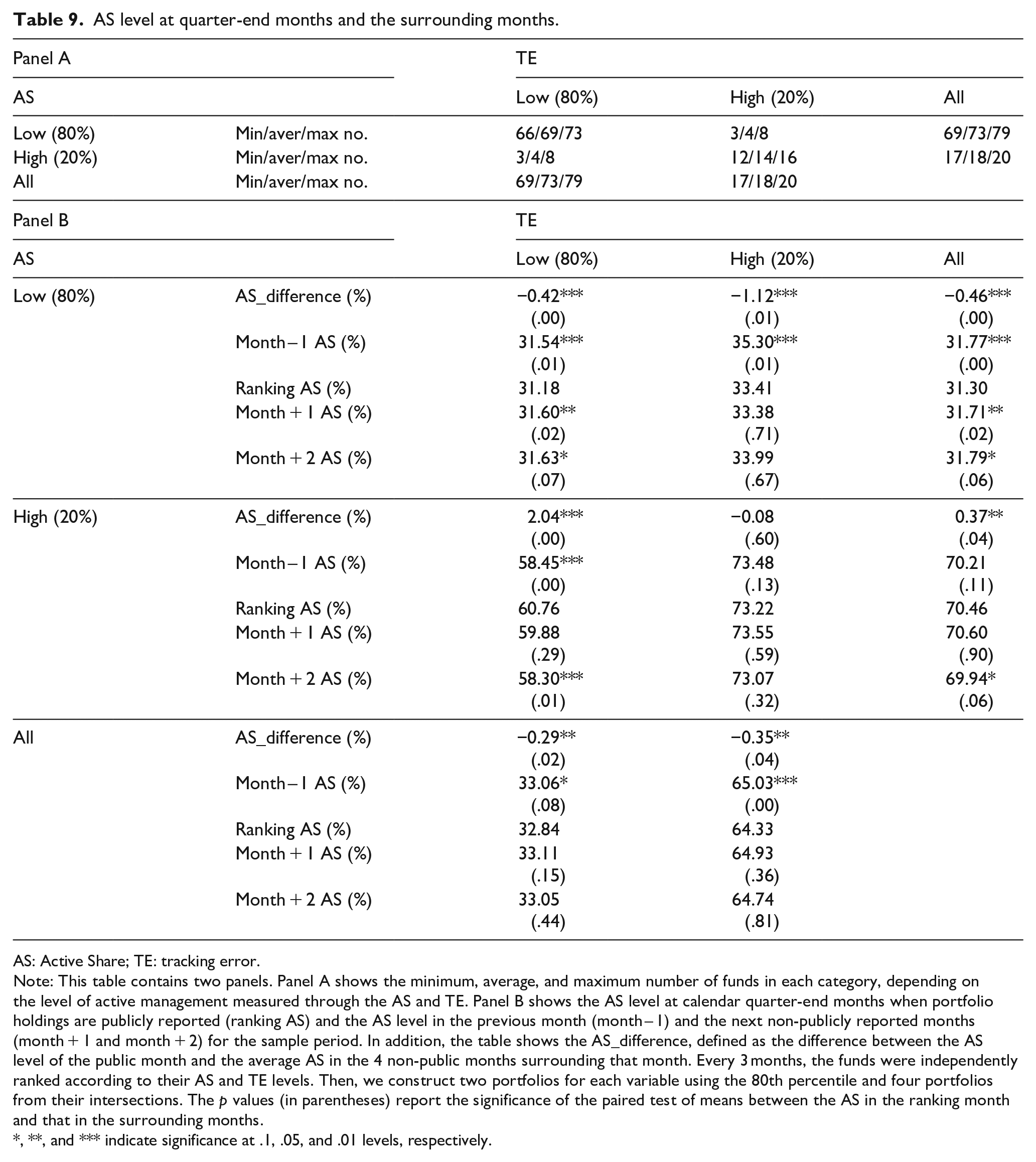
Table 9 shows descriptive statistics of the minimum, average, and maximum number of funds (Panel A) and AS_difference (Panel B) for each of the four AS–TE categories. Consistent with our idea, only the category of funds with high AS and low TE shows a positive and statistically significant value of the AS_difference (2.04%). ¹⁸

Table 9.

AS level at quarter-end months and the surrounding months.

Panel A		TE
AS		Low (80%)	High (20%)	All
Low (80%)	Min/aver/max no.	66/69/73	3/4/8	69/73/79
High (20%)	Min/aver/max no.	3/4/8	12/14/16	17/18/20
All	Min/aver/max no.	69/73/79	17/18/20
Panel B		TE
AS		Low (80%)	High (20%)	All
Low (80%)	AS_difference (%)	−0.42*** (.00)	−1.12*** (.01)	−0.46*** (.00)
	Month – 1 AS (%)	31.54*** (.01)	35.30*** (.01)	31.77*** (.00)
	Ranking AS (%)	31.18	33.41	31.30
	Month + 1 AS (%)	31.60** (.02)	33.38(.71)	31.71** (.02)
	Month + 2 AS (%)	31.63* (.07)	33.99(.67)	31.79* (.06)
High (20%)	AS_difference (%)	2.04*** (.00)	−0.08(.60)	0.37** (.04)
	Month – 1 AS (%)	58.45*** (.00)	73.48(.13)	70.21(.11)
	Ranking AS (%)	60.76	73.22	70.46
	Month + 1 AS (%)	59.88(.29)	73.55(.59)	70.60(.90)
	Month + 2 AS (%)	58.30*** (.01)	73.07(.32)	69.94* (.06)
All	AS_difference (%)	−0.29** (.02)	−0.35** (.04)
	Month – 1 AS (%)	33.06* (.08)	65.03*** (.00)
	Ranking AS (%)	32.84	64.33
	Month + 1 AS (%)	33.11(.15)	64.93(.36)
	Month + 2 AS (%)	33.05(.44)	64.74(.81)

AS: Active Share; TE: tracking error.

Note: This table contains two panels. Panel A shows the minimum, average, and maximum number of funds in each category, depending on the level of active management measured through the AS and TE. Panel B shows the AS level at calendar quarter-end months when portfolio holdings are publicly reported (ranking AS) and the AS level in the previous month (month – 1) and the next non-publicly reported months (month + 1 and month + 2) for the sample period. In addition, the table shows the AS_difference, defined as the difference between the AS level of the public month and the average AS in the 4 non-public months surrounding that month. Every 3 months, the funds were independently ranked according to their AS and TE levels. Then, we construct two portfolios for each variable using the 80th percentile and four portfolios from their intersections. The p values (in parentheses) report the significance of the paired test of means between the AS in the ranking month and that in the surrounding months.

*

, **, and *** indicate significance at .1, .05, and .01 levels, respectively.

Table 9 also analyzes the statistical significance of the difference between the level of AS in the publicly disclosed months in comparison to the level of AS in the previous month (month – 1), as well as the level in the next 2 months (month + 1 and month + 2), in which fund holdings are not officially available for fund competitors and investors. Mutual funds characterized by a high value of AS and a low value of TE show a statistically significant increase in their level of AS in the month in which portfolios are made public. In addition, we observe a decrease in the level of AS from quarter-end months to month + 1 and month + 2. However, the decrease is only statistically significant from quarter-end to month + 2.

Table 9 also shows that low AS funds tend to reduce their AS levels when their holdings are made public. Therefore, it seems that these funds attempt to portray an image that does not deviate excessively from the benchmark. This finding is particularly interesting in mutual funds with low AS and high TE levels, given that the TE level with respect to the benchmark indicates active management.

To further investigate the characteristics of funds more prone to WD, we conduct an additional analysis with a parametric methodology rather than the difference in the AS means calculated in Table 9. We run the following pooled panel regression

$$\Delta A{S}_{i,t}={\alpha }_0+{\alpha }_{1}D\_Publi{c}_{i,t}+control{s}_{i,t}+{\epsilon }_{i,t}$$

(14)

where the dependent variable is the change in AS in month t, α₀ is a constant, and D_Public is a dummy variable that equals 1 for publicly disclosed months (calendar quarter-ends), and 0 otherwise. We run this regression for the two AS categories and for each of the four AS–TE fund categories. Once a fund is ranked in a given category in each calendar quarter-end, it remains in the same category during the following 2 months. The control variables are TE, Adj_Return, and those defined in equation (8).

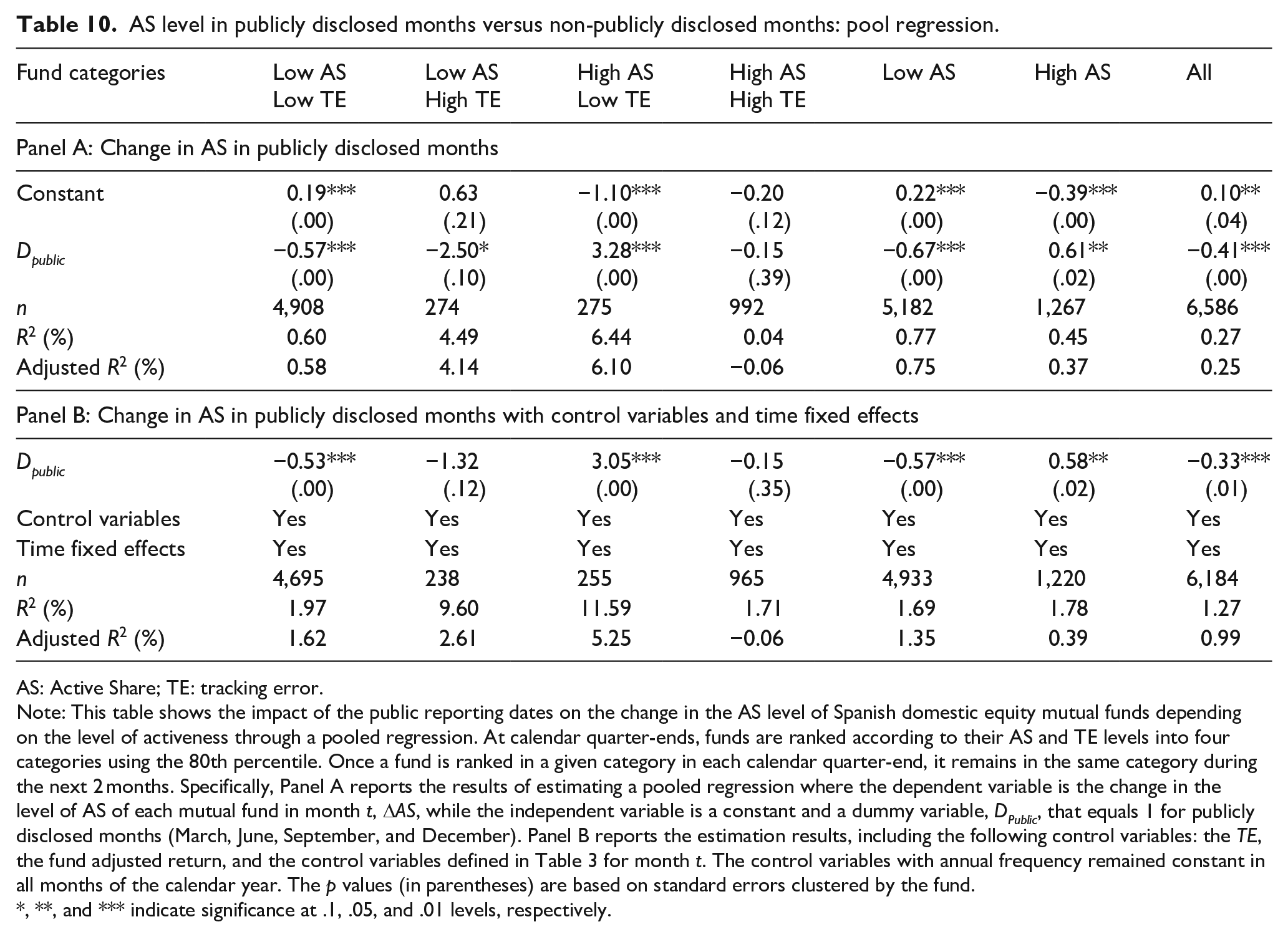
Therefore, the constant coefficient measures the average ∆AS in non-publicly reported months, and the coefficient of the dummy measures how the average ∆AS in publicly reported months deviates from the former. Table 10 shows the results.

Table 10.

AS level in publicly disclosed months versus non-publicly disclosed months: pool regression.

Fund categories	Low ASLow TE	Low ASHigh TE	High ASLow TE	High ASHigh TE	Low AS	High AS	All
Panel A: Change in AS in publicly disclosed months
Constant	0.19*** (.00)	0.63(.21)	−1.10*** (.00)	−0.20(.12)	0.22*** (.00)	−0.39*** (.00)	0.10** (.04)
Dpublic	−0.57*** (.00)	−2.50* (.10)	3.28*** (.00)	−0.15(.39)	−0.67*** (.00)	0.61** (.02)	−0.41*** (.00)
n	4,908	274	275	992	5,182	1,267	6,586
R2 (%)	0.60	4.49	6.44	0.04	0.77	0.45	0.27
Adjusted R2 (%)	0.58	4.14	6.10	−0.06	0.75	0.37	0.25
Panel B: Change in AS in publicly disclosed months with control variables and time fixed effects
Dpublic	−0.53*** (.00)	−1.32(.12)	3.05*** (.00)	−0.15(.35)	−0.57*** (.00)	0.58** (.02)	−0.33*** (.01)
Control variables	Yes	Yes	Yes	Yes	Yes	Yes	Yes
Time fixed effects	Yes	Yes	Yes	Yes	Yes	Yes	Yes
n	4,695	238	255	965	4,933	1,220	6,184
R2 (%)	1.97	9.60	11.59	1.71	1.69	1.78	1.27
Adjusted R2 (%)	1.62	2.61	5.25	−0.06	1.35	0.39	0.99

AS: Active Share; TE: tracking error.

Note: This table shows the impact of the public reporting dates on the change in the AS level of Spanish domestic equity mutual funds depending on the level of activeness through a pooled regression. At calendar quarter-ends, funds are ranked according to their AS and TE levels into four categories using the 80th percentile. Once a fund is ranked in a given category in each calendar quarter-end, it remains in the same category during the next 2 months. Specifically, Panel A reports the results of estimating a pooled regression where the dependent variable is the change in the level of AS of each mutual fund in month t, ∆AS, while the independent variable is a constant and a dummy variable, D_Public, that equals 1 for publicly disclosed months (March, June, September, and December). Panel B reports the estimation results, including the following control variables: the TE, the fund adjusted return, and the control variables defined in Table 3 for month t. The control variables with annual frequency remained constant in all months of the calendar year. The p values (in parentheses) are based on standard errors clustered by the fund.

*

, **, and *** indicate significance at .1, .05, and .01 levels, respectively.

Table 10 shows that, on average, Spanish equity mutual funds tend to reduce the AS level in publicly reported months in relation to the average AS change in non-publicly reported months (a statistically significant −0.41%). This finding is consistent with the evidence provided in Table 8 and with the results provided in Table 9. This result can be partially explained by the fact that most of the funds are classified as low AS and low TE. Furthermore, these funds attempt to appear less active in quarter-ends, probably because they are oriented to conservative investors looking for low active management.

When the different fund categories according to their active management are analyzed, we observe that this tendency to reduce AS in publicly reported months is exclusive to low AS funds. The changes in the AS levels in the high AS and low TE funds are the opposite. These funds tend to increase the AS level in publicly reported months relative to the average AS change in non-publicly reported months (a statistically significant 3.28%). Finally, as expected, funds with both high AS and TE do not exhibit different behavior in their monthly AS changes because this category gathers these mutual funds with real active management captured by both metrics, that is, AS and TE. The results are consistent when the control variables and time fixed effects are included.

In summary, this study provides evidence of a certain type of WD to appear more active conducted by mutual funds with a high level of AS and a low level of TE when portfolios are publicly available to financial market participants.

Robustness analyses

High AS–low TE funds and future performance

In the previous section, we found that funds with high AS but low TE levels exhibit higher levels of AS_difference. In this section, we attempt to provide additional evidence by analyzing the future performance of the four fund categories. If this measure actually measures AS WD, then we should expect the high AS and low TE fund category to exhibit worse performance than the funds with a similar level of AS, but with no distortion, that is, high AS and high TE funds.

Table 11 shows the annualized values of the benchmark adjusted returns (Panel A) and the four-factor alphas (Panel B) in quarter t + 1 for each of the four categories of funds and for both gross and net returns. ¹⁹ Funds with high AS and low TE levels not only exhibit worse performance than funds with high AS and TE, they are the fund category with the worst performance. The funds included in this category fail to reach the expected levels of good performance related to their high level of AS.

Table 11.

Annual performance according to the level of active management.

Panel A		TE
AS		Low (80%)	High (20%)	All	High–low
Low (80%)	Gross adjusted return (%)	−0.76(.15)	−0.29(.92)	−0.76(.21)	0.47(.85)
	Net adjusted return (%)	−2.66*** (.00)	−2.20(.45)	−2.67*** (.00)	0.46(.86)
High (20%)	Gross adjusted return (%)	−3.28** (.05)	5.81(.11)	3.43(.26)	9.08*** (.01)
	Net adjusted return (%)	−5.10*** (.00)	4.16(.26)	1.75(.56)	9.26*** (.01)
				High–low TE	High–low AS
All	Gross adjusted return (%)	−0.93* (.09)	4.24(.22)	5.17* (.10)	4.19* (.10)
	Net adjusted return (%)	−2.83*** (.00)	2.53(.46)	5.37* (.08)	4.41* (.08)
					Mix H-L
High-low	Gross adjusted return (%)	−2.52* (.09)	6.10*** (.00)		6.56** (.05)
	Net adjusted return (%)	−2.44* (.10)	6.36*** (.00)		6.82** (.04)
Panel B		TE
AS		Low (80%)	High (20%)	All	High–low
Low (80%)	Gross alpha 4 (%)	−1.09*** (.00)	−2.67* (.10)	−1.23*** (.00)	−1.57(.30)
	Net alpha 4 (%)	−2.98*** (.00)	−4.57*** (.01)	−3.12*** (.00)	−1.59(.30)
High (20%)	Gross alpha 4 (%)	−4.56** (.02)	1.88(.34)	0.17(.93)	6.44*** (.00)
	Net alpha 4 (%)	−6.38*** (.00)	0.25(.90)	−1.49(.43)	6.63*** (.00)
				High–low TE	High–low AS
All	Gross alpha 4 (%)	−1.30*** (.00)	0.66(.71)	1.96(.24)	1.40(.42)
	Net alpha 4 (%)	−3.19*** (.00)	−1.02(.57)	2.16(.20)	1.63(.35)
					Mix H-L
High-low	Gross alpha 4 (%)	−3.47** (.04)	4.54*** (.00)		2.97(.11)
	Net alpha 4 (%)	−3.40** (.05)	4.82*** (.00)		3.23* (.08)

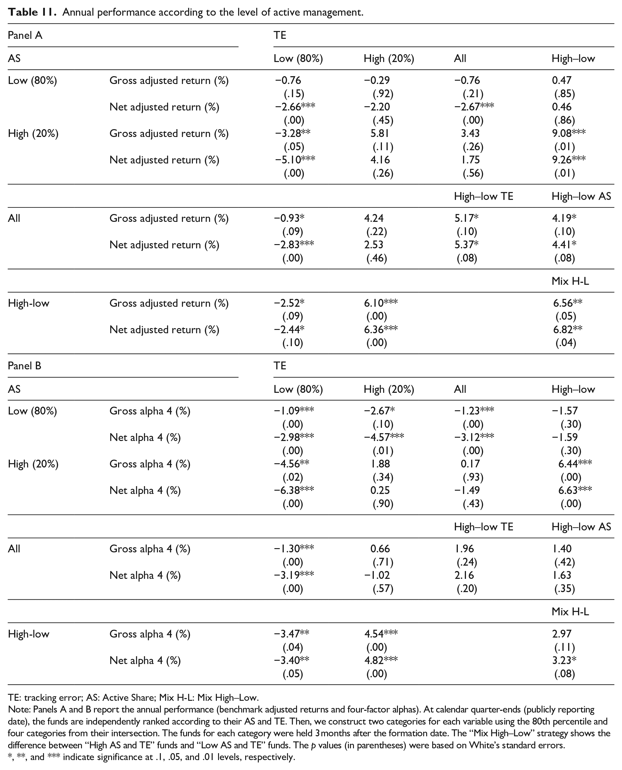
TE: tracking error; AS: Active Share; Mix H-L: Mix High–Low.

Note: Panels A and B report the annual performance (benchmark adjusted returns and four-factor alphas). At calendar quarter-ends (publicly reporting date), the funds are independently ranked according to their AS and TE. Then, we construct two categories for each variable using the 80th percentile and four categories from their intersection. The funds for each category were held 3 months after the formation date. The “Mix High–Low” strategy shows the difference between “High AS and TE” funds and “Low AS and TE” funds. The p values (in parentheses) were based on White’s standard errors.

*

, **, and *** indicate significance at .1, .05, and .01 levels, respectively.

Table 11 also shows other interesting relations that are different from those observed in the US market. First, we found that neither AS nor TE can provide a positive and statistically significant performance. This finding differs from that of Cremers and Petajisto (2009), who show that AS allows investors to select funds with good performance. However, our results are consistent with Cremers et al. (2016), who state that the average alphas generated by active management are lower in markets where closet indexing is generalized. Second, we also find that the AS level predicts fund performance among high TE funds (the difference in the four-factor alpha between high AS and low AS is above 4%, a figure positive and statistically significant for both gross and net). Similarly, the TE level predicts the fund performance among high AS funds (the difference in the four-factor alpha is also above 4%). This last finding differs from that of Cremers and Petajisto (2009), who do not observe that TE predicts fund performance within any AS category. The differences in the findings may be because we independently rank funds according to both metrics to obtain appropriate orthogonal portfolios, while these authors sort funds into AS first and then into TE quintiles. Sorting funds first into AS and then into TE tests whether TE has predictive power after controlling for AS, but not the contrary. To analyze the predictive power of AS controlling for TE, funds should first be sorted into TE. Third, we can perform a better selection if we focus on the funds that simultaneously have high levels of both active measures. Although funds with both high AS and TE levels do not yield significant positive performance, it must be highlighted that, in contrast to the other funds, on average, they are the only category able to generate enough value to, at least, compensate for their fees. ²⁰

High AS–low TE funds and future money flows

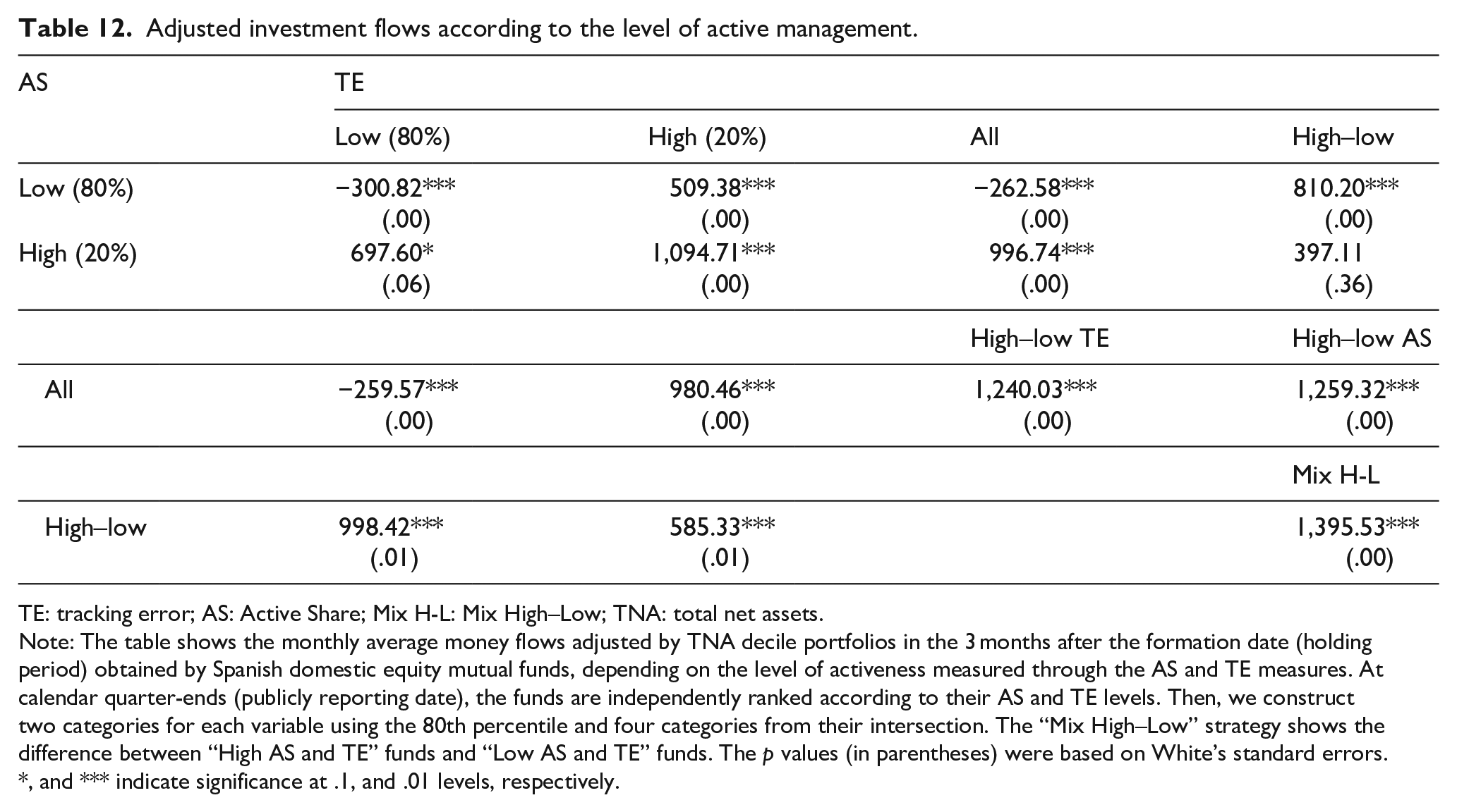
In this section, we attempt to provide extra support to H4 by analyzing the relationship between the different categories of active management based on AS and TE and their money flows. Table 12 shows the monthly average adjusted flow in the 3 months after the formation date (holding period) for each of the four portfolio categories. We find that despite the worst performance of window dressers (high AS–low TE funds), these funds do not exhibit significantly lower levels of money flows than the category of funds with both high AS and TE. Furthermore, they attract significantly higher money flows than funds with both low AS and TE. Therefore, window-dresser funds reach the objective of attracting money flows. This evidence supports H4.

Table 12.

Adjusted investment flows according to the level of active management.

AS	TE
	Low (80%)	High (20%)	All	High–low
Low (80%)	−300.82*** (.00)	509.38*** (.00)	−262.58*** (.00)	810.20*** (.00)
High (20%)	697.60* (.06)	1,094.71*** (.00)	996.74*** (.00)	397.11(.36)
			High–low TE	High–low AS
All	−259.57*** (.00)	980.46*** (.00)	1,240.03*** (.00)	1,259.32*** (.00)
				Mix H-L
High–low	998.42*** (.01)	585.33*** (.01)		1,395.53*** (.00)

TE: tracking error; AS: Active Share; Mix H-L: Mix High–Low; TNA: total net assets.

Note: The table shows the monthly average money flows adjusted by TNA decile portfolios in the 3 months after the formation date (holding period) obtained by Spanish domestic equity mutual funds, depending on the level of activeness measured through the AS and TE measures. At calendar quarter-ends (publicly reporting date), the funds are independently ranked according to their AS and TE levels. Then, we construct two categories for each variable using the 80th percentile and four categories from their intersection. The “Mix High–Low” strategy shows the difference between “High AS and TE” funds and “Low AS and TE” funds. The p values (in parentheses) were based on White’s standard errors.

*

, and *** indicate significance at .1, and .01 levels, respectively.

AS WD and future performance: Monthly basis regression and independent funds subsample

In addition to the quarterly based regression of equation (11), we also analyzed the impact of AS WD in publicly disclosed months on future performance in a monthly basis regression, as shown in the following equation

$$Adj\_Return{s}_{i,t+1}={\alpha }_0+{\alpha }_{1}D\_Publi{c}_{i,t}+{\alpha }_{2}A{S}_{i,t}+{\alpha }_{3}D\_Publi{c}_{i,t}\times A{S}_{i,t}+control{s}_{i,t}+{\epsilon }_{i,t}$$

(15)

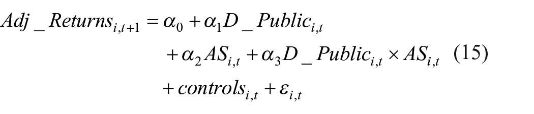
where the dependent variable is the gross and net adjusted returns of mutual funds in the next month t + 1, while the independent variables are as follows: $D\_Public$ is a dummy variable that equals 1 for publicly disclosed months, and 0 otherwise; AS of mutual funds in month t; and the interaction between $D\_Publi{c}_{i,t}$ and $A{S}_{i,t}$ . The control variables are TE, Adj_Returns, and those defined in equation (8).

Hence, the interaction variable, $D\_Publi{c}_{i,t}\times A{S}_{i,t}$ , measures deviations of AS in publicly disclosed months from non-publicly disclosed months and, therefore, could be considered a proxy for changing the holdings to appear more active. If the practice of artificially increasing the level of AS in publicly disclosed months deteriorates fund performance, then we should expect negative coefficients for this variable.

Moreover, we suggest that the negative performance impact of changing portfolio holdings in publicly disclosed months depends on how this practice is conducted. Accordingly, Golez and Marin (2015) find that Spanish bank-affiliated mutual funds (non-independent funds) make holding changes based on the bank’s interest. Based on this previous evidence, we hypothesize that independent funds are, on average, less prone to performing WD, and if they increase the AS level in publicly reported months (high levels of AS_difference), it will more likely be related to informed transactions rather than AS WD. Therefore, they will not damage performance. In contrast, non-independent funds are, on average, more prone to performing WD (subject to the interest of the bank they are affiliated with). If they increase the AS level in publicly reported months, it will probably be related to WD rather than to informed trading. Therefore, they will damage performance.

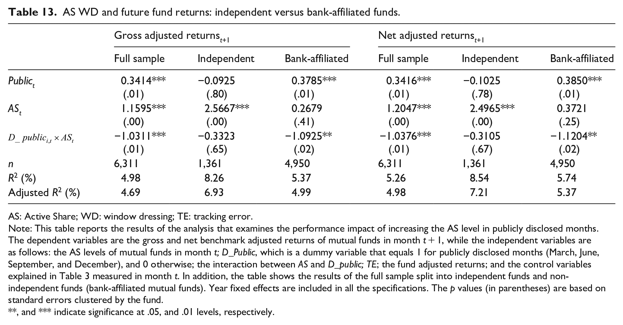
Table 13 shows the results of running equation (15) for the full sample and for independent and non-independent (bank-affiliated) subsamples. The results for the full subsample show that increasing the level of activity at quarter-ends negatively influences fund performance (coefficient of D_public^xAS), which confirms H3. Moreover, this negative impact is not observed in the independent funds subsample and only the bank-affiliated funds subsample shows a statistically significant coefficient on D_public^xAS. This result supports our intuition that the increase of AS in publicly disclosed months is probably related to informed trades for the independent funds subsample and probably related to WD for the non-independent funds subsample.

Table 13.

AS WD and future fund returns: independent versus bank-affiliated funds.

	Gross adjusted returnst+1			Net adjusted returnst+1
	Full sample	Independent	Bank-affiliated	Full sample	Independent	Bank-affiliated
Publict	0.3414*** (.01)	−0.0925(.80)	0.3785*** (.01)	0.3416*** (.01)	−0.1025(.78)	0.3850*** (.01)
ASt	1.1595*** (.00)	2.5667*** (.00)	0.2679(.41)	1.2047*** (.00)	2.4965*** (.00)	0.3721(.25)
$Dpubli{c}_{i,t}\times A{S}_t$	−1.0311*** (.01)	−0.3323(.65)	−1.0925** (.02)	−1.0376*** (.01)	−0.3105(.67)	−1.1204** (.02)
n	6,311	1,361	4,950	6,311	1,361	4,950
R2 (%)	4.98	8.26	5.37	5.26	8.54	5.74
Adjusted R2 (%)	4.69	6.93	4.99	4.98	7.21	5.37

AS: Active Share; WD: window dressing; TE: tracking error.

Note: This table reports the results of the analysis that examines the performance impact of increasing the AS level in publicly disclosed months. The dependent variables are the gross and net benchmark adjusted returns of mutual funds in month t + 1, while the independent variables are as follows: the AS levels of mutual funds in month t; D_Public, which is a dummy variable that equals 1 for publicly disclosed months (March, June, September, and December), and 0 otherwise; the interaction between AS and D_public; TE; the fund adjusted returns; and the control variables explained in Table 3 measured in month t. In addition, the table shows the results of the full sample split into independent funds and non-independent funds (bank-affiliated mutual funds). Year fixed effects are included in all the specifications. The p values (in parentheses) are based on standard errors clustered by the fund.

**

, and *** indicate significance at .05, and .01 levels, respectively.

Conclusion

In this study, we use a unique database that includes non-publicly disclosed portfolios to test whether mutual funds alter their holdings in publicly disclosed months to appear more active by reporting a high level of AS to attract future money flows. No study in the literature has examined whether the level of deviation from the benchmark can be altered by portfolio managers (AS WD). We compute how fund holdings deviate from the benchmarks using the AS metric of Cremers and Petajisto (2009).

We examine the relationship between AS and future fund performance, and the relationship between AS and money flows, and demonstrate that the higher the AS level, the higher the future fund returns and flows. Hence, we hypothesize that certain portfolio managers have incentives to show a high level of AS when the portfolios are publicly available. Therefore, we study the existence of AS WD and how this practice influences future fund performance and money flows. We define the AS_difference as the difference in the level of AS in publicly reported months as opposed to the level in the surrounding months and use it as a proxy for AS WD. We find that high AS_difference values are related to poor future fund performance but high future money flows.

Finally, we analyze funds that are more prone to conducting AS WD. We find that, contrary to the other categories of funds, on average, funds with high AS and low TE levels increase their AS levels before their holdings are public and reduce them afterward, hence showing a significant and positive AS_difference. Moreover, this category of funds exhibits the worst future performance but attracts higher money flows than funds with similar levels of TE. This finding also indicates that this strategy of deviating more from benchmarks when holdings are public makes economic sense because the higher the money flows are, the higher the incomes to the management companies, given that most Spanish mutual funds charge their fees based on TNA. However, we should not forget that these investment strategies conducted by certain funds erode investor fund performance, particularly in the case of bank-affiliated funds.

We believe that the results presented here are compelling enough to warrant further analysis. The above-mentioned results provide evidence of the implications of this research to policymakers who should consider the necessity of monthly portfolio holdings instead of quarterly holdings to limit the discretion of portfolio managers. Although we are aware of the difficulties in obtaining both publicly and non-publicly available portfolio holdings for all funds in a given investment category, future research in this area could extend this study to other countries in the eurozone and the US market. The existence of publicly and non-publicly available holdings for all mutual funds in the different eurozone countries will allow researchers to examine whether the AS WD phenomenon is just a characteristic of the Spanish market or if it is a widespread phenomenon. Another line of research could involve a more detailed analysis of the investors’ reactions, to examine whether they are aware of this managerial practice.