Sage Journals: Discover world-class research

Abstract

We evaluate the feasibility of estimating test-score growth for schools and districts with a gap year in test data. Our research design uses a simulated gap year in testing when a true test gap did not occur, which facilitates comparisons of district- and school-level growth estimates with and without a gap year. We find that growth estimates based on the full data and gap-year data are generally similar, establishing that useful growth measures can be constructed with a gap year in test data. Our findings apply most directly to testing disruptions that occur in the absence of other disruptions to the school system. They also provide insights about the test stoppage induced by COVID-19, although our work is just a first step toward producing informative school- and district-level growth measures from the pandemic period.

Keywords

assessment educational policy evaluation policy analysis regression analyses research methodology testing

Test-score growth is a commonly used evaluation tool in education research and policy applications. The abrupt cancellation of testing in spring 2020 due to COVID-19 generated a gap year in test data in states across the United States, a consequence of which is that it will not be possible to estimate traditional growth models in 2021. Motivated by this data condition, we assess the potential for reliably estimating test-score growth over a 2-year period with a gap year in testing.¹

Our methodological approach is to simulate a gap year in testing in a year preceding COVID-19. Specifically, we build a data panel spanning the school years 2016–2017, 2017–2018, and 2018–2019, and censor the data as if the 2017–2018 test was never administered. We estimate models of student test-score growth using the artificially censored data and compare the output with analogous output obtained using the full, uncensored data panel over the same 2-year period. These comparisons allow us to assess the accuracy of gap-year growth estimates relative to the full-data condition. Our simulations are not confounded by complicating factors associated with the test gap that occurred in reality due to the COVID-19 pandemic. This is appealing from the perspective of understanding the prospects for gap-year growth modeling in the absence of other complications. In the context of the pandemic—during which there have been many complications—our work is best viewed as providing evidence on a necessary, but not sufficient, condition for the resumption of useful growth modeling in spring 2021.

We focus primarily on determining the accuracy with which we can estimate test-score growth for districts and schools. Districts and schools are natural units of analysis from the perspective of state education agency staff interested in understanding variability in learning rates within their states. Moreover, although high-stakes growth measures from the pandemic period are unlikely to be used for accountability purposes, the historical use of district- and school-level growth estimates in this way has created inertia around metrics at these levels within state education agencies.² From a research perspective, growth-based analyses at the district and school levels are also commonly used to evaluate education interventions.

In our simulations, we find that gap-year models produce estimates of growth at the district and school levels that are highly correlated with estimates that use all the data. Specifically, the correlations are consistently around 0.90 for districts and range between 0.84 and 0.88 for schools, across five different growth model specifications in two subjects (math and English language arts [ELA]). We also extend our analysis to briefly consider a scenario where there is a 2-year test gap (in the case of COVID-19, this would be a situation where testing is further postponed to 2022). We do not believe that it will be feasible to estimate test-score growth for individual schools spanning a 2-year test gap, but we show that reasonably accurate district-level growth estimates can still be recovered.

Though we find broad similarity between the results obtained under the gap-year and full-data conditions, the estimates are not identical. For the differences that exist, we investigate their sources and identify two primary factors. First, the cohorts of students used to estimate growth in the gap-year and full-data scenarios only partially overlap. If we force cohort alignment in both scenarios, the correlations reported in the previous paragraph rise by about 0.05. Second, the remaining discrepancies are the result of what we refer to as data and modeling variance—that is, they arise because the gap-year model estimates growth from period t−2 to t, whereas the full-data analog sums single-year estimates of growth from t − 2 to t − 1 and t − 1 to t. This generates small differences in the predictors of contemporary achievement and their coefficients. We rule out other sources of the discrepant results due to the gap year. Most significantly, conditional on cohort-alignment, sampling variance at the individual student level does not meaningfully affect growth estimates for districts and schools using the gap-year data.

We also examine the extent to which differences in growth rankings caused by a gap year can be systematically predicted by observable district and school characteristics. We find that most of the variance in growth-ranking changes is not explained by observable characteristics. However, in sparser growth models, they explain a nonnegligible share of the variance—up to 25%. In our richest growth specification, the explained variance falls dramatically into the range of 1% to 5%. In a supplementary analysis, we show that a likely explanation for the difference is that estimates from the sparser models contain more bias.

Our findings speak directly to the ability of gap-year models to recover accurate growth estimates under normal circumstances, such as in the event of a technical or policy glitch that prevents testing in an otherwise typical school year. A recent example occurred in Tennessee in 2015–2016, when statewide testing in Grades 3 to 8 was cancelled due to problems with test delivery that ultimately resulted in the state terminating its contract with the test developer (Tatter, 2016). There is also the possibility that testing gaps will become more common in the future with increasing volatility around state testing policies.

In the context of COVID-19, in addition to the gap year in testing, the pandemic comes with a host of other challenges that must also be considered in efforts to use growth data effectively. Two in particular are notable. First, there will be changes in the composition of test-takers in public schools when testing resumes, and relatedly, the potential for changes to the composition of testing modes among students who are tested (e.g., in-person vs. online). Because uncertainty along these dimensions is so great and conditions vary so much across locales (e.g., see Donaldson & Diemer, 2021; Goldhaber et al., 2020), we do not attempt to address these issues directly in our simulations. However, to use growth data from the pandemic period effectively, researchers will need to account for missing and multimode test data.

The second challenge is that the pandemic has affected more than just schools, making the attribution of heterogeneity in growth across districts and schools more difficult. This challenge applies to the use of growth data for accountability and in some research projects. Noting these challenges, our work on the technical implications of the gap year is a necessary first step toward restarting the growth modeling infrastructure postpandemic.

Method

Growth Models

We estimate five different models in two subjects (math and ELA) to recover estimates of test-score growth for districts and schools. The models differ in terms of structure and the variables included as shown in Table 1 and were selected to be representative along key dimensions of many models used in practice. For instance, Model 3 is an example of what Koedel et al. (2015) refer to as a “standard one-step VAM [value-added model],” which is common in research and some policy applications, and Model 5 is similar in structure and variables to the two-step model that Parsons et al. (2019) favor for estimating teacher value-added. Models 1 and 2 share a key feature with student growth percentiles (SGPs)—which are commonly used in policy applications—in that they do not include any controls except lagged achievement.³

Table 1

Descriptions of the Five Growth Specifications

Growth specification	Sparse		Student controls		All controls
Growth specification	(1)	(2)	(3)	(4)	(5)
Structure	1-step	2-step	1-step	2-step	2-step
Student lagged test scores (math and ELA)	×	×	×	×	×
Individual student characteristics			×	×	×
School- and district-average student characteristics					×

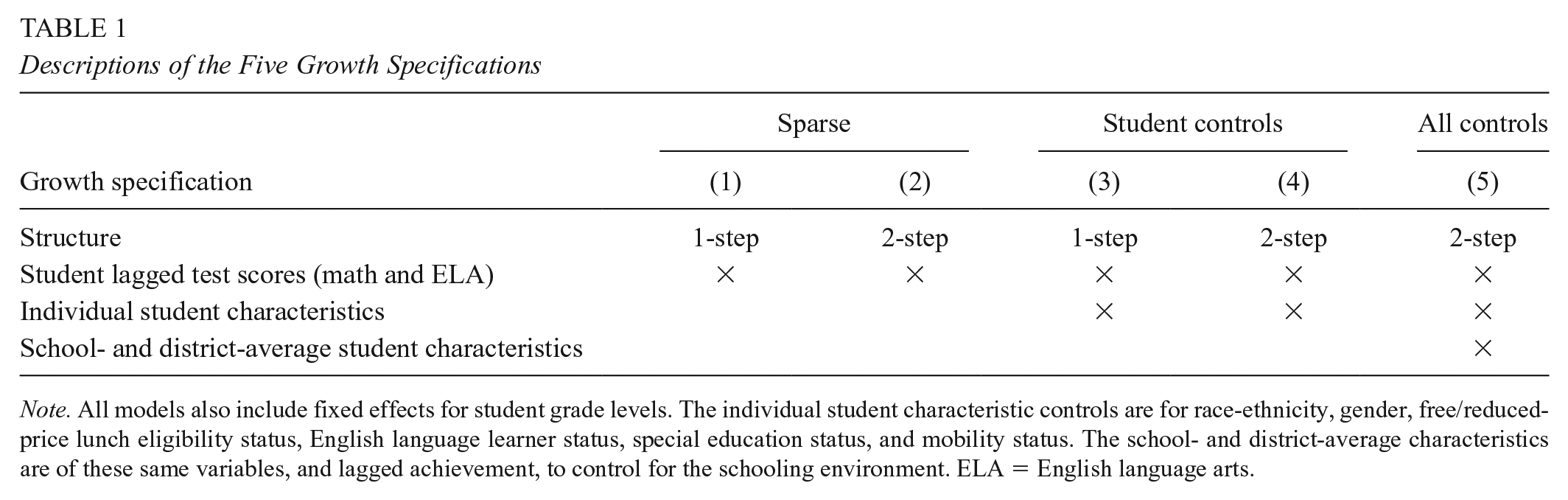
Note. All models also include fixed effects for student grade levels. The individual student characteristic controls are for race-ethnicity, gender, free/reduced-price lunch eligibility status, English language learner status, special education status, and mobility status. The school- and district-average characteristics are of these same variables, and lagged achievement, to control for the schooling environment. ELA = English language arts.

Examples of our fullest specifications, using one-step and two-step growth modeling structures, are shown in Equations (1) to (3). These specifications are commonly referred to as “value-added models”, or VAMs, in the literature. The term value-added implies attribution of growth to the units of analysis—in our case, schools or districts. However, the models can provide useful information about growth differences between schools and districts even in the absence of attribution. Put another way, they can be used diagnostically to identify heterogeneity in rates of student achievement growth across districts and schools even when it is uncertain how much of the differences can be reasonably attributed to the actions of districts and schools themselves. In the discussion section below, we elaborate further on the use of growth models for diagnostic and evaluation purposes.⁴

Our full specification for the one-step model is shown by Equation (1):

Y_{i j k m s t} = α_{0} + Y_{i m t_1} α_{1} + X_{i t} α_{2} + γ_{j} + φ_{s} + e_{i j k m s t}

(1)

Equations (2) and (3) show the full specification for the two-step model:

\begin{array}{l} Y_{i j k m s t} = β_{0} + Y_{i m t_1} β_{1} + X_{i t} β_{2} + {\bar{Y}}_{m s t_1} β_{3} + {\bar{Y}}_{m k t_1} β_{4} \\ + {\bar{X}}_{s t} β_{5} + {\bar{X}}_{k t} β_{6} + ψ_{j} + ε_{i j k m s t} \end{array}

(2)

ε_{i j k m s t} = π_{s} + u_{i j k m s t}

(3)

In Equations (1) and (2), $Y_{i j k m s t}$ is the standardized test score of student i in grade j, attending school s, in district k, for subject m, and year t. $Y_{i m t_1}$ is a vector of lagged-test-score controls, of which the key controls are the same-subject and off-subject lagged test scores.⁵ In Equation (2), the vectors ${\bar{Y}}_{m s t_1} and {\bar{Y}}_{m k t_1}$ include school and district average values of the lagged test-score variables. In the gap-year models, t−1 scores are unavailable and t−2 scores are substituted.

The vector $X_{i t}$ contains student characteristics. We include indicator variables for student race/ethnicity, gender, free or reduced-price lunch (FRL) status, English language learner status, whether the student has an individualized education program (IEP), and mobility status (i.e., an indicator for whether the student changed schools midyear). We also include the school and district shares of these variables in the vectors ${\bar{X}}_{s t}$ and ${\bar{X}}_{k t}$ in Equation (2). $γ_{j}$ and $ψ_{j}$ are grade fixed effects. As written in Equations (1) and (3), $φ_{s}$ and π_s are school fixed effects. These are our estimates of school-level growth. Note that when we rerun the models to recover district-level growth estimates, we replace the school fixed effects with district fixed effects (i.e., with subscripts “k” instead of “s”), reestimate the models, and recover these parameter estimates instead. $e_{i j k m s t}$ , $ε_{i j k m s t}$ , and $u_{i j k m s t}$ are the error terms.

The versions of the models shown by Equations (1) to (3) are labeled as “Model 3” and “Model 5” in Table 1. Models 1 and 2 in Table 1 are sparse versions of the one-step and two-step models—they include only the $Y_{i m t_1}$ vector and the grade fixed effects. Model (4) is a two-step model that includes all the information in the full one-step model shown in Equation (1)—that is, it includes all student-level controls but excludes all district- and school-aggregated information. Note that the school- and district-aggregate coefficients are not separately identified in a one-step model because there is no within-unit (school or district) variation in the aggregate covariates. This is why we do not estimate a one-step model with these controls. The two-step model “resolves” the identification problem by estimating the parameters sequentially. It is beyond the scope of the current article to go into details on the technical and policy trade-offs of the various models, but Ehlert et al. (2016) and Parsons et al. (2019) provide conceptual and technical arguments for why a 2-step model with rich controls along the lines of Model (5) is desirable.⁶

We link student growth to the contemporary school or district in all models as a baseline condition. This is the common approach under normal circumstances—that is, growth from year-(t − 1) to year-t is linked to the year-t school or district. In the gap-year model, this is a potential concern because there is extra mobility during the gap year. We examine the sensitivity of gap-year model output to adjustments for student mobility over the course of our analysis.

The last estimation issue that merits brief mention is shrinkage. All of our estimates are shrunken toward the mean using the following procedure described in Koedel et al. (2015), which is implemented in two steps. First, for each school or district estimate, we produce an estimate-specific shrinkage factor, $α$ . For each school s, the shrinkage factor is written as

α_{s} = \frac{{\hat{σ}}^{2}}{{\hat{σ}}^{2} + {\hat{λ}}_{s}}

(4)

In the formula, ${\hat{σ}}^{2}$ is an estimate of the variance of true growth across schools in the sample (after netting out estimation error), and ${\hat{λ}}_{s}$ is the estimation-error variance of the estimate for school s.⁷ These shrinkage factors can be thought of as individual school (or district) reliability ratios that reflect the precision of each estimate in the context of the total true variance in growth.

With the shrinkage factors in hand, the final, shrunken growth estimates are calculated as (again, the formula for schools is shown but the formula for districts is analogous):

{\tilde{φ}}_{s} = α_{s} {\hat{φ}}_{s} + (1 - α_{s}) \bar{φ}

(5)

where ${\hat{φ}}_{s}$ is estimated growth for school s and $\bar{φ}$ is average growth across all schools. Equation (5) embodies the intuitive idea that as the estimate for any individual school s becomes less precise, as measured by $α_{s}$ , we put more weight on the prior that the school has average growth.

As a final note to this section, the connection between the growth estimates from our models and SGPs merits additional explanation given the widespread use of SGPs by states to measure growth (Data Quality Campaign, 2019). SGPs are estimated using quantile regression and aggregated for schools and districts as median values of individual students’ growth percentiles. In addition to using quantile regression and focusing on the median rather than the mean, SGPs differ from the models we estimate in that they condition only on lagged achievement in a single subject (with no other controls), use multiple years of lagged test scores for students when available, and are based on simple aggregations of the data without shrinkage.

Several previous studies have compared output from SGPs with output from linear growth models similar to ours (Castellano & Ho, 2015; Ehlert et al., 2016; Goldhaber et al., 2014). A general expectation based on these studies is that SGPs should be affected by the gap year similarly to growth estimates from our Models 1 and 2, which also condition only on lagged student achievement and exclude other controls. For example, Castellano and Ho (2015) and Ehlert et al. (2016) show that SGPs and growth estimates from linear models are similar when based on the same lagged-achievement controls (with correlations at or above 0.90). If anything, SGPs should be expected to be slightly more sensitive to a gap year in testing than our estimates from Models 1 and 2 because (a) they are less efficient than mean-based growth estimates (Castellano & Ho, 2015) and (b) there is nothing akin to our ex post shrinkage procedure applied to SGPs.⁸ As a point of related evidence, Goldhaber et al. (2014) show that teacher-level SGPs have lower year-to-year stability than growth estimates from linear models.

Gap-Year Simulation

We estimate each model described above with and without simulating a gap year in testing. We begin by using the uncensored data to estimate two consecutive growth estimates for each unit (either a school or a district) with data from 2016–2017 to 2017–2018, and 2017–2018 to 2018–2019. We then sum the two single-year estimates to produce an estimate of growth over the 2-year period in order to replicate how a typical system would estimate growth over 2 years, assuming no data were missing. Next, we censor the 2017–2018 test data and directly estimate growth over the 2-year period, using data from 2016–2017 and 2018–2019. By comparing the “full data” scenario with the “gap-year” scenario, we can assess the extent to which the gap-year models recover accurate estimates of test-score growth over the 2-year period.

We focus primarily on comparing full-data and gap-year growth estimates for districts and schools over the same 2-year timespan. In addition, we compare the gap-year growth estimates with growth estimates from only the most recent year—that is, in the context of our simulations, we estimate gap-year growth from 2016–2017 to 2018–2019 and compare it with growth from 2017–2018 to 2018–2019. This supplementary comparison is informative if policymakers were interested in using gap-year growth to approximate the most recent year of growth, for which a rationale might be a rigid accountability framework that does not permit the consideration of multiple years of growth. Ultimately, we do not emphasize this comparison for two reasons. First, it is not directly informative about the performance of the gap-year model because the comparison is confounded by real differences in growth rates between schools and districts in the nonoverlapping year. Second, outside a rigid accountability framework, there is not a strong research or policy rationale for ignoring the first year of the 2-year window in the event of a gap year in testing.

Finally, we also briefly extend our analysis to simulate the presence of two consecutive gap years in testing—in the context of the COVID-19 pandemic, this scenario would come to pass if testing does not resume until spring 2022. For this extension, we bring in an earlier year of data from 2015–2016, censor the test data in our panel in 2016–2017 and 2017–2018, and calculate growth from 2015–2016 to 2018–2019. We then compare growth estimated over the 3-year period with the analogous “full data” condition, where 3-year growth is calculated as the sum of annual growth estimates from 2015–2016 to 2016–2017, 2016–2017 to 2017–2018, and 2017–2018 to 2018–2019.

Data

We use administrative microdata from Missouri covering all students tested in Grades 3–8 in math and ELA during the school years 2015–2016 to 2018–2019. Hereafter, we identify school years by the spring year—for example, 2018–2019 as 2019. We standardize student test scores throughout by grade-subject-year. Supplemental Appendix Table A1 (available in the online version of this article) reports student-level correlations of test scores over time in math and ELA, which can be used by other states to get a rough sense of the likely generalizability of our findings to other assessment contexts. As a related point of information, the test reliability ratios in Missouri are at or above 0.90 in most tested grades and subjects, typical of large-scale state tests elsewhere.⁹

We do not expect contextual features of Missouri to limit the generalizability of our findings in most respects. That said, two aspects of the Missouri data merit brief attention. First, Missouri changed its math and ELA tests once each between 2016 and 2019. Backes et al. (2018) studied the impact of test-regime changes on value-added estimates in math and ELA across multiple states and found that such changes typically do not affect model performance substantively. Moreover, we have performed internal diagnostic work using the Missouri data specifically that supports this inference.¹⁰

Second, Missouri has a high ratio of districts to students. Said another way, Missouri is a “small district” state. Growth estimates for smaller districts will be more sensitive to data changes because they have fewer students to balance out the sampling variance that the data changes create. These data changes can be of two types. First is the imperfect overlap of the samples between the full-data and gap-year scenarios, both at the cohort and individual-student levels.¹¹ Second, even with perfect overlap of students in the full-data and gap-year scenarios, differences in the same students’ test scores in the t − 1 and t − 2 years can affect the growth estimates. We conduct a subsample analysis for the 100 largest districts in Missouri—in which these data changes are less impactful owing to their size—to produce results that are more likely to generalize to states with larger school districts.

We produce growth estimates for all districts and schools with at least 10 tested students. When we correlate and otherwise compare growth estimates using the full data and gap-year data, the comparisons are restricted to districts and schools that meet the size threshold in both data conditions. Only very small Missouri districts and schools are omitted from our analysis due to the sample-size restriction.¹²

Table 2 summarizes our data in terms of students, schools, and districts.

Table 2

Summary Statistics for Students, Schools, and Districts in the Analytic Sample

School/student/district information	M	SD
Student information
Standardized math score	0.02	0.99
Standardized ELA score	0.02	0.99
Asian	0.02	0.14
Black	0.16	0.36
Hispanic	0.07	0.25
White	0.71	0.45
Multiple and other race/ethnicity	0.04	0.20
Female	0.49	0.50
Eligible for free/reduced-price lunch	0.52	0.50
English language learner	0.05	0.22
Individualized education program	0.13	0.34
Mobile student	0.04	0.20
School information
Urban	0.18	0.38
Suburban	0.24	0.43
Rural/town	0.59	0.49
Enrollment	357	217
District information
Enrollment (all)	1603	3194
Average number of schools (all)	4.2	6.1
Enrollment (large district subsample)	6321	5333
Average number of schools (large district subsample)	12.4	11.0
N (student years, 2017–2019)	972,877
N (unique schools, 2017–2019)	1,730
N (unique districts, 2017–2019)	557

Note. These summary statistics are based on the analytic sample of students in Grades 4–8 in 2016–2017, 2017–2018, and 2018–2019 who have lagged test scores and attend districts and schools with at least 10 test takers. Urbanicity information is taken from the 2018–2019 Common Core of Data. The large-district subsample is selected to include the 100 districts in Missouri with the largest populations of test-takers included in the gap-year model. Other size-based selection criteria produce a similar sample; we chose this criterion to isolate districts in Missouri with the largest samples relevant for our primary analysis. ELA = English language arts.

Results

Assessing the Alignment Between Gap-Year and Full-Data Growth Estimates

We estimate district- and school-level growth using the full data, then using the censored data as if the 2018 test was not administered and compare the results by estimating the correlation between the growth estimates. Each cell in Table 3 shows one such correlation between school- or district-level growth estimates, with and without the data censoring, defined by three dimensions: (1) the subject (math or ELA) and model (Models 1–5) indicated by the column, (2) the level of the analysis (district or school) indicated by the two horizontal panels, and (3) the precise data and evaluation condition, identified by the rows within each horizontal panel.

Table 3

Correlations Between Gap-Year and Full-Data Growth Model Output Using Different Models and Different Data and Estimation Conditions

Models	Math					ELA
Models	Model 1	Model 2	Model 3	Model 4	Model 5	Model 1	Model 2	Model 3	Model 4	Model 5
District models
Baseline	0.91	0.91	0.90	0.90	0.90	0.88	0.88	0.88	0.89	0.90
Same cohorts	0.95	0.95	0.95	0.95	0.96	0.94	0.94	0.94	0.94	0.96
Same students	0.96	0.96	0.95	0.96	0.96	0.95	0.95	0.95	0.95	0.97
Mobility adjustment 1 (to baseline): omit movers	0.90	0.90	0.89	0.89	0.90	0.87	0.87	0.87	0.87	0.89
Mobility adjustment 2 (to baseline): 50-50 mover credit	0.90	0.90	0.90	0.90	0.91	0.88	0.88	0.88	0.88	0.90
School models
Baseline	0.88	0.87	0.87	0.87	0.85	0.86	0.85	0.85	0.84	0.84
Same cohorts	0.91	0.92	0.91	0.92	0.90	0.89	0.89	0.89	0.89	0.89
Same students	0.91	0.92	0.91	0.92	0.90	0.89	0.89	0.89	0.89	0.90
Mobility adjustment 1 (to baseline): omit movers	0.88	0.86	0.87	0.85	0.84	0.86	0.83	0.86	0.83	0.83
Mobility adjustment 2 (to baseline): 50-50 mover credit	0.89	0.87	0.88	0.86	0.87	0.87	0.85	0.87	0.84	0.85

Note. Each cell shows a correlation coefficient between growth measures using the gap-year and full-data scenarios. ELA = English language arts.

Our baseline findings for districts and schools are reported in the first row of each horizontal panel. The two key features of the baseline condition, both of which we relax subsequently, are (a) we compare the gap-year and full-data results using all available data in each condition and (b) we assign growth over the previous period—be it one (t−1) or two (t−2) years—to the year-t district or school, which is the business-as-usual approach in the absence of a gap year. The results for districts show that the gap-year estimates are highly correlated with the full-data estimates in both subjects. The correlations are consistently around 0.90 and slightly higher in math. The correlations are a little lower for individual schools—in the range of 0.84–0.88 across models and subjects—but substantively similar.¹³

A high-level takeaway from the baseline correlations is that they indicate a strong correspondence between growth estimated with and without the gap year, regardless of level of analysis, growth model, or subject. In the online Supplemental Appendix Table A2, we provide complementary transition matrices corresponding to the baseline correlations. Reflecting the fact that research and policy interest is often concentrated in the tails of the distribution, the transition matrices examine the persistence of district and school placements in the “bottom 10%,” “middle 80%,” and “top 10%” of growth rankings with and without the gap year. Mirroring the high correlations in Table 3, the transition matrices show that most districts and schools (about 85%–88%) remain in the same ranking category regardless of whether the full data or gap-year data are used. Moreover, as expected, the districts and schools that change categories are relatively close to the 90th- and 10th-percentile cutoffs, on average; among these districts and schools, the average value of the percentile ranking change caused by the gap year of data is about 10 percentile points—for example, a move from the 85th to 95th percentile.

Noting that the baseline correlations are generally high, one might still wonder why they are not even higher. After all, both the gap-year and full-data models aim to recover growth estimates over the same 2-year period. Understanding what factors drive differences between the estimates is important for understanding the limitations of using gap-year data.

In the second and third rows in each panel of Table 3, we explore the extent to which changes in the analytic sample between the gap-year and full-data models can explain differences in the results. In the second row, we force the gap-year and full-data models to be estimated on the same cohorts of students. In the baseline condition, the full-data models include some cohorts that are not represented in the gap-year models. As an example, consider a student in the third grade during the gap year, which for us is 2018. Her growth contributes to estimates from 2018 to 2019 in the full data condition, but because she is outside the tested range prior to 2018 (i.e., in 2017, she is in the second grade), her growth cannot be assessed with the gap-year model. A similar problem arises for students in the eighth grade during the gap year, who age out of the testing window before testing resumes.

When we force cohort alignment between the models, the correlations in all scenarios rise markedly, on the order of about 0.05 off of the already high baseline values. This indicates that cohort misalignment between the gap-year and full-data conditions accounts for a substantial fraction of the result discrepancies. This finding is not likely to be policy actionable because in the presence of a true gap year, the missing cohorts will simply not have data. However, it is instructive about why the growth estimates differ.

Next, in the third row in each panel of Table 3, we further align the samples across the gap-year and full-data conditions by using the exact same students to estimate the models. That is, conditional on cohort alignment, we further exclude all students within the matched cohorts that do not have a test score for all three years (2017, 2018, and 2019). The results show that conditional on matching cohorts, matching the exact student samples has a negligible effect. The correlations do increase when we fix the samples, but the increase is very small and in some cases not detectable up to the 100th decimal place.

Another way in which the gap-year and full-data models differ is in how they treat mobile students. To illustrate, consider a student who attends District A in 2017 and 2018, but District B in 2019. In the business-as-usual model, her growth from 2017 to 2018 will be attributed to District A, and her growth from 2018 to 2019 will be attributed to District B. However, in the gap-year model and using the convention of assigning growth to the contemporary district, her growth over the full 2-year period will be attributed to District B.

We assess the extent to which two different mobility-based adjustments to the gap-year model improve its performance. First, we drop students from the gap-year model who were not enrolled in the same district (or school) in period t−1 and t—that is, in 2018 and 2019 in our dataset. These students only attended the contemporary district (or school) for one of the two years over which gap-year growth is estimated, meaning that their full-period growth is partly misattributed using the convention of assigning growth to the contemporary location. In the second mobility modification, we retain mobile students in the gap-year dataset but assign 50% weight to the districts (or schools) attended in 2018 and 2019, respectively.¹⁴

The results in Rows 4 and 5 of each panel of Table 3 show the correlations after making the mobility adjustments to the gap-year models. The correlations otherwise maintain the baseline evaluation conditions, so the effects of the mobility adjustments can be inferred by comparing the results with the results in Row 1. For districts, neither mobility adjustment results in an improvement in the performance of the gap-year model. In fact, the adjustment where we drop mobile students altogether (weakly) reduces the ability of the gap-year model to recover the full-data growth estimates. The reason is that the lost data reduces efficiency, offsetting any (very modest) gains owing to the reduced misattribution of mobile students’ growth.

For schools, the strategy of dropping the data for movers also performs (weakly) worse for the same reason. However, the 50-50 weighting strategy modestly improves estimation accuracy in the gap-year model. A reason why the results differ between districts and schools—albeit only slightly—is that there are many more school than district movers during the gap year.¹⁵

In the online Supplemental Appendix Table A3, we replicate the analyses in Table 3 for the subsample of the 100 largest districts in Missouri, noting that these findings will be more generalizable to “large district” states. The findings are substantively similar to our results for all districts in Table 3, although the baseline correlations are higher owing to the larger sample sizes.

In summary, Table 3 shows that cohort misalignment is the single largest observable factor that drives down the baseline correlations between the gap-year and full-data growth estimates. In the school-level models, differences in how the full-data and gap-year models attribute growth for mobile students is also a small contributing factor. We are left to conclude that the remaining discrepancies arise from data and modeling variance.¹⁶ Again, this variance stems from the fact that we model growth from t − 2 to t − 1 and from t − 1 to t in the full-data models, and directly from t−-2 to t in the gap-year models. Individual students’ t − 1 and t − 2 test scores are different (data variability), and the model coefficients on the t − 1 and t − 2 test scores are different, which in turn can affect other coefficients in the models (modeling variability). As unit-level (district or school) sample sizes become large, the effect of the data variability shrinks, but the effect of modeling variability does not.

Finally, in Table 4, we briefly show results from our supplementary comparison of the gap-year growth estimates to growth during only the most recent year—from 2018 to 2019. The reporting in Table 4 follows the same structure in Table 3, although we omit the mobility-adjusted estimates for brevity. The correlations in Table 4 are uniformly lower than in Table 3, with average declines in the district- and school-level analyses across models and subjects of 0.09 and 0.07 correlation points, respectively. The lower correlations are unsurprising because in addition to the above-documented comparability issues, there is also misalignment between the periods over which growth is measured. The correlations in Table 4 that decline the most are for Model 5, which is the most comprehensive model. An explanation is that Model 5 includes the richest control-variable set (and perhaps is overcontrolled, per Parsons et al., 2019), which limits the scope for correlated bias in the growth estimates covering the different (albeit overlapping) time spans.

Table 4

Correlations Between Gap-Year Growth Model Output and Growth Model Output Using Data From Just the Most Recent Year (2018 to 2019 in Our Simulations) Using Different Models and Data

Models	Math					ELA
Models	Model 1	Model 2	Model 3	Model 4	Model 5	Model 1	Model 2	Model 3	Model 4	Model 5
District models
Baseline	0.86	0.85	0.86	0.86	0.76	0.80	0.80	0.81	0.81	0.77
Same cohorts	0.88	0.87	0.89	0.89	0.80	0.82	0.81	0.83	0.83	0.79
Same students	0.89	0.88	0.90	0.89	0.80	0.81	0.81	0.83	0.83	0.78
School models
Baseline	0.86	0.84	0.86	0.84	0.77	0.82	0.79	0.82	0.79	0.74
Same cohorts	0.87	0.84	0.88	0.86	0.80	0.80	0.76	0.81	0.78	0.74
Same students	0.87	0.85	0.88	0.86	0.80	0.80	0.76	0.81	0.78	0.74

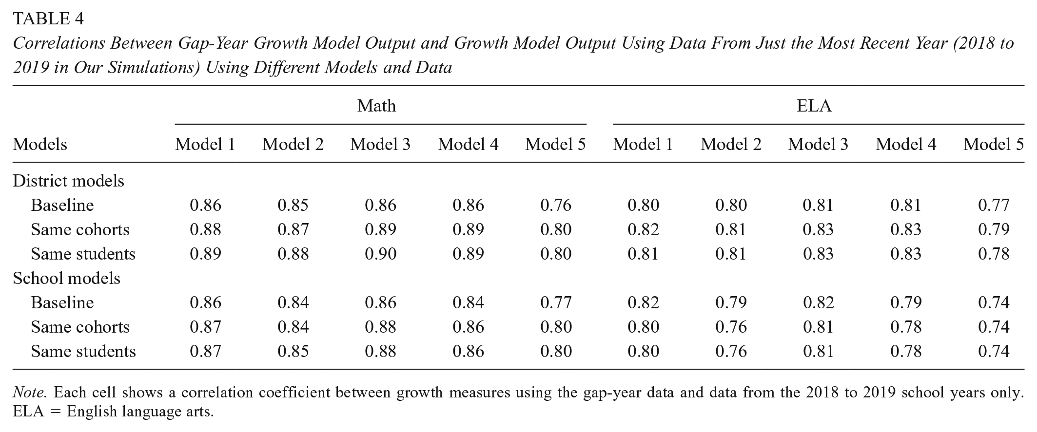
Note. Each cell shows a correlation coefficient between growth measures using the gap-year data and data from the 2018 to 2019 school years only. ELA = English language arts.

Factors That Predict Changes in Growth Rankings Induced by the Gap Year

Next, we assess whether observable district and school characteristics predict ranking changes between the gap-year and full-data models under the baseline estimation conditions. Tables 5 and 6 show results from regressions where the dependent variable is the difference in growth rankings between the gap-year and full-data models—that is, we estimate each model separately, assign districts and schools percentile ranks based on the growth estimates, and subtract the full-data percentile from the gap-year percentile. The independent variables are district and school characteristics including the 2017 same-subject achievement level, the number of test takers, and student shares by race-ethnicity, gender, FRL, English as a second language, participation in an IEP, and student mobility (in particular, the share of tested students who experienced a midyear school move). All the independent variables are standardized to have a mean of zero and a variance of one—within the district or school distribution depending on the level of analysis—which allows the coefficients to be interpreted in (common) standard deviation units throughout.

Table 5

Observable Predictors of Changes to District Growth Rankings (in Percentiles) Due to the Gap Year in Testing

Predictors	Math					ELA
Predictors	Model 1	Model 2	Model 3	Model 4	Model 5	Model 1	Model 2	Model 3	Model 4	Model 5
Period t − 2 test-score level (same subject)	−7.76* (0.75)	−7.52* (0.76)	−8.30* (0.81)	−8.06* (0.81)	2.36* (0.79)	−5.83* (0.82)	−5.41* (0.83)	−7.09* (0.84)	−6.74* (0.83)	2.02* (0.77)
Period t − 2 percent Asian	−0.18 (0.68)	−0.17 (0.68)	−0.13 (0.60)	−0.07 (0.59)	0.17 (0.81)	−0.53 (0.75)	−0.46 (0.78)	−0.32 (0.85)	−0.21 (0.85)	0.61 (0.77)
Period t − 2 percent Black	−1.37* (0.61)	−1.37* (0.61)	−2.23* (0.71)	−2.35* (0.70)	−0.57 (0.63)	−1.21* (0.61)	−1.19* (0.60)	−2.22* (0.63)	−2.15* (0.63)	0.06 (0.65)
Period t − 2 percent Hispanic	−0.68 (1.41)	−0.73 (1.46)	−1.04 (1.42)	−0.86 (1.48)	−0.58 (1.54)	−2.03 (1.38)	−2.08 (1.40)	−2.38 (1.39)	−2.32 (1.37)	−0.68 (1.37)
Period t−2 percent other race	0.55 (0.61)	0.47 (0.61)	0.16 (0.63)	0.12 (0.63)	0.55 (0.70)	−0.50 (0.80)	−0.48 (0.81)	−0.47 (0.81)	−0.39 (0.80)	0.08 (0.76)
Period t − 2 percent female	−0.71 (0.61)	−0.67 (0.62)	−1.22* (0.65)	−1.21 (0.65)	−1.77* (0.76)	−0.01 (0.77)	0.05 (0.76)	0.18 (0.71)	0.19 (0.70)	−0.42 (0.72)
Period t−2 percent FRL	−1.65* (0.80)	−1.75* (0.81)	−2.73* (0.88)	−2.99* (0.88)	1.07 (0.88)	−0.21 (0.85)	−0.28 (0.85)	−1.82* (0.86)	−2.31* (0.85)	0.18 (0.81)
Period t − 2 percent ESL	1.12 (1.40)	1.02 (1.45)	1.13 (1.43)	0.84 (1.49)	0.94 (1.67)	1.92 (1.47)	1.93 (1.50)	1.39 (1.47)	1.41 (1.45)	1.16 (1.39)
Period t − 2 percent IEP	−1.23* (0.49)	−1.15* (0.50)	−2.42* (0.65)	−2.33* (0.66)	0.46 (0.71)	−1.19* (0.52)	−1.07* (0.52)	−2.01* (0.54)	−1.90* (0.54)	0.66 (0.63)
Period t − 2 percent mobile	−1.80* (0.65)	−1.75* (0.66)	−1.63* (0.71)	−1.65* (0.72)	0.80 (0.69)	−0.47 (0.72)	−0.38 (0.73)	−0.39 (0.72)	−0.37 (0.72)	1.93* (0.68)
Number of test takers	−0.14 (0.47)	−0.09 (0.48)	0.03 (0.48)	0.02 (0.47)	−0.14 (0.47)	−1.37* (0.47)	−1.43* (0.47)	−1.46* (0.54)	−1.42* (0.55)	−0.93 (0.50)
R ²	0.247	0.229	0.242	0.233	0.054	0.160	0.140	0.176	0.158	0.039
N	540	540	540	540	540	540	540	540	540	540

Note. The dependent variable in these regressions is each district’s percentile ranking in the distribution of growth estimates using the gap-year data minus the percentile ranking using the full data. All variables are in standard deviations of the district distribution in period (t−2), which is 2017. FRL = free or reduced-price lunch; IEP = individualized education program; ELA = English language arts; ESL = English as a second language.

Indicates statistical significance at the 5% level or higher.

Table 6

Observable Predictors of Changes to School Growth Rankings (in Percentiles) Due to the Gap Year in Testing

Predictors	Math					ELA
Predictors	Model 1	Model 2	Model 3	Model 4	Model 5	Model 1	Model 2	Model 3	Model 4	Model 5
Period t − 2 test-score level (same subject)	−7.00* (0.580)	−7.20* (0.589)	−7.14* (0.582)	−7.54* (0.610)	3.26* (0.652)	−6.69* (0.67)	−5.91* (0.70)	−7.11* (0.69)	−6.44* (0.72)	1.46* (0.73)
Period t − 2 percent Asian	1.17* (0.547)	0.52 (0.546)	1.21* (0.544)	0.88 (0.562)	0.77 (0.619)	1.74* (0.57)	1.12 (0.58)	1.62* (0.57)	1.23* (0.59)	0.48 (0.62)
Period t − 2 percent Black	5.66* (2.685)	0.07 (2.776)	5.65* (2.696)	1.23 (2.840)	2.88 (3.163)	8.25* (2.79)	5.17 (3.12)	8.46* (2.79)	5.64 (3.11)	2.27 (3.15)
Period t − 2 percent Hispanic	3.66* (1.257)	1.74 (1.296)	3.71* (1.267)	2.48 (1.331)	1.75 (1.504)	4.35* (1.37)	2.55 (1.45)	4.58* (1.39)	2.70 (1.46)	1.81 (1.45)
Period t − 2 percent other race	9.07* (2.884)	1.71 (2.985)	9.46* (2.889)	3.82 (3.047)	3.68 (3.403)	12.57* (3.02)	8.11* (3.37)	12.97* (3.01)	8.99* (3.35)	2.86 (3.39)
Period t − 2 percent female	−0.53 (0.413)	−0.60 (0.400)	−0.68 (0.418)	−0.82* (0.412)	−0.80 (0.478)	0.08 (0.44)	−0.02 (0.47)	−0.25 (0.44)	−0.27 (0.47)	−0.53 (0.49)
Period t − 2 percent FRL	−0.72 (0.518)	−1.10* (0.533)	−1.02 (0.533)	−1.93* (0.561)	2.89* (0.616)	0.61 (0.61)	0.78 (0.66)	0.33 (0.63)	−0.59 (0.68)	1.29 (0.69)
Period t − 2 percent ESL	−1.40 (0.756)	−1.27 (0.769)	−1.53* (0.765)	−1.62* (0.785)	−0.59 (0.982)	−1.65 (0.93)	−0.78 (0.88)	−2.33* (0.98)	−1.39 (0.93)	−1.11 (0.91)
Period t − 2 percent IEP	−1.80* (0.423)	−1.67* (0.427)	−2.08* (0.417)	−2.09* (0.425)	0.55 (0.491)	−1.82* (0.45)	−1.75* (0.45)	−2.55* (0.43)	−2.68* (0.46)	−0.20 (0.51)
Period t − 2 percent mobile	−1.37* (0.390)	−1.40* (0.470)	−1.06* (0.442)	−0.88 (0.560)	1.70* (0.654)	−0.81 (0.47)	−0.40 (0.48)	−0.50 (0.54)	0.11 (0.55)	1.60* (0.60)
Number of test takers	2.67* (0.292)	−0.10 (0.306)	2.91* (0.295)	0.05 (0.311)	0.53 (0.365)	2.90* (0.32)	−0.17 (0.35)	3.03* (0.32)	−0.14 (0.35)	0.42 (0.37)
R ²	0.149	0.128	0.152	0.119	0.037	0.141	0.100	0.159	0.097	0.013
N	1,527	1,527	1,527	1,527	1,527	1,527	1,527	1,527	1,527	1,527

Note. The dependent variable in these regressions is each school’s percentile ranking in the distribution of growth estimates using the gap-year data minus the percentile ranking using the full data. All variables are in standard deviations of the school distribution in period (t−2), which is 2017. FRL = free or reduced-price lunch; IEP = individualized education program; ESL = English as a second language; ELA = English language arts.

Indicates statistical significance at the 5% level or higher.

We begin by focusing on the R² values, which give a summary indication of the predictive power of observable characteristics over gap-year-induced changes to growth rankings. For the growth estimates from Models 1 to 4, the R² values indicate that a nonnegligible fraction of the variance in ranking changes can be explained by observable district and school characteristics— about 14% to 25% for districts and 10% to 16% percent for schools. Alternatively, in Model 5, our fullest specification, observable district and school characteristics explain much less of the variance in ranking changes—about 4% to 5% for districts and 1% to 4% for schools.

The primary predictor of the rank changes in all models and subjects is the 2017 achievement level. The consistently negative coefficients on that variable using the estimates from Models 1–4 indicate that higher achieving districts and schools are adversely affected in growth rankings by the presence of the gap year, compared with the full-data analog. The magnitudes of the relationships are moderate, with a one standard deviation increase in the 2017 achievement level corresponding to a ranking reduction of about 5 to 8 percentile points. Noting that achievement levels can be viewed as indicators of socioeconomic advantage, it also bears mentioning that the coefficients on some of the other control variables in the multivariate regressions temper the relationship between socioeconomic advantage and lower rankings, on net.¹⁷ Still, on the whole, the lagged test-score coefficient dominates all of these, and the end result is that moving from the full data condition to the gap-year data condition in Models 1 to 4 systematically lowers estimated growth for socioeconomically advantaged districts and schools.¹⁸

A theoretical explanation for the findings from Models 1–4 is provided in the online Supplemental Appendix B. The appendix shows that the findings are consistent with the presence of modest omitted variables bias in the underspecified growth models. This bias is fully compounded in the consecutive single-year estimates used in the full-data scenario but partially attenuated in the gap-year estimates. The bias explanation is consistent (conceptually and directionally) with the bias documented in underspecified VAMs in Parsons et al. (2019) and implies that the gap-year estimates are less biased than their full-data counterparts. We caution that this does not mean that the gap-year estimates from the underspecified models are preferred because they have other limitations, most notably in terms of coverage and sample sizes.¹⁹

The finding that changes to the growth rankings based on Model 5 are not meaningfully explained by observable district and school characteristics, combined with the derivations in the online Appendix B, is consistent with that model producing the least-biased growth estimates. However, the evidence is not conclusive because Model 5 has the potential to overcorrect for student and school circumstances. Previous research suggests that overcorrection bias in fully controlled 2-step models, like Model 5, is more problematic in theory than in practice, but it is beyond the scope of the present article to delve into these details further. We refer interested readers to Ehlert et al. (2016) and Parsons et al. (2019) for more information.

Extension (2-Year Gap)

In this section, we briefly consider the prospects for estimating growth for schools and districts if there is a 2-year test gap. In our data, we simulate this situation by adding a year to the front end of our data panel and further censoring the data to remove the 2017 test. In this scenario, our view is that school-level growth metrics cannot be feasibly estimated. This is because most schools would not have any students who take both the pre- and postgap tests in the same building, which would require schools to cover four consecutive grades in the tested span (Grades 3–8). For example, third-grade students in a K–5 school in the pregap year would be sixth graders in a new school after a 2-year gap.²⁰ Complex and assumptive models could theoretically recover estimates of test-score growth for individual schools even in the absence of “fully contained” cohorts to anchor the estimates, but without considerable validity testing, we do not view this as a promising strategy.

Alternatively, district-level growth estimates with a 2-year gap can be feasibly estimated because most districts span four consecutive grades in the 3 to 8 range. Students transitioning across schools, as long as they stay in the same district, are not problematic for estimating test-score growth at the district level. Still, the extra year of missing data does present challenges, even for estimating district growth. The biggest challenge is that growth can be estimated for even fewer cohorts. Specifically, students in Grades 3, 4, and 5 in the pregap year are the only students for whom an endpoint score would be available after a 2-year gap. Given that a lack of cohort overlap is a key driver of discrepancies in district growth estimates with and without a single gap year, a prediction is that with a 2-year test gap the discrepancies will be larger.

In the online Supplemental Appendix Table A4, we partially replicate the analysis in Table 3 for districts using the 2-year gap scenario. Consistent with our expectation, the gap-year growth estimates from 2016–2019 are less correlated with estimates based on the full data (in this case, 3 years of summed, single-year estimates). The baseline correlations in the online Supplemental Appendix Table A4 range from 0.78–0.84, compared with 0.88–0.91 in the case of a 1-year test gap in Table 3. The correlations are still large and positive, but they also indicate a larger degradation of information relative to the full-data case. Like in our analysis of the single-year gap, cohort alignment greatly improves agreement in the output between the gap-year and full-data conditions in online Appendix Table A4, although the correlations are lower across the board with a 2-year gap.

Discussion: Connecting Our Findings to the COVID-19 Pandemic Period

The motivation for our study is the COVID-induced gap year in testing, but we abstract from the many complications associated with the pandemic in our analysis. This is useful for isolating the impact of a gap year in testing on the technical efficacy of growth modeling but does not fully answer the question of how precisely our findings contribute to addressing the larger challenge of estimating test-score growth during the pandemic period. The most succinct description of how we view our findings in this regard is as follows: We provide evidence on a necessary condition for estimating useful growth metrics during the pandemic, but sufficient conditions are much broader.

The remaining conditions for sufficiency depend on the objective of using growth. One objective is for diagnostic assessment without the need for attribution—for example, for state officials to assess heterogeneity in achievement growth during the pandemic across a state. The other objective is for attribution—for example, in a research application, this might involve using differences in growth across schools or districts during the pandemic to assess the impact of a particular intervention or condition; in policy, the typical use of “attributed” growth metrics is for accountability. Growth measures for diagnostic purposes require weaker sufficient conditions for effective use than growth measures for attribution.

For diagnostic use, the additional requirement of growth metrics beyond their accuracy in the presence of a gap year is that test coverage is appropriately accounted for. Unlike in a typical pre-COVID-19 testing year, it is almost surely the case that there will be more students with missing test scores in 2021. Differences in who is tested can be expected to vary by students’ prior achievement, and SES more broadly, and test coverage will also likely differ across districts and schools within and across states independent of these characteristics. Practitioners and researchers interested in understanding where achievement growth has been highest and lowest during the pandemic period will need to make adjustments to account for uneven test coverage in spring 2021 in order to avoid biased inference due to sample selection. A related issue is that students will likely take 2021 tests in more than one mode (e.g., online and in-person). Work will need to be done in order to assess the ability to gain inference about growth for students who take tests in different modes, ideally in a way that facilitates cross-mode comparability.

Growth measures to be used for attribution require all of the above, plus a way to account for nonschool factors that may have influenced student achievement during the pandemic. Examples of such factors include regional variation in access to high-speed internet, the severity of the pandemic, and local government responses to the pandemic. Researchers may ultimately decide that the task of recovering attributable growth measures during the pandemic period is infeasible. Policy sentiment is certainly leaning that direction as of our writing this article (e.g., as indicated by a letter to Chief State School Officers from the U.S. Department of Education in February of 2021), but a rigorous assessment of the conditions required for attribution and whether they are satisfied is beyond the scope of our work.

Conclusion

We assess the potential for recovering accurate estimates of test-score growth for schools and districts in the presence of a gap year in test data. Our primary analysis is based on a 3-year data panel of student test scores, in which we simulate a gap year in testing by censoring the middle year. We compare estimates of test-score growth spanning the gap year with estimates that use all the data over the same time span. We observe the latter because our analysis is based on a simulated, rather than real, gap year in testing.

The fact that we conduct our analysis using data prior to COVID-19 is useful because it allows us to understand the technical consequences of estimating growth with a gap year in the absence of other disruptions. Across a range of models that are broadly representative of those used in research and policy applications, we show that gap-year growth estimates for districts and schools are highly correlated with estimates that would be obtained in a full-data condition if the gap year did not occur. For districts, correlations between gap-year and full-data growth estimates across models and subjects in Missouri are on the order of 0.90 (and as high as 0.95 for a subset of large districts), and analogous correlations for schools are in the range of 0.84 to 0.88. These findings indicate that gap-year growth estimates are not meaningfully confounded by statistical issues attributable to the gap year itself and lend credence to their use as measures of student learning absent other complications.

All the growth models we consider perform similarly in the presence of the gap year along most dimensions. The one exception is in the extent to which growth-ranking changes caused by the gap year are systematically related to observable district and school characteristics. In all but our richest specification—a two-step growth model with extensive controls—changes to growth rankings caused by the gap year are at least modestly correlated with district and school characteristics. We show that this can be explained by the presence of greater omitted variables bias in the sparsely specified models, which the gap-year models attenuate to some degree.

In a brief extension, we consider the potential for estimating test-score growth with a 2-year gap in testing. We conclude that it is infeasible to produce growth metrics for most schools covering grades in the typical testing window (i.e., Grades 3–8). However, district-level metrics can still be estimated. The district metrics are less reliable compared with the full-data condition owing to the larger gap period, but they still contain useful information about test-score growth.

Our findings have the clearest applicability when there is a gap year in testing but no other disruptions to the school system. The experience of Tennessee in 2015–2016—when test delivery issues resulted in the cancellation of statewide testing in Grades 3 to 8 during an otherwise normal school year (Tatter, 2016)—is a recent example. Test gaps under otherwise normal circumstances may also be more common in the future if federal testing requirements change.

With regard to the contemporary motivation for our work—the COVID-induced gap year in testing—our analysis is best viewed as providing evidence on a necessary (but not sufficient) condition for producing useful growth measures during the pandemic period. For the use of growth for diagnostic work, the primary additional challenge will be dealing with attrition from the testing sample and variability in the testing mode in 2021. For evaluative work in which attributable growth measures are desired—whether in research applications or for accountability purposes—a further challenge will be to separate school and nonschool impacts of the pandemic. Our work provides a jumping off point for real-time research to address these outstanding challenges as data from spring tests become available.

Footnotes

Acknowledgements

We thank the Missouri Department of Elementary and Secondary Education for data access and gratefully acknowledge financial support from the Fordham Institute and CALDER, which is funded by a consortium of foundations (for more information about CALDER funders, see ). All opinions expressed in this article are those of the authors and do not necessarily reflect the views of our funders, the Missouri Department of Elementary and Secondary Education, or the institutions to which the author(s) are affiliated. All errors are our own.

Notes

Authors

ISHTIAQUE FAZLUL is a postdoctoral fellow in the Department of Economics at the University of Missouri–Columbia. His research interests include the economics of education and education policy.

CORY KOEDEL is an associate professor in the Department of Economics and Truman School of Public Affairs at the University of Missouri–Columbia. His research interests include the economics of education and education policy.

ERIC PARSONS is an associate teaching professor in the Department of Economics at the University of Missouri–Columbia. His research interests include the economics of education and education policy.

CHENG QIAN recently earned his PhD in economics from the University of Missouri–Columbia. His research interests include the economics of education and education policy.

References

Bacher-Hicks

Kane

T. J.

Staiger

D. O.

(2014). Validating teacher effect estimates using changes in teacher assignments in Los Angeles (NBER Working Paper No. 20657). National Bureau of Economic Research. https://doi.org/10.3386/w20657

Backes

Cowan

Goldhaber

Koedel

Miller

L. C.

(2018). The common core conundrum: To what extent should we worry that changes to assessments will affect test-based measures of teacher performance? (CALDER Working Paper No. 152). National Center for Analysis of Longitudinal Data in Education Research. https://caldercenter.org/sites/default/files/Working%20Paper%20152.pdf

Castellano

K. E.

A. D.

(2015). Practical differences among aggregate-level conditional status metrics: From median student growth percentiles to value-added models. Journal of Educational and Behavioral Statistics, 40(1), 35–68. https://doi.org/10.3102/1076998614548485

Chetty

Friedman

J. N.

Rockoff

J. E.

(2014). Measuring the impacts of teachers I: Evaluating bias in teacher value-added estimates. American Economic Review, 104(9), 2593–2632. https://doi.org/10.1257/aer.104.9.2593

Data Quality Campaign. (2019). Growth data: It matters, and it’s complicated. [Policy report]. https://dataqualitycampaign.org/wp-content/uploads/2019/04/DQC-Growth-Data-Resources.pdf

Data Recognition Corporation. (2019). Missouri assessment program grade-level assessments: English language arts and mathematics grades 3-8 and science grades 5 and 8 [Technical report]. https://dese.mo.gov/media/pdf/asmt-gl-2019-tech-report

Deming

D. J.

(2014). Using school choice lotteries to test measures of school effectiveness. American Economic Review, 104(5), 406–411. https://doi.org/10.1257/aer.104.5.406

Donaldson

Diemer

(2021). Missouri Covid-19 reopening profile. PRiME Center at St. Louis University. https://static1.squarespace.com/static/5c8a78c9e5f7d15aab22c61c/t/5fdcdae89e2e705e3d9e5fe0/1608309486855/COVID19+Reopening.pdf

Ehlert

Koedel

Parsons

Podgursky

(2016). Selecting growth measures for use in school evaluation systems: Should proportionality matter? Educational Policy, 30(3), 465–500.

10.

Fazlul

Koedel

Parsons

Qian

(2021). Bridging the COVID divide: How states can measure student achievement growth in the absence of 2020 test scores. Fordham Institute. https://fordhaminstitute.org/national/research/bridging-covid-divide-how-states-can-measure-student-achievement-growth-absence

11.

Goldhaber

Imberman

S. A.

Strunk

Hopkins

Brown

Harbatkin

Kilbride

(2020). To what extent does in-person schooling contribute to the spread of COVID-19? Evidence from Michigan and Washington (CALDER Working Paper No. 247-1220). National Center for Analysis of Longitudinal Data in Education Research. https://caldercenter.org/publications/what-extent-does-person-schooling-contribute-spread-covid-19-evidence-michigan-and

12.

Goldhaber

Walch

Gabele

(2014). Does the model matter? Exploring the relationship between different student achievement-based teacher assessments. Statistics and Public Policy, 1(1), 28–39. https://doi.org/10.1080/2330443X.2013.856169

13.

Guarino

C. M.

Maxfield

Reckase

M. D.

Thompson

P. N.

Wooldridge

J. M.

(2015). An evaluation of empirical Bayes’s estimation of value-added teacher performance measures. Journal of Educational and Behavioral Statistics, 40(2), 190–222. https://doi.org/10.3102/1076998615574771

14.

Guarino

C. M.

Reckase

M. D.

Stacy

B. W.

Wooldridge

J. M.

(2015). Evaluating specification tests in the context of value-added estimation. Journal of Research on Educational Effectiveness, 8(1), 35–59. https://doi.org/10.1080/19345747.2014.981905

15.

Kane

T. J.

McCaffrey

D. F.

Miller

Staiger

D. O.

(2013). Have we identified effective teachers? Validating measures of effective teaching using random assignment (MET Project: Research Paper). Bill & Melinda Gates Foundation. https://files.eric.ed.gov/fulltext/ED540959.pdf

16.

Koedel

Mihaly

Rockoff

J. E.

(2015). Value-added modeling: A review. Economics of Education Review, 47, 180–195. https://doi.org/10.1016/j.econedurev.2015.01.006

17.

Parsons

Koedel

Tan

(2019). Accounting for student disadvantage in value-added models. Journal of Educational and Behavioral Statistics, 44(2), 144–179. https://doi.org/10.3102/1076998618803889

18.

SAS Institute. (n.d.). SAS® EVAAS®: Statistical models and business rules of TVAAS analyses. https://tvaas.sas.com/support/TVAAS-Statistical-Models-and-Business-Rules.pdf

19.

Tatter

(2016, April 27). Tennessee fires TNReady testmaker, suspends tests for grades 3-8. Chalkbeat Tennessee. https://tn.chalkbeat.org/2016/4/27/21098160/tennessee-fires-tnready-testmaker-suspends-tests-for-grades-3-8

20.

Vosters

K. N.

Guarino

C. M.

Wooldridge

J. M.

(2018). Understanding and evaluating the SAS® EVAAS® univariate response model (URM) for measuring teacher effectiveness. Economics of Education Review, 66(October), 191–205. https://doi.org/10.1016/j.econedurev.2018.08.006

Estimating Test-Score Growth for Schools and Districts With a Gap Year in the Data

Abstract

Keywords

Method

Growth Models

Gap-Year Simulation

Data

Results

Assessing the Alignment Between Gap-Year and Full-Data Growth Estimates

Factors That Predict Changes in Growth Rankings Induced by the Gap Year

Extension (2-Year Gap)

Discussion: Connecting Our Findings to the COVID-19 Pandemic Period

Conclusion

Footnotes

Acknowledgements

Notes

Authors

References