Sage Journals: Discover world-class research

Abstract

Student evaluations of teaching are widely used to assess instructors and courses. Using a model-based approach and Bayesian methods, we examine how the direction of the scale, labels on scales, and the number of options affect the ratings. We conduct a within-participants experiment in which respondents evaluate instructors and lectures using different scales. We find that people tend to give positive ratings, especially when using letter scales compared with number scales. Furthermore, people tend to use the end-points less often when a scale is presented in reverse. Our model-based analysis allows us to infer how the features of scales shift responses to higher or lower ratings and how they compress scale use to make end-point responses more or less likely. The model also makes predictions about equivalent ratings across scales, which we demonstrate using real-world evaluation data. Our study has implications for the design of scales and for their use in assessment.

Keywords

student evaluations of teaching response scales scale mapping

Student evaluations of teaching are widely used to provide feedback to instructors, to give information for future students, and to measure teaching effectiveness (e.g., Marsh & Roche, 1997). Evaluations are often administered to students online, at the end of the academic period, and are usually collected anonymously (Otto et al., 2008). The Likert-type scales used for evaluations can vary in a number of ways. For example, scales can have a different number of response options (e.g., a scale with five response options vs. seven). The response options can also be presented as numbers (e.g., “rate on a scale of 1 to 7”) or letters (e.g., “A,” “A−,” “B+,” etc.). Scales can be presented so that higher ratings are on the left side and lower ratings are on the right, or vice versa. Finally, number scales can include labels that anchor values to verbal descriptions (e.g., label “1” as “extremely bad” and “7” as “extremely good”). An important theoretical and practical question is whether and how these variations in scale design affect respondent behavior.

Empirical Evidence for Examining Scale Properties

A body of empirical work has sought to understand how different properties of scales affect the evaluations that respondents give. Experiments ask participants to provide evaluations in the form of psychological assessments (Christian et al., 2009; Leung, 2011; Nicholls et al., 2006; Wyatt & Meyers, 1987), ratings of written material (Hartley & Betts, 2010), transcripts of educational videos (Rivera & Tilcsik, 2019), and rating services such as restaurants (Colman et al., 1997). Most common is a between-participants experimental design in which different participant groups use different scales to provide evaluations of the same material. Less common is a within-participants experimental design, in which the same group of participants evaluate the same materials using a different scale after a specified time interval (Chan, 1999; Weng & Cheng, 2000). A final method is a quasi-natural experimental design, in which the evaluation data are obtained from real-world settings. An example of this is provided by Rivera and Tilcsik (2019), who obtained data from a public university that changed its scale design for rating instructors.

Effects of Scale Properties on Evaluations

There is evidence that the number of response options on a scale affects its reliability and validity. Ideally, scales should include a large number of response options to provide a detailed measure of the distribution of opinion (Leung, 2011; Wu & Leung, 2017). However, there is a limit to the number of response options that people can reliably use. For example, having 20 options on a scale is neither practical nor reasonably reliable, and so some balance needs to be struck. Some evidence suggests that scale reliability increases up to five options and subsequently levels off (Jenkins & Taber, 1977; Lissitz & Green, 1975), but Givon and Shapira (1984) found that scale reliability increased up to 11 options, although the increase after seven options was only minimal.

There is similar debate in terms of the number of options that maximizes scale validity. Validity is often assessed by correlating true attitudes with responses, or by correlating two different measures of the same construct. In a review of questionnaire design, Krosnick (2018) concludes that validity is highest for scales with an intermediate length of about seven options. An intermediate number of scale points may also reduce gender bias in evaluations. Rivera and Tilcsik (2019) provide evidence that 10-point scales may increase gender bias in evaluations when compared with 6-point scales.

Cox’s (1980) review of the ideal number of response options concludes that there is likely no optimal number, universal to all situations, that simultaneously maximizes the reliability and validity of a scale. It is plausible that some scale lengths may be preferable for reliability and validity in psychological assessments, such as rating subjective emotional experience, while other scale lengths are favorable for evaluations of instructors.

There is also evidence that the scale ordering and labels can affect people’s ratings. For example, having positive labels on the left side of the scale and negative labels on the right has been found to produce higher ratings than the reverse (Chyung et al., 2018; Hartley & Betts, 2010). In addition, scales with more strongly worded end-point labels (e.g., “completely false” to “completely true” or “strongly disagree” to “strongly agree”) have been found to result in less variability in respondent behavior than scales with softer end-points (e.g., “very little” to “very much” or “disagree” to “agree”; Weijters et al., 2013; Wyatt & Meyers, 1987). A final consideration for scale labels is using letters versus numbers. We are not aware of any existing literature that directly compares the effects of using these two different types of labeling.

A final issue in scale design relates to whether having an odd number compared with an even number of options has consequences for the respondent behavior. Scales with an even number of points have no clear neutral point, which forces respondents to take a definite position on the item (Brown, 2000). In contrast, scales with an odd number of points provide a middle or neutral response, allowing respondents to neither agree nor disagree (Croasmun & Ostrom, 2011). There is debate concerning the meaning of a neutral middle point. It may mean that the respondent does not have an opinion on the item, has an opinion that is balanced between the end-points, is indifferent, or does not understand the question (Krosnick et al., 2002; Kulas et al., 2008; Kulas & Stachowski, 2009; Willits et al., 2016). Krosnick et al. (2002) identify other factors increasing the use of middle points such as low cognitive ability, lack of effort, and answering unanimously. Considering different interpretations of the middle point and their causes is relevant because it affects data analysis (Willits et al., 2016). Nevertheless, having an odd number of scale points, which provides a middle neutral response, has been shown to increase the reliability and validity of the scale (O’Muircheartaigh et al., 2001).

Methods for Evaluating Scale Properties

Most previous work on evaluations has used standard statistical methods to examine the effects of scale design on respondent behavior. Frequently used statistical analyses to examine and compare response scales include $t$ tests (e.g., Dawes, 2008) and analysis of variance (e.g., Hartley & Betts, 2010) among mean scores on different scales and regression analysis (e.g., Rivera & Tilcsik, 2019).

A limitation of standard statistical analyses is that they focus on differences in the observed ratings rather than on the cognitive mechanisms responsible for the differences. For example, one scale may lead to lower mean evaluations than another scale, but that does not distinguish between different possible causes for this difference. It is possible that one scale encourages greater end-point use than another or that one scale shifts all evaluations to higher values. As pointed out by Falk and Ju (2020), insight into these finer-grained distinctions requires a model-based approach that can “disentangle style from content” (p. 8).

In a model-based approach, assumptions are made about the cognitive processes that people use to determine their evaluation behavior. In particular, they provide a formal account of how the underlying opinions people have lead to observed responses on a specific scale. The data from an experiment are thus viewed as coming from an interaction between the participants’ opinions and the scale they use, which makes it possible to measure how scale properties affect evaluations.

A number of model-based approaches for understanding scale use are provided by the field of psychometrics (De Boeck & Wilson, 2004; van der Linden & Hambleton, 2013). The nominal categories family of models relates the characteristics of people and questions to response probabilities for options on a scale (Andrich, 1978). In particular, the multidimensional nominal response model has been adopted to account for differences in scale use (Johnson & Bolt, 2010), including accounts of response patterns for extreme options on a scale (Jin & Wang, 2014). Other relevant work from psychometrics involves extended item-response theory (IRT) models that allow for multiple possible responses, such as partial credit and graded response models (Thissen et al., 2010). An important development for these models, in the context of understanding the use of response scales, involves the possibility of asymmetric item characteristic curves (Bazán et al., 2006; Samejima, 2000). This extension moves beyond an account in which responses can shift up and down a scale according to the properties of people and questions and allows for a distortion of the use of response options that can be different for high and low values on the scale. This additional flexibility seems important in trying to account for the patterns of responses people give in subjective evaluations.

One formal approach for incorporating asymmetry, originating outside the field of psychometrics, is the linear-in-log-odds model. This model was first developed in psychology as an account of the subjective calibration of probabilities (Fox & Tversky, 1995; Gonzalez & Wu, 1999), but was later applied to modeling the uneven locations of response boundaries to explain individual differences in the use of scales (Anders & Batchelder, 2015; Selker et al., 2019). These models, following foundational Thurstone (1927) models of judgment, assume that people sample momentary mental opinions from latent opinion distributions. These momentary opinions are mapped to observed response behavior using the response boundaries. The combination of the latent opinion distribution and the response boundaries generates a probability distribution over possible responses, allowing behavioral data to be interpreted in terms of subjective opinions about the content of questions and properties of the response scale on which these opinions are expressed.

A different relevant modeling approach focuses on the notion of response styles, which are defined as a respondent’s inclination to respond to a scale in a certain way, regardless of item content (Paulhus, 1991). Van Vaerenbergh and Thomas (2013) review a number of response styles identified in modeling survey responses. For example, using the acquiescent response style means that a person mostly chooses options at the positive end of the scale, while using a mild response style means that a person consistently chooses middle points. These sorts of response styles can be modeled using latent-class or latent-mixture approaches, allowing inferences about when participants use each style (e.g., Moors et al., 2014). While there is some evidence that response styles can be stable properties of individuals (Weijters et al., 2010; Weijters et al., 2013; Wetzel et al., 2016), there is also evidence that the properties of scales can affect response styles (Diamantopoulos, 2006; Moors et al., 2014; van Vaerenbergh & Thomas, 2013; Weijters et al., 2010). van Vaerenbergh and Thomas (2013) review experimental factors at the stimulus level that affect responding styles, including scale format, the mode of data collection, cognitive load, interviewer effects, the survey language, and topic involvement.

Current Aims and Approach

Our goal in this article is to understand, compare, and contrast how using different scales affect evaluations of instructors and course materials. We use a within-participants experimental design that allows us to collect and directly examine how the same person responded to each scale. To analyze the evaluation data, we use a model-based approach that allows us to infer how the scales systematically affect the way participants respond. Based on these findings, we aim to draw conclusions about what properties of scales lead to different sorts of evaluations.

The structure of this article is as follows. In the next section, we explain the experimental task in which participants evaluated five different instructors and their lecture materials using five different scales. We first present basic empirical findings for each scale used in the experiment. We then develop the model of scale use, apply it to the experimental data, and discuss the results. We use the findings from modeling the experimental data as the basis of a practical application of the model to real-world student evaluation of teaching data. Finally, we conclude with a discussion of theoretical implications, limitations, and directions for future research.

Method

Participants

A total of 103 University of California Irvine students (13 male, 89 female, and one prefer not to say) completed the experiment through the SONA Studies experimental system. Informed consent was obtained before starting the online task. Students who completed the experiment received the standard one half-point of credit for a 30-minute long experiment.

Procedure

Participants completed the task in Qualtrics, a web-based survey platform. The basic experimental task required participants to read a short section of a TED-Ed video transcript that served as the lecture notes. They then answered three content questions, in the form of three-option multiple choice questions, that served as attention checks. Finally, they evaluated the course and the instructor on eight items. Following Rivera and Tilcsik (2019), we used TED-Ed video transcripts as lecture notes. These lectures covered general education topics in physics, biology, psychology, business, and English. We created two identical versions of each lecture transcript that varied only in the name of the instructor. For each topic, we created a pair of names, both using the same family name but changing the given name to suggest either a female or male instructor. The instructor names were based on lists of common given and family names in the United States (InfoPlease, 2017; Social Security Administration, 2019).

After completing the content questions, the participants evaluated the instructor and course using one of five response scales shown in Figure 1. We selected two scales that are commonly used to evaluate instructors at the University of California Irvine: a 7-number scale, a 10-letter scale, and included their reverse ordering. We added a fifth 10-number scale to contrast the labeling of the 10-letter scale as well as the number of options of the 7-number scale. All numeric scales had the same worded labels on the scales’ end-points and middle point.

Figure 1.

The five response scales used to evaluate instructor and course material in the experiment. The response scales vary in whether they use numbers or letters to label options, how many response options they include, and whether they are presented as increasing from left to right or in reverse.

Each participant used each response scale exactly once during the task, but the eight evaluation items were the same for each lecture and instructor. Six of the evaluation items were identical to the evaluation items used by several departments at the University of California Irvine: “The instructor shows enthusiasm for and is interested in the subject,” “The instructor stimulates your interest in the subject,” “The instructor encourages students to think in this course,” “The instructor’s presentations and explanations of concepts were clear,” “What overall grade would you give this instructor?” and “What overall grade would you give this course?” We included an additional two items evaluating the qualities of the instructor: “The instructor is knowledgeable of the course material” and “The instructor is kind and approachable.”

Once participants completed the first set of TED-Ed transcripts, which served as lecture notes, content questions, and evaluation items, they repeated this process for all five lecture topics. To control for order effects, the participants were randomly assigned to view the lecture topics in the following order: physics, business, biology, psychology, and English, or in the reverse order. Most important, the lecture transcript–response scale pairings were randomly assigned. For example, one participant may have used the 10-letter scale to evaluate the business lecture and instructor, while another participant may have used the 7-number scale to evaluate the same instructor and lecture. It is important to note that once a participant used a response scale, they did not repeat that response scale for any of the remaining evaluations. Following the completion of all five sets, the participants completed a demographic questionnaire. The task took approximately half an hour to complete. All transcripts, content questions, evaluation items, and demographic questions are available at the ICSPR (https://openicpsr.org/openicpsr/project/145821/version/V1/view).

Overall, the experimental design used a 2 (female or male instructor) × 5 (response scale type: 10-letter, 10-letter reverse, 10-point number, 7-point number, 7-point number reverse) repeated measures factorial design. The independent variables are the type of response scale used and the gender of the professor. The dependent variable is the participants’ evaluations of lecture material and instructor.

Basic Results

Most participants answered over half of the attention-checking content questions correctly. We excluded the data from five participants who failed to meet this accuracy threshold.¹ Figure 2 shows the distribution of the remaining responses, combined across all of the questions, for each response scale and topic. The response options are transformed onto the unit interval, ranging from 0 to 1, to allow for comparison across scales. For example, a response of 2 on the 7-number scale would correspond to about 0.29, while a response of 2 on the 10-number scale would correspond to 0.20. The area of the circles corresponds to how often each response option was chosen, aggregated over all participants.

Figure 2.

The distribution of responses for each subject when using each of the five response scales. The distribution combines ratings made using each scale for all eight evaluation items. The size of the circles corresponds to the frequency that the option was chosen, normalized over all participants.

A few observations can be made about these basic summaries of the experimental data. First, most of the ratings are at the higher end of the normalized scale. Second, scales presented in the reverse order have distributions of ratings that are somewhat lower. Third, the 10-point scales have distributions of ratings that are somewhat higher than the 7-point scales.

We use Bayesian statistical methods for all of our data analysis.² These methods are common in statistics and many areas of empirical science, including the cognitive sciences. Bayesian methods of analysis are preferable because, among other reasons, they allow the accumulation of evidence in support of the null hypothesis, incorporate prior information, handle uncertainty in the data, and incorporate individual and group differences (Wagenmakers et al., 2016). Bayesian methods have been used in related psychometric modeling, including the IRT modeling of extreme response styles (Jin & Wang, 2014) and asymmetric IRT models (Bazán et al., 2006; Bolfarine & Bazan, 2010; Bolt et al., 2018), and for the specific linear-in-log-odds model that we use (Anders & Batchelder, 2015; Selker et al., 2019).

To examine if there were any differences in mean scores resulting from differences in scales, we conducted Bayesian paired-samples $t$ tests. We did these analyses using the JASP statistical software, a widely used and actively developed software package for Bayesian statistical analysis (JASP Team, 2020). Using letter scales resulted in higher mean ratings than when using numerical scales. We observed a Bayes factor over 100 supporting higher mean values when using the 10-letter scale compared with the 10-number scale as well as the 10-letter scale compared with the 7-number scale. Bayes factors are the standard Bayesian approach to hypothesis testing (Kass & Raftery, 1995). A Bayes factor larger than 100 indicates that the data provide 100 times more evidence in support of the means being different rather than the same. We also observed higher mean values for regularly ordered scales compared with reverse-order scales. We again observed Bayes factors greater than 100 when comparing the 10-letter scale to the 10-letter reverse scale and when comparing the 7-number scale to 7-number reverse scale. Comparing the 10-number scale and the 7-number reverse scale, in contrast, results in a Bayes factor of 1.40. This indicates that the data do not provide a clear answer as to whether the means are different; there is not evidence that the means are different, but there is also not evidence that the means are the same.

Model-Based Analysis

We use the linear-in-log-odds model as a psychological model of scale use (Anders & Batchelder, 2015; Selker et al., 2019). The model provides an account of how subjective evaluations are mapped to observed responses, in terms of a set of boundaries that separate the response alternatives. The model has two parameters that correspond to transformations describing how the boundaries used differ from evenly spaced boundaries. The first parameter, which we call shift, moves the boundaries higher or lower on the scale. The second parameter, which we call compression, moves the boundaries to “bunch” or “expand” so that using the end-points of the scale becomes more or less likely.³

Model Intuitions

Figure 3 provides a conceptual overview of the linear-in-log-odds model. It uses a 7-number scale to demonstrate how the shift and compression parameters alter boundaries. The middle panel in Figure 3 shows evenly spaced boundaries, corresponding to a shift of 0 and a compression of 1. The shaded Gaussian distribution represents the momentary judgment a person has, for whatever question they are being asked. This judgment is the basis for their response. Thus, when the boundaries are evenly spaced, it is most likely the person responds “5” or “6.” Responses of “4” and “7” are less likely, but possible, and “1,” “2,” and “3” have negligible probability.

Figure 3.

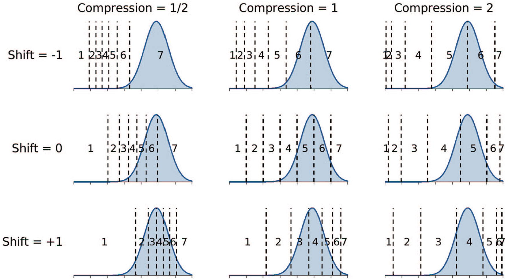
Demonstration of the linear-in-log-odds calibration model. The middle panel shows evenly spaced boundaries—corresponding to no shift or compression—that determine how a Gaussian distribution representing momentary judgments determines scale responses. The other panels show how these boundaries and response probabilities change when shift is changed to −1 and +1, and compression is changed to ½ and 2.

As the shift parameter becomes negative, the boundaries move down the scale, and the same momentary judgment leads to an increased probability of a higher rating. As shown in the center-top panel of Figure 3, when shift is −1 but compression is still 1, the most likely responses are only “6” and “7.” In contrast, as the shift parameter becomes positive, the boundaries move up the scale, and lower ratings become more likely.

If the compression parameter decreases below 1, the boundaries move closer together. The middle-left panel in Figure 3 shows the location of the boundaries when the compression is ½. These locations make end-point responses of “1” and “7” much more likely than responses in the middle of the scale. For the momentary judgment distribution in the example, this makes “7” the most likely response, followed by “6,” and so on. In contrast, as the compression parameter increases above one, the boundaries spread apart. This makes responses in the middle of the scale more likely and decreases the probability of end-point responses. The middle-right panel of Figure 3 shows that when compression is 2, responses of “4” and “5” are most likely.

Model Implementation

To formalize the linear-in-log-odds model, it is convenient to consider the momentary judgments being sampled on the unit interval. If there are $n$ possible scale responses, the evenly spaced boundaries fall at $k / n_{s}$ for $k = 1, \dots, n_{s} - 1$ . For a shift $α$ and a compression $β$ , these boundaries are transformed as

τ_{k} = \frac{\exp β {(k / n_{s})}^{α}}{\exp β {(k / n_{s})}^{α} + {(1 - k / n_{s})}^{α}},

(1)

with priors $α \sim G a u s s i a n (0, 1)$ and $β \sim Gaussian (0, 1)$ .

We modeled the momentary judgments as being sampled from a truncated Gaussian distribution⁴ with a mode $μ$ and a standard deviation $σ$ , so that

x \sim Gaussian (μ, 1 / σ^{2}) T (0, 1),

(2)

with priors m $\sim uniform (0, 1)$ and $σ \sim uniform (0, 1 / 2)$ .

The observed response is the censored measurement of $x$ according to the boundaries $τ$ , so that the observed response $y$ is given by

y = {\begin{array}{l} 1 & if x < τ_{1} \\ 2 & if τ_{1} \leq x < τ_{2} \\ \dots \\ k & if τ_{k - 1} \leq x < τ_{k} \\ \dots \\ n_{s} & if τ_{n_{s} - 1} \leq x . \end{array} .

(3)

To apply the linear-in-log-odds model to our experimental data, we assume that every question has its own truncated Gaussian distribution of momentary judgments. This distribution is the one that every participant samples from, regardless of the scale they use. We also assume that each of the five scales is characterized by its own shift and compression parameters that set boundaries. These boundaries are assumed to be the same for all participants and apply to all questions. Thus, the generative model of the observed ratings is that the participant samples a momentary judgment from the question distribution, and then applies the boundaries for the scale they were using for that question to produce their response.

We implemented this model as a graphical model in JAGS (Plummer, 2003). JAGS is software that provides a high-level scripting language for specifying models and automatically uses computational methods to conduct Bayesian inference. The JAGS script is available in the online Supplementary Material. The results we report are based on eight chains each containing 5,000 samples collected after 1,000 burn-in samples, and with no thinning of the chains. The $\hat{R}$ statistic (Brooks & Gelman, 1997) indicated good convergence, with all parameters having $\hat{R} < 1.005$ .

We conducted a posterior predictive check of the ability of the model to describe the observed data. The posterior predictive distribution is the pattern of response data generated by applying the model using the posterior distribution. It can be thought of as the model’s attempt to redescribe or “fit” the behavioral data. The correlation between the observed behavioral data—that is, the counts of how often a participant chose each response option for each scale and topic—and those produced by the model was 0.82 with a bootstrapped 95% confidence interval of [0.80, 0.84]. A scatter plot also showed that the absolute level of agreement between the data and model was good. Overall, the posterior predictive analysis provided evidence that the model accounts for the experimental data reasonably well.

Modeling Results

Boundary Inferences

Figure 4 summarizes the inferred posterior distribution of the shift and compression parameters for all five scales. The markers show the posterior means, and the error bars show 95% credible intervals for each parameter. It is clear that all the scales have a negative shift, which means higher responses on the scales are more likely. It is also clear that the compression is either near 1 or above 1, which means that the scale middle points are expanded resulting in less use of the end-points.

Figure 4.

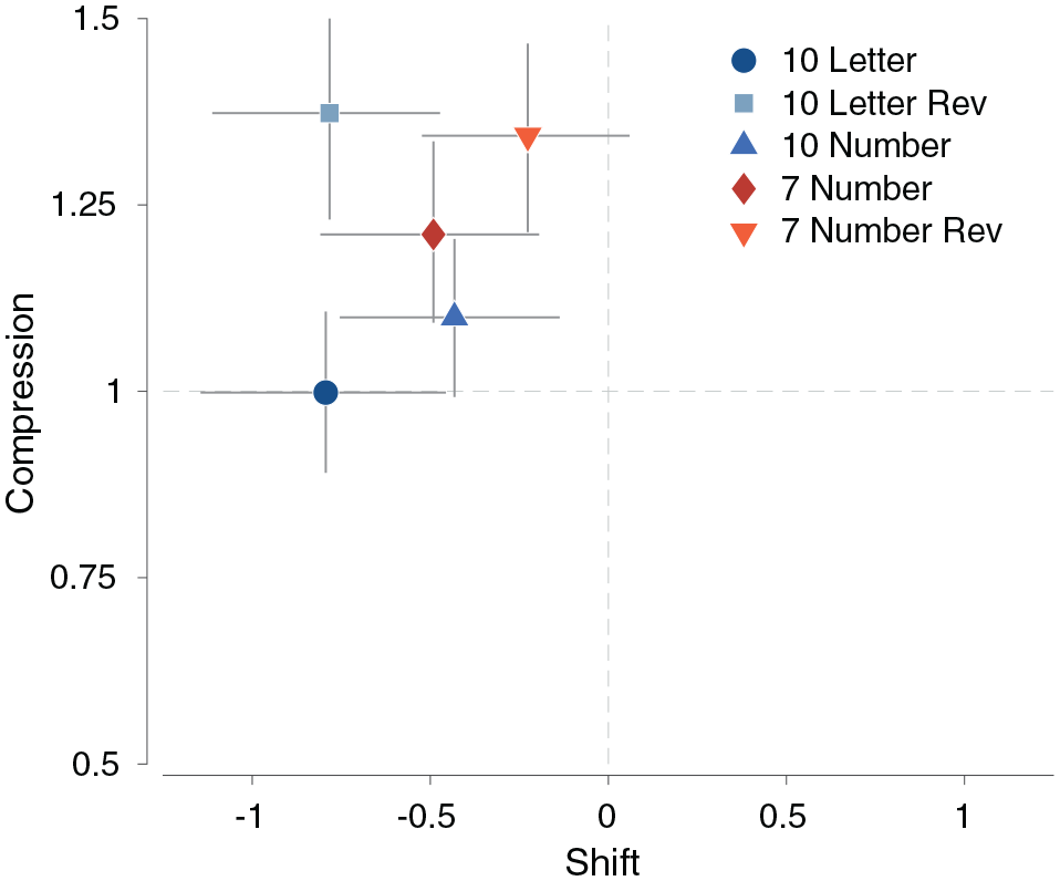
The joint posterior distributions of the shift and compression parameters for all five scales. The markers correspond to the posterior means, and the error bars show 95% credible intervals.

Beyond these broad commonalities, there are interpretable patterns of differences between the response scales. The 10-letter scales have the largest negative shift. This suggests that they lead to more positive rating responses. The two reversed scales have the largest compression values, indicating that they lead to reduced use of end-points. The combination of negative shift and high compression means that these scales especially promote the use of the positive middle points on the scale.

One perspective is that it is desirable for a response scale to have a shift of 0 and a compression of 1. This corresponds to evenly spaced boundaries and is represented by the origin in Figure 4. It is unclear which response scale is the best under this criterion, because some perform better with shift, while others perform better with compression.

Figure 5 summarizes the inferences about the boundaries for each of the five response scales. The boundaries shown correspond to the posterior means, and the error bars represent 95% credible intervals. The reversed scales were presented in the experiment from the highest to the lowest rating but are shown from the lowest to the highest for visual comparison. It is clear that the different response scales will often lead to the same momentary judgment causing different rating responses. For example, a momentary judgment that produces an “A” on the 10-letter scale is about equally likely to produce either an “A” or an “A−” on the reversed 10-letter scale, or a “10” or a “9” on the 10-number scale.

Figure 5.

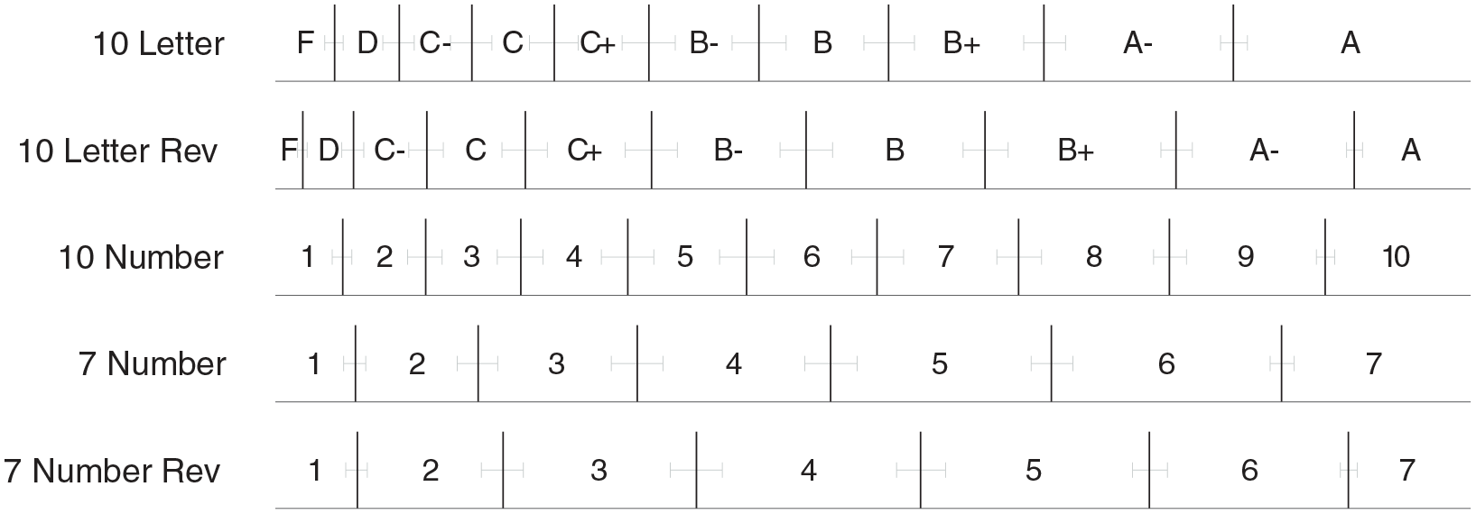
The inferred boundaries for each of the five response scales, partitioning the scale into the seven or 10 possible rating responses. The error bars show 95% credible intervals for each boundary. Reversed scales were presented in the experiment from the highest to the lowest rating, but are shown from the lowest to the highest for visual comparison.

The alignment of the boundaries in Figure 5 also provides some indication of how responses relate across different scales. The letter response “B−” is most likely to correspond to a “5,” or perhaps a “6,” on the 10-number scale. It is most likely to correspond to a “4,” however, on the 7-number scale.

Mapping Between Scales

Figure 6 demonstrates a more complete analysis of how responses on one scale map to responses on a different scale, according to the model. Intuitively, the inferred boundary shown in Figure 5 provides the information to map a response on one scale into possible responses on another scale. For example, a rating of 7 on the 7-number scale is most likely to map to a rating of 7 on the 7-number reverse, but there is some smaller probability that it will be a rating of 6. The mapping probabilities in Figure 6 are based on this logic, but incorporate the uncertainty about the boundaries.

Figure 6.

Probabilities of responses on one scale mapping to various possible responses on another response scale, according to the model-based analysis. In the left panel, the probabilities and shading show the probabilities of responses on the 7-number scale ( $y$ -axis) mapping to the responses on the reversed 7-number scale ( $x$ -axis). In the right panel, the probabilities and shading show the probabilities of responses on the 7-number scale ( $y$ -axis) mapping to the responses on the 10-letter scale ( $x$ -axis).

The left panel shows how responses on the 7-number scale are expected to map to responses on the reversed version of that scale. For example, a rating of “5” has a 41% probability of being a “4” on the reversed scale, and a 59% probability of staying at “5.” In general, as visually apparent from the shading, most of the high probabilities fall along the diagonal. The same rating is most likely to be produced, but there is usually some significant probability that the reverse scale leads to a rating that is one lower.

The right panel shows how responses on the 7-number scale are expected to map to responses on the 10-letter scale. For example, a rating of “4” on the number scale has a 37% probability of being a “B,” a 55% probability of being a “B−,” and an 8% probability of being a “C+.” The complete set of analysis showing how responses on any of the five scales maps to any other scale are provided in the online Supplementary Material.

Application to Comparing Real-World Evaluations

One potential application of the modeling results relates to the ability to map responses between scales. It is often the case that real-world evaluations are done using different scales, but it would be useful to be able to compare distributions of ratings on a common scale. The scale mapping probabilities presented in Figure 6 provide a way of making these sorts of comparisons. To this end, we collected some real-world evaluation data and conducted a “proof of concept” comparison of evaluation distributions originally collected on different scales.

EaterEvals Data

We collected instructor evaluations from the EEE+ EaterEvals repository⁵ of student evaluations of teaching provided by the University of California Irvine. At the time of collection, the repository included a large number of evaluations from 2016 to 2019. We considered evaluations of both lower-division and upper-division courses in the School of Biological Sciences, which has about 4,000 undergraduate students, and the School of Social Sciences, which has about 6,000 undergraduate students distributed across a number of majors.

In particular, we scraped response data from 636 courses in the biological sciences major, 71 courses in the psychology major, 79 courses in the social sciences major, and 87 courses in the sociology major. Summer courses were excluded from data analysis because of the uncertainty in the student population, the use of a different scale than traditionally used in each department, and the difference in course length. We also excluded evaluations with fewer than 10 responses or less than 20% of the students providing evaluations. Subject to those exclusions, the class evaluations we used represented all the available data in the repository at the time of collection in Fall 2019.

Demonstration of Scale Mapping

We used the EEE+ EaterEvals data to demonstrate how ratings for the overall value of course and overall value of instructor evaluation questions for psychology, social science, and sociology majors could be affected if the department used a 10-letter scale, rather than the currently used 7-number scale scale. In total, we included about 13,000 assessments for 247 psychology, sociology, and social science classes made using a 7-number scale and about 53,000 assessments for 636 biology classes made using a 10-letter scale.

Figure 7 shows the scale mapping demonstration. The left panel shows ratings made when using the current 7-number scale. The middle panel shows ratings made within the biological sciences department using a 10-letter scale. The right panel shows the mapping of ratings from the 7-number scale to their equivalent distribution when using a 10-letter scale. An interesting result is that the overall distribution of 7-number ratings becomes much steeper and declines more rapidly when mapped to the 10-letter scale. In particular, the predicted use of the end-point “A” response is relatively greater than the proportion of the end-point “7” responses in the evaluations that were actually collected.

Figure 7.

An example of mapping from one scale to another. The left panels show the distribution ratings made using a 7-number scale for psychology, sociology, and social science classes. The middle panels show the distribution of grades for biology classes made using a 10-letter scale. The right panel shows both distributions on the same 10-letter scale, with the number scale grades mapped to the letter scale. The top row corresponds to the overall evaluation items for the instructor, and the bottom row corresponds to the overall evaluation items for the course.

Discussion

Our goal was to examine how scale properties affect student evaluation of teaching. To study this, we conducted a controlled experiment that varied the properties of scales used to evaluate instructor and course material. We then used a linear-in-log-odds model with two parameters, shift and compression, to examine the impact of scale properties on ratings.

In general, the participants exhibited an acquiescence bias (van Vaerenbergh & Thomas, 2013), meaning that the student ratings of instructor and course material were positive, on average, regardless of the scale used. This finding was most pronounced for the letter scales when compared with number scales. The 10-letter and 10-letter reverse scales exhibited the most extreme shift score, meaning that average ratings were the highest when using these scales. While the number scales still had a negative shift, meaning that students tended to use positive scale points, it was not as extreme as for the letter scales.

The participants also showed a reduced tendency to use the end-points of the scales, and this finding was most pronounced for the reversed scales. The 10-letter reverse and 7-number reverse scales exhibited the greatest compression, meaning that participants used the end-points less often than the middle points. Participants used the end-points most often when evaluating instructor and course material using the 10-letter scale compared with the other scales.

Scales presented in their normal order had higher average ratings from the students when compared with the reverse-ordered scales. Following Hartley and Betts (2010), we observed students giving instructor and course material higher ratings when using the 10-letter scale, with positive scale points on the left-hand side, compared with the 10-letter reverse scale. However, we did not observe this effect with the number scales. Students gave higher average ratings when using the 7-number scale, which had positive scale points on the right-hand side, compared with the 7-number reverse scale, which had positive scale points on the left-hand side.

The difference in scale labeling between letters and numbers had a clear effect on ratings of instructor and course material. As shown through the $t$ -test analysis of average evaluation scores, as well through the model-based analysis, students tend to give higher ratings when using letter scales compared with numerical scales. The 10-letter scale and the 10-letter reverse scale had the highest average ratings. Our study is the first that we are aware of to compare letter and numerical scales. What makes letter scales fundamentally different from numerical scales is not well understood and should be further investigated. It is possible that students conflate their use of letter scales with their prior experiences being graded and grade inflation. This notion of “grade leniency” and its impact on student evaluations of teaching is discussed by Stroebe (2016).

Finally, when applying our model to real-world evaluation data, we observed how scale design may affect instructor and course evaluations. Our model-based approach allowed us to map each scale onto the others. This allowed us to predict what distribution of evaluations a class would have provided if they had been given a different scale. Previous work on scale linkage has focused on predicting, aligning, and equating various tests outcomes, such as the Scholastic Assessment Test (Dorans et al., 2007). These methods allow for outcomes on various tests to be mapped to one common scale (Reardon et al., 2021). As far as we are aware, no previous studies have modeled and mapped data from different evaluation scales to their equivalent on another scale.

We think this collection of findings and the practical applications demonstrates the merits of our model-based approach to analysis and our use of Bayesian statistical methods. The combination of a cognitive model and Bayesian methods allowed for inferences about latent boundaries for comparing scales and for the examination of scale effects in terms of psychologically meaningful concepts of shift and compression. The applied demonstration, in which we mapped responses between scales, would not be possible without a model of responding that includes latent boundaries, and requires Bayesian methods to map the response probabilities in a way that is sensitive to the uncertainty about the locations of the boundaries.

An important limitation relates to the ecological validity of the task. Our methodological approach allows for a careful study of scale use, but is more limited in its ability to be generalized to student evaluations of teaching in the real world. Having participants read a transcript of a 5-minute TED-Ed video is not equivalent to attending a lecture-based course. While prior studies have used similar experimental materials to examine student evaluations of teaching and bias (Rivera & Tilcsik, 2019), we recognize the limitations of the transcript stimuli we used. The only way to address this weakness is through some form of field experiment in which, for example, a real-world course evaluation is manipulated so that different students use different scales for evaluation. The results from an experiment like this would provide a strong test of our modeling methods and preliminary conclusions.

Another potential limitation of our controlled experiment concerns our study population. All the participants were undergraduate students at the University of California Irvine. It would have been ideal to have student participants from different gender, racial, and ethnic backgrounds. On the other hand, our study population does provide a close approximation of the students represented in the EEE+ EaterEvals data set.

Future research should explore the impacts of scale design when evaluating instructors of varying genders, races, or ethnicities. Prior research demonstrates such characteristics affect student ratings. Female instructors are repeatedly rated lower than male instructors, especially in math-related or high-status fields, and this finding has been observed in both quasi-natural experiments and controlled experiments that only varied in gender of the professor (Arbuckle & Williams, 2003; Fisher et al., 2019; Mengel et al., 2019; Mitchell & Martin, 2018; Rivera & Tilcsik, 2019). In terms of ethnicity, White professors are often rated higher than their non-White counterparts (Bavishi et al., 2010; Chávez & Mitchell, 2020).

Another potential direction of future research could explore the impact of varying the wording of scale labels in addition to varying the number of points on the scale. Prior studies suggest that scale labels affect people’s responses. For example, using harsher end-point labels results in less variability of usage of the scale points (Weijters et al., 2013; Wyatt & Meyers, 1987). In the present study, we used the same worded labels for our numeric scales. Further research can manipulate scale labeling in conjunction with the number of points on the scale to observe how these scale properties may affect responses.

In conclusion, our study has implications for scale design, comparing ratings across scales, and using scales for administrative decisions. Understanding how scales affect student evaluations of teaching is an important step for recognizing and correcting scale-induced effects.

Footnotes

Acknowledgements

We thank Paul de Boeck, members of the Bayesian Cognitive Modeling Lab at the University of California Irvine, and three anonymous reviewers for helpful comments. An Open Science Framework repository and an Inter-university Consortium for Political and Social Research project with experimental materials, data, and model code are available at https://osf.io/47jys/ and , respectively. This research was supported by University of California Irvine UROP and SURP funding to KC.

ORCID iDs

Karyssa A. Courey

Michael D. Lee

Notes

Authors

KARYSSA A. COUREY is a psychology graduate from the University of California Irvine and a current graduate student at the Rice University. Her research interests include evaluation bias, individual differences, decision making, and Bayesian methods with a focus on enhancing diversity in the workplace.

MICHAEL D. LEE is a professor of cognitive sciences at the University of California Irvine. His research interests are in models of cognition, including representation, memory, learning, and decision making, with a special focus on individual differences and Bayesian methods.

References

Anders

Batchelder

(2015). Cultural consensus theory for the ordinal data case. Psychometrika, 80, 151–181. https://doi.org/10.1007/s11336-013-9382-9

Andrich

(1978). A rating formulation for ordered response categories. Psychometrika, 43, 561–573. https://doi.org/10.1007/BF02293814

Arbuckle

Williams

B. D.

(2003). Students’ perceptions of expressiveness: Age and gender effects on teacher evaluations. Sex Roles, 49, 507–516. https://doi.org/10.1023/A:1025832707002

Bavishi

Madera

J. M.

Hebl

M. R.

(2010). The effect of professor ethnicity and gender on student evaluations: Judged before met. Journal of Diversity in Higher Education, 3(4), 245–256. https://doi.org/10.1037/a0020763

Bazán

J. L.

Bolfarine

Branco

M. D.

(2006). A skew item response model. Bayesian Analysis, 1(4), 861–892. https://doi.org/10.1214/06-BA128

Bolfarine

Bazan

J. L.

(2010). Bayesian estimation of the logistic positive exponent IRT model. Journal of Educational and Behavioral Statistics, 35(6), 693–713. https://doi.org/10.3102/1076998610375834

Bolt

D. M.

Lee

Wollack

Eckerly

Sowles

(2018). Application of asymmetric IRT modeling to discrete-option multiple-choice test items. Frontiers in Psychology, 9, Article 2175. https://doi.org/10.3389/fpsyg.2018.02175

Brooks

S. P.

Gelman

(1997). General methods for monitoring convergence of iterative simulations. Journal of Computational and Graphical Statistics, 7(4), 434–455. https://doi.org/10.1080/10618600.1998.10474787

Brown

(2000). What issues affect Likert-scale questionnaire formats? JALT Testing & Evaluation SIG, 4(1), 27–30. https://doi.org/10.1177/0049124108330004

10.

Chan

J. C.

(1999). Response-order effects in Likert-type scales. Educational and Psychological Measurement, 51(3), 531–540. https://doi.org/10.1177/0013164491513002

11.

Chávez

Mitchell

K. M.

(2020). Exploring bias in student evaluations: Gender, race, and ethnicity. PS: Political Science & Politics, 53, 270–274. https://doi.org/10.1017/S1049096519001744

12.

Christian

L. M.

Parsons

N. L.

Dillman

D. A.

(2009). Designing scalar questions for web surveys. Sociological Methods & Research, 37(3), 393–425. https://doi.org/10.1177/0049124108330004

13.

Chyung

S. Y.

Kennedy

Campbell

(2018). Evidence-based survey design: The use of ascending or descending order of Likert-type response options. Performance Improvement, 57(9), 9–16. https://doi.org/10.1002/pfi.21800

14.

Colman

A. M.

Norris

C. E.

Preston

C. C.

(1997). Comparing rating scales of different lengths: Equivalence of scores from 5-point and 7-point scales. Psychological Reports, 80(2), 355–362. https://doi.org/10.2466/pr0.1997.80.2.355

15.

Cox

E. P.

(1980). The optimal number of response alternatives for a scale: A review. Journal of Marketing Research, 17(4), 407–422. https://doi.org/10.2307/3150495

16.

Croasmun

J. T.

Ostrom

(2011). Using Likert-type scales in the social sciences. Journal of Adult Education, 40(1), 19–22.

17.

Dawes

(2008). Do data characteristics change according to the number of scale points used? An experiment using 5-point, 7-point and 10-point scales. International Journal of Market Research, 50(1), 61–104. https://doi.org/10.1177/147078530805000106

18.

De Boeck

Wilson

. (Eds.). (2004). Explanatory item response models. Springer. https://doi.org/10.1007/978-1-4757-3990-9

19.

Diamantopoulos

(2006). The error term in formative measurement models: interpretation and modeling implications. Journal of Modelling in Management, 1(1), 7–17. https://doi.org/10.1108/17465660610667775

20.

Dorans

N. J.

Pommerich

Holland

P. W.

(2007). Linking and aligning scores and scales. Springer Science+Business Media. https://doi.org/10.1007/978-0-387-49771-6

21.

Etz

Vandekerckhove

(2018). Introduction to Bayesian inference for psychology. Psychonomic Bulletin & Review, 25, 5–34. https://doi.org/10.3758/s13423-017-1262-3

22.

Falk

C. F.

(2020). Estimation of response styles using the multidimensional nominal response model: A tutorial and comparison with sum scores. Frontiers in Psychology, 11, Article 72. https://doi.org/10.3389/fpsyg.2020.00072

23.

Fisher

A. N.

Stinson

D. A.

Kalajdzic

(2019). Unpacking backlash: Individual and contextual moderators of bias against female professors. Basic and Applied Social Psychology, 41(5), 305–325. https://doi.org/10.1080/01973533.2019.1652178

24.

Fox

C. R.

Tversky

(1995). Ambiguity aversion and comparative ignorance. Quarterly Journal of Economics, 110(3), 585–603. https://doi.org/10.2307/2946693

25.

Givon

M. M.

Shapira

(1984). Response to rating scales: A theoretical model and its application to the number of categories problem. Journal of Marketing Research, 21(4), 410–419. https://doi.org/10.1177/002224378402100406

26.

Gonzalez

(1999). On the shape of the probability weighting function. Cognitive Psychology, 38(1), 129–166. https://doi.org/10.1006/cogp.1998.0710

27.

Hartley

Betts

L. R.

(2010). Four layouts and a finding: The effects of changes in the order of the verbal labels and numerical values on Likert-type scales. International Journal of Social Research Methodology, 13(1), 17–27. https://doi.org/10.1080/13645570802648077

28.

InfoPlease. (2017). The top ten: Most common last names in the U.S. https://www.infoplease.com/us/population/most-common-last-names-us

29.

JASP Team. (2020). JASP (Version 0.14.1) [Computer software]. https://jasp-stats.org/

30.

Jenkins

G. D.

Taber

T. D.

(1977). A Monte Carlo study of factors affecting three indices of composite scale reliability. Journal of Applied Psychology, 62(4), 392–398. https://doi.org/10.1037/0021-9010.62.4.392

31.

Jin

K.-Y.

Wang

W.-C.

(2014). Generalized IRT models for extreme response style. Educational and Psychological Measurement, 74(1), 116–138. https://doi.org/10.1177/0013164413498876

32.

Johnson

T. R.

Bolt

D. M.

(2010). On the use of factor-analytic multinomial logit item response models to account for individual differences in response style. Journal of Educational and Behavioral Statistics, 35(1), 92–114. https://doi.org/10.3102/1076998609340529

33.

Kass

R. E.

Raftery

A. E.

(1995). Bayes factors. Journal of the American Statistical Association, 90(430), 773–795. https://doi.org/10.1080/01621459.1995.10476572

34.

Krosnick

J. A.

(2018). Questionnaire design. In Vannette

D. L.

Krosnick

J. A.

(Eds.), The Palgrave handbook of survey research (pp. 439–455). Palgrave Macmillan. https://doi.org/10.1007/978-3-319-54395-6_53

35.

Krosnick

J. A.

Holbrook

A. L.

Berent

M. K.

Carson

R. T.

Michael Hanemann

Kopp

R. J.

Mitchell

R. C.

Presser

Ruud

P. A.

Smith

V. K.

Moody

W. R.

Green

M. C.

Conaway

(2002). The impact of “no opinion” response options on data quality: Non-attitude reduction or an invitation to satisfice? Public Opinion Quarterly, 66(3), 371–403. https://doi.org/10.1086/341394

36.

Kulas

J. T.

Stachowski

A. A.

(2009). Middle category endorsement in odd-numbered Likert response scales: Associated item characteristics, cognitive demands, and preferred meanings. Journal of Research in Personality, 43(3), 489–493. https://doi.org/10.1016/j.jrp.2008.12.005

37.

Kulas

J. T.

Stachowski

A. A.

Haynes

B. A.

(2008). Middle response functioning in Likertresponses to personality items. Journal of Business and Psychology, 22, 251–259. https://doi.org/10.1007/s10869-008-9064-2

38.

Leung

S.-O.

(2011). A comparison of psychometric properties and normality in 4-, 5-, 6-, and 11-point Likert scales. Journal of Social Service Research, 37(4), 412–421. https://doi.org/10.1080/01488376.2011.580697

39.

Lissitz

R. W.

Green

S. B.

(1975). Effect of the number of scale points on reliability: A Monte Carlo approach. Journal of Applied Psychology, 60(1), 10–13. https://doi.org/10.1037/h0076268

40.

Marsh

H. W.

Roche

L. A.

(1997). Making students’ evaluations of teaching effectiveness effective: The central issues of validity, bias, and utility. American Psychologist, 52(11), 1187–1197. https://doi.org/10.1037//0003-066X.52.11.1187

41.

Matzke

Boehm

Vandekerckhove

(2018). Bayesian inference for psychology, part iii: Parameter estimation in nonstandard models. Psychonomic Bulletin & Review, 25(1), 77–101. https://doi.org/10.3758/s13423-017-1394-5

42.

Mengel

Sauermann

Zölitz

(2019). Gender bias in teaching evaluations. Journal of the European Economic Association, 17(2), 535–566. https://doi.org/10.1093/jeea/jvx057

43.

Mitchell

K. M. W.

Martin

(2018). Gender bias in student evaluations. PS: Political Science & Politics, 51(3), 648–652. https://doi.org/10.1017/S104909651800001X

44.

Moors

Kieruj

N. D.

Vermunt

J. K.

(2014). The effect of labeling and numbering of response scales on the likelihood of response bias. Sociological Methodology, 44(1), 369–399. https://doi.org/10.1177/0081175013516114

45.

Nicholls

M. E.

Orr

C. A.

Okubo

Loftus

(2006). Satisfaction guaranteed: The effect of spatial biases on responses to Likert scales. Psychological Science, 17(12), 1027–1028. https://doi.org/10.1111/j.1467-9280.2006.01822.x

46.

O’Muircheartaigh

C. A.

Krosnick

J. A.

Helic

(2001). Middle alternatives, acquiescence, and the quality of questionnaire data (Working Paper 0103). Harris School of Public Policy Studies, University of Chicago. https://ideas.repec.org/p/har/wpaper/0103.html

47.

Otto

Sanford

D. A.

Ross

D. N.

(2008). Does ratemyprofessor.com really rate my professor? Assessment & Evaluation in Higher Education, 33, 355–368. https://doi.org/10.1080/02602930701293405

48.

Paulhus

D. L.

(1991). Measurement and control of response bias. In Robinson

J. P.

Shaver

P. R.

Wrightsman

L. S.

(Eds.), Measures of personality and social psychological attitudes (pp. 17–59). Academic Press. https://doi.org/10.1016/B978-0-12-590241-0.50006-X

49.

Plummer

(2003). JAGS: A program for analysis of Bayesian graphical models using Gibbs sampling. In Hornik

Leisch

Zeileis

(Eds.), Proceedings of the 3rd International Workshop on Distributed Statistical Computing (DSC 2003). https://www.r-project.org/conferences/DSC-2003/Proceedings/Plummer.pdf

50.

Reardon

S. F.

Kalogrides

A. D.

(2021). Validation methods for aggregate-level test scale linking: A case study mapping school district test score distributions to a common scale. Journal of Educational and Behavioral Statistics, 46(2), 138–167. https://doi.org/10.3102/1076998619874089

51.

Rivera

L. A.

Tilcsik

(2019). Scaling down inequality: Rating scales, gender bias, and the architecture of evaluation. American Sociological Review, 84(2), 248–274. https://doi.org/10.1177/0003122419833601

52.

Samejima

(2000). Logistic positive exponent family of models: Virtue of asymmetric item characteristic curves. Psychometrika, 65, 319–335. https://doi.org/10.1007/BF02296149

53.

Selker

van den Bergh

Criss

A. H.

Wagenmakers

E.-J.

(2019). Parsimonious estimation of signal detection models from confidence ratings. Behavior Research Methods, 51(5), 1953–1967. https://psycnet.apa.org/doi/10.3758/s13428-019-01231-3

54.

Social Security Administration. (2019). Top names of the 1960s. https://www.ssa.gov/oact/babynames/decades/names1960s.html

55.

Stroebe

(2016). Why good teaching evaluations may reward bad teaching: On grade inflation and other unintended consequences of student evaluations. Perspectives on Psychological Science, 11(6), 800–816. https://doi.org/10.1177/1745691616650284

56.

Thissen

Cai

Bock

R. D.

(2010). The nominal categories item response model. In Nering

M. L.

Ostini

(Eds.), Handbook of polytomous item response theory models (pp. 43–76). Taylor & Francis.

57.

Thurstone

L. L.

(1927). A law of comparative judgement. Psychological Review, 34(4), 273–286. https://doi.org/10.1037/h0070288

58.

Vandekerckhove

Rouder

J. N.

Kruschke

J. K.

(2018). Editorial: Bayesian methods for advancing psychological science. Psychonomic Bulletin & Review, 25, 1–4. https://doi.org/10.3758/s13423-018-1443-8

59.

van der Linden

W. J.

Hambleton

R. K

. (2013). Handbook of modern item response theory. Springer Science & Business Media.

60.

van Vaerenbergh

Thomas

T. D

. (2013). Response styles in survey research: A literature review of antecedents, consequences, and remedies. International Journal of Public Opinion Research, 25(2), 195–217. https://doi.org/10.1093/ijpor/eds021

61.

Wagenmakers

E.-J.

Marsman

Jamil

Verhagen

Love

Selker

Gronau

Q. F.

Šmíra

Epskamp

Matzke

Rouder

J. N.

Morey

R. D.

(2018). Bayesian inference for psychology. Part I: Theoretical advantages and practical ramifications. Psychonomic Bulletin & Review, 25, 35–57. https://doi.org/10.3758/s13423-017-1343-3

62.

Wagenmakers

E.-J.

Morey

R. D.

Lee

M. D.

(2016). Bayesian benefits for the pragmatic researcher. Current Directions in Psychological Science, 25(3), 169–176. https://doi.org/10.1177/0963721416643289

63.

Weijters

Geuens

Baumgartner

(2013). The effect of familiarity with the response category labels on item response to Likert scales. Journal of Consumer Research, 40(2), 368–381. https://doi.org/10.1037/a0018721

64.

Weijters

Geuens

Schillewaert

(2010). The stability of individual response styles. Psychological Methods, 15(1), 96–110. https://doi.org/10.1086/670394

65.

Weng

L.-J.

Cheng

C.-P.

(2000). Effects of response order on Likert-type scales. Educational and Psychological Measurement, 60(6), 908–924. https://doi.org/10.1177/00131640021970989

66.

Wetzel

Lüdtke

Zettler

Böhnke

J. R.

(2016). The stability of extreme response style and acquiescence over 8 years. Assessment, 23(3), 279–291. https://doi.org/10.1177/1073191115583714

67.

Willits

F. K.

Theodori

G. L.

Luloff

(2016). Another look at Likert scales. Journal of Rural Social Sciences, 31(3), Article 6. https://egrove.olemiss.edu/cgi/viewcontent.cgi?article=1073&context=jrss

68.

Leung

S.-O.

(2017). Can Likert scales be treated as interval scales? A simulation study. Journal of Social Service Research, 43(4), 527–532. https://doi.org/10.1080/01488376.2017.1329775

69.

Wyatt

R. C.

Meyers

L. S.

(1987). Psychometric properties of four 5-point Likert type response scales. Educational and Psychological Measurement, 47(1), 27–35. https://doi.org/10.1177/0013164487471003

A Model-Based Examination of Scale Effects in Student Evaluations of Teaching

Abstract

Keywords

Empirical Evidence for Examining Scale Properties

Effects of Scale Properties on Evaluations

Methods for Evaluating Scale Properties

Current Aims and Approach

Method

Participants

Procedure

Basic Results

Model-Based Analysis

Model Intuitions

Model Implementation

Modeling Results

Boundary Inferences

Mapping Between Scales

Application to Comparing Real-World Evaluations

EaterEvals Data

Demonstration of Scale Mapping

Discussion

Footnotes

Acknowledgements

ORCID iDs

Notes

Authors

References