
Abstract
Homestead exemptions for senior and disabled homeowners disproportionally erode rural tax bases but may still stimulate local educational spending. This article examines one such exemption in Kentucky. Two-stage generalized method of moments is used to estimate the demand for local education spending, then spending in the absence of the exemption is simulated to estimate effects on school district expenditure and academic performance. We combine Census and National Center of Education Statistics data with detailed exemption and academic performance data from Kentucky’s Departments of Revenue and Education into a panel spanning 1999–2013. Results suggest the exemption provides relatively generous tax relief without increasing resource and academic achievement gaps between rural and nonrural districts. This is largely attributable to Kentucky’s strong school finance equalization effort. Our findings can help states with a similarly targeted exemption consider such impacts in relation to their own demography and funding systems.
Keywords
Approximately 20 states offer homestead exemptions to seniors and/or those with a disability without reimbursing local governments for lost revenue (Duncombe & Yinger, 2001; Lincoln Institute of Land Policy and George Washington Institute of Public Policy, 2019). Among them, disability and senior household rates are five and seven percentage points greater in rural counties, respectively (U.S. Census Bureau, 2017a, 2017b). Such differences suggest homestead exemptions that target seniors or disabled people may disproportionately erode tax bases in rural school districts, leading to disparities in educational resources and student achievement. However, most studies find that educational spending rises in response to property tax exemptions due to a corresponding decline in the median voter’s share of the cost (Addonizio, 1991; Brien & Sjoquist, 2014; Eom et al., 2014; Fisher & Rasche, 1984; Rockoff, 2010). Variation in exemption features and school equalization effort warrants additional research in order to understand the extent to which such exemptions impact rural education finance. This article examines the effects of a homestead exemption for seniors and disabled people on school district expenditure and academic performance in Kentucky.
Kentucky offers valuable context to this line of inquiry in several respects beyond its targeted exemption. Almost all states have multiple exemption programs with overlapping eligibility and different levels of relief. Kentucky is one of only two states with a single exemption program, allowing us to examine its impact in isolation. Moreover, the exemption does not include local options that cause relief to vary by county, it is not means tested, and relief is capped at a flat dollar amount. Relative to states with similarly targeted exemptions, Kentucky’s disparity in senior and disability rates between rural and nonrural counties is about average, but its exemption is among the most generous in terms of the percent of property tax revenue lost. Last, Kentucky outranks most states with regard to its school finance equalization effort (Hightower et al., 2010; U.S. Government Accountability Office, 1998). Since state aid is inversely related to taxable property wealth, we examine the efficacy of Kentucky’s equalization efforts at offsetting any interdistrict disparity caused by its exemption.
We use panel data from 1999 to 2013 to estimate a demand function for local education spending in the presence of Kentucky’s homestead exemption, then simulate local spending in the absence of the exemption. We find that the price elasticity of demand associated with the exemption is modest. This is perhaps due to the low salience of the exemption among most taxpayers. Due to the low magnitude of the price elasticity, the price effect of the exemption on expenditure is negligible in the vast majority of areas where the fraction of property wealth that is exemptible is small, and it is almost completely offset by the state aid effect. In areas where the exemption claims a large fraction of property wealth, but the median voter is not likely to claim the exemption, the median voter’s tax price is significantly higher, but the low-price elasticity combined with the offsetting increase in state aid lead to a modest net gain in expenditure. In districts where it is likely that the median voter is a claimant, the exemption greatly reduces the tax price of the median voter and increases the amount of state aid, but the price reduction reduces the benefit that the median voter derives from state aid to a large enough degree that the net increase in expenditure is modest.
The largest expenditure impacts that we observe lead to increases in standardized test performance of about 0.001 standard deviations. These are weak effect sizes relative to many of the education interventions that have been studied by researchers (Yeh, 2010). The extent to which the resulting property tax increases crowd out the tax relief provided to senior and disabled homeowners ranges from −0.55% to −12%. Overall, the results suggest that Kentucky’s homestead exemption provides relatively generous tax relief to the disabled and seniors without increasing the resource and academic achievement gaps between rural and nonrural districts.
The article is organized as follows. The next section provides relevant background information and the conceptual framework. The subsequent section describes the empirical strategy and data. Estimation results are presented in the penultimate section, as well as simulations of the impacts of the homestead exemption on spending, property tax rates, and academic performance. We conclude with some discussion of the practical policy implications of the findings and possibly fruitful avenues for future research.
Background and Conceptual Framework
Since 1972, Kentucky state government has made fully disabled homeowners as well as those aged 65 years or older eligible for a sizable homestead exemption. The exemption amount is recalculated every 2 years to adjust for inflation. In 2013, the exemption was equal to $36,000, which is equal to about 32% of the median home value in the state. For the average county, the homestead exemption wiped away about 10% of potential assessed value. There is considerable variation among counties. As Figure 1 shows, rural counties experience substantially higher levels of property tax base erosion due to the homestead exemption. In 2013, all the counties in the top decile of the state distribution of exemption rates were located in the Appalachian region. Among these districts, the average percentage of gross value lost to exemptions was 21%. About 43% of the exempted property value of these counties belonged to disabled homeowners.

Percent property base erosion due to homestead exemption in Kentucky counties, FY 2018.
How have these local revenue base losses affected school district expenditures? Calculating the property tax revenue that is forgone due to the homestead exemption based on current property tax rates would not provide an accurate estimate. That is because districts can levy higher property tax rates to offset base reductions. Additionally, the amount of property value exempted increases the amount of state aid received by districts, since the amount of aid received is inversely related to taxable property value. Thus, it is necessary to utilize a demand function for local education spending and model the role played by the homestead exemption.
The public finance literature on the demand for state and local public services has focused on variables that potentially have price and income effects on the demand of these services by voters. The conceptual framework that guides these studies typically features a government that chooses expenditure for each category to maximize the expected votes that it receives in the next election. Voters derive utility from public spending and disutility from the full income loss, which includes deadweight losses from taxation. Policy makers expect voters to support the fiscal platform that gives them the greatest net utility. Bergstrom and Goodman (1973), Zimmerman (1983), and Gade and Adkins (1990), among many others, posit that each voter’s preferred fiscal platform is proportional to their income. 1 By the median voter theorem, the politically optimal fiscal platform is that which is preferred by the voter with the median income.
By specifying a utility function for the median voter and a budget constraint for both the voter and the government, the analyst can solve for an explicit demand function for public services. When the policy outcome of interest is expenditure, it is customary to assume a constant elasticity demand function of the following form (Duncombe, 1996):
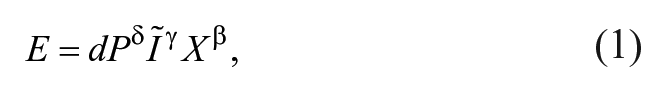
where E denotes education expenditure per pupil, d is a constant that represents time-invariant idiosyncrasies that influence the median voter’s preferences, P denotes the median voter’s price for educational services,
In a context in which the government taxes assessed market value in its entirety, and there are no exemptions or tax credits, the price term (P) is given by

where V is the median home value in the school district,
The existence of exemptions or credits can alter the tax price. Research on Michigan’s circuit breaker conducted by Fisher and Rasche (1984) and Addonizio (1991) find that it reduced the tax prices faced by communities and stimulated education spending. Previous research on homestead exemptions has explored cases in which most or all homeowners were eligible for the exemption and state government reimbursed districts for the lost property tax revenue. Brien and Sjoquist (2014) examine a state-funded property tax exemption program in Georgia and find that it functions like a matching grant and lowers the tax price of local education spending for the median voter that increases local property tax revenue. Looking at the state-funded STAR (School Tax Relief) property tax exemption in New York, Rockoff (2010) and Eom et al. (2014) find that it reduced the median voter’s tax price and placed significant upward pressure on school district expenditure. In states such as Illinois where the homestead exemption is available to most homeowners and is not offset by state transfers, the median voter’s tax price is lower only if the median voter’s home value net of the exemption is less than assessed value per pupil (Brien & Sjoquist, 2014).
In Kentucky, however, only senior and disabled homeowners are eligible for an exemption, and the property tax revenue lost is not reimbursed by the state. Thus, if the median voter is not senior or disabled, the Kentucky homestead exemption raises the median voter’s tax price by reducing district aggregate assessed value per-pupil while leaving the median voter’s assessed home value unchanged. If the median voter is senior or disabled, and claims the exemption, their taxable property is reduced by the exemption amount. We rewrite the formula for P to reflect these effects:
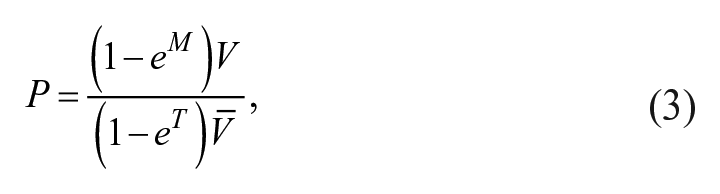
where
If the median voter is senior or disabled, then the numerator of Equation 3,
The price effect is not the only channel through which the Kentucky homestead exemption affects demand for education spending. Because the Kentucky aid formula awards more aid to districts with relatively low levels of per pupil taxable property value, the homestead exemption increases state aid per pupil. State aid in Kentucky consists of the SEEK (Support Education Excellence in Kentucky) program, which is a minimum foundation aid plan, and the Tier 1 program, which is a close-ended matching grant. The amount of state SEEK aid received by a district is given by

where M is the state minimum level of expenditure per pupil,
The other major component of state aid is the Tier 1 matching grant. For districts with per pupil property wealth less than 1.5 times the statewide average district per pupil property value, the Tier 1 program provides additional state funding. For local tax rates above the minimum that localities must levy to receive SEEK funds, Tier 1 aid tops up local funds to the level that would be raised if the local rate were applied to 1.5 times the statewide average per-pupil assessed value. In other words, local effort in the Tier 1 range is equalized at 150% of the average base. The Tier 1 formula allows districts to generate additional state and local funds up to 15% of their adjusted SEEK base guarantee. Thus, it is a close-ended matching grant. When a district reaches the maximum, the Tier 1 grant is essentially a lump-sum grant. However, the funding amount continues to depend on a district’s assessed property value relative to the equalization level. Thus, use of the exemption by a district’s residents leads to additional Tier 1 aid. All the Tier 1–eligible districts in our panel are at the maximum level. Thus, we treat Tier 1 aid as lump-sum aid in the analysis.
State aid enters the median voter’s demand function as part of their “augmented income,” which is the sum of private income and a portion of per-pupil state aid:

where I denotes private income, A is state aid per pupil, and f is a flypaper effect. It is unlikely that the elasticity of state aid is the same as the private income elasticity. To facilitate the separate estimation of the income and aid elasticities in the demand analysis, we rewrite the equation for augmented income:

The flypaper effect f influences the value of state aid to the median voter since aid is not received directly by households but by the government. Though a portion of the aid is typically passed forward to residents in the form of tax cuts, the proportion that is spent on primary education tends to be greater than what would be spent from an equivalent increase in private income, which is the flypaper effect (Eom et al., 2014; Oates, 1999). The value of state aid to the median voter is also mediated by their tax price since state aid substitutes for local tax dollars to some degree. This substitutive effect of state aid is more (less) valuable to the median voter the higher (lower) is their tax price. In districts in which the median voter is not eligible for the exemption, tax base erosion due to the exemption increases their tax price, which places downward pressure on their demand for education spending. That downward pressure is offset by an income effect from additional state aid that is magnified by the higher tax price. In other words, district-wide use of the exemption makes a non–claimant median voter’s demand for education spending more sensitive to the additional state aid brought about by the exemption. In districts where the median voter is an exemption claimant, the exemption lowers the tax price that leads to a positive price effect on demand, but it has conflicting impacts on the median voter’s aid share. Like all other districts, a district in which the median voter is a claimant receives additional state aid per-pupil. However, the price decrease reduces the median voter’s share of state aid and could conceivably be large enough to overpower the impact of the aid increase and lead to a negative income effect, which offsets the positive price effect.
At this point, we have demonstrated that the homestead exemption potentially has price and income effects on school district expenditure. In the following section, we estimate a demand function for per-pupil expenditure for Kentucky school districts. We then gauge the impact of the homestead exemption by calculating the differences in the median voter’s tax and state aid shares that are attributable to the exemption. We then combine these differences with the relevant elasticities from the demand equation to arrive at the net effects on per-pupil expenditure.
Empirical Implementation
Substituting the equation for the tax price given by Equation 3 and the equation for augmented income given by Equation 6 into Equation 1, the demand function, taking logs, and using the simplification that

where
We estimate the tax price components separately because it is conceivable that the median voter’s response to the exemption differs from their response to their overall tax share. This is because the impact of the exemption on tax price might not be salient for nonclaimants, and the impact on the demand for K–12 education services among seniors might be weak since they typically do not have school-age children. The exemption tax price component,
The second component of the tax price is the median voter’s tax share,
To capture the impact of the homestead exemption on school district expenditures through its effect on the state aid received by districts, we include the median voter’s share of state aid in the model. This state aid measure includes both SEEK and Tier 1 funds. Treating both SEEK and Tier 1 funding as lump-sum is valid since all the district-year observations in our panel are characterized by local revenue levels at or above their Tier 1 maximum amounts (i.e., the districts were above the marginal subsidy range of the grant). We expect the aid share to have a positive elasticity.
The models also include median household income for homeowners, enrollment and its square, along with the following controls for district demographic and economic characteristics: the percentages of students in free or reduced-price lunch programs, special education plans, and who are characterized by limited English proficiency, the district population shares of African Americans, youths aged 5 to 17 years, and college degree holders. We also included the home ownership rate and the shares of homeowners who are aged 65 years or older or aged 18 to 64 years with a disability. We specify all the variables in natural logs, except for variables expressed in percentage terms following standard practice in the education finance literature, for example, Duncombe and Yinger (2000, 2011). Year effects are included to control for national shocks. To control for time-invariant district idiosyncrasies, we carry out the fixed effects transformation. Our district-level panel spans from 1999 to 2013. Summary statistics are reported in Table 1.
Summary Statistics

Authors’ calculations based on data from the annual F-33 Survey of School District Finances from the National Center for Education Statistics (NCES) and enrollment data from the NCES Common Core of data. bAuthors’ calculations based on county-level exemption amounts from the Kentucky Department of Revenue, micro data from the 5% samples from 2000 Census and the 2009–2013 American Community Survey provided by IPUMS; district-level senior and disabled adult counts from the U.S. Census Bureau, and district-level data on assessed property value from the Kentucky Department of Education. cAuthors’ calculations based on district-level state aid data from the annual F-33 Survey of School District Finances from the National Center for Education Statistics (NCES), enrollment data from the NCES Common Core of Data, and the data used to compute “Taxable share ratio” and “Median voter’s tax share.” dKentucky Department of Education. eAuthors’ calculations based on data from the U.S. Census Bureau. fAuthors’ calculations from the NCES Common Core of Data. gAuthors’ calculations based on county-level exemption claimant counts from the Kentucky Department of Revenue and data on the numbers of homeowners, seniors, and disabled adults per district from the U.S. Census Bureau.
Potential Endogeneity
It is necessary for eligible homeowners to apply for the homestead exemption. The take-up rate among districts in our panel ranges from 28% to 100%. As Rockoff (2010) notes, it is conceivable that take-up of an exemption is correlated with omitted variables that are also correlated with spending growth. Consequently, the taxable share ratio is potentially endogenous. This is also the case for the aid share since it is a function of the taxable share ratio. We construct instrumental variables (IVs) that are versions of the taxable share ratio and the aid share for which we set the take-up rates among seniors and the disabled equal to the average values across districts and time periods (i.e., the sample averages). These instruments should be correlated with the taxable share ratio and the aid share but uncorrelated with the error term since we utilized uniform take-up rates.
An additional instrument for the taxable share ratio is an annual rank–based measure that was developed by dividing the taxable share ratio in each year into thirds using the 33rd and 67th percentiles as the cutoffs. We assigned the lowest third a rank of one, the middle third a rank of two, and the top third a rank of three. This index is highly correlated with the taxable share ratio by construction and should be uncorrelated with the error term because small changes in omitted variables are unlikely to result in a change in the value of a district’s rank (Evans & Kessides, 1993; Ross & Nguyen-Hoang, 2013). This condition may not hold for observations near the threshold of the next third. However, the use of a small number of rank values as we have here mitigates this possibility. 2 We estimate the model via a two-stage generalized method of moments (GMM) specification with clustering by district. Thus, our inference statistics are consistent, and our coefficient estimates are efficient in the face of heteroskedasticity and district level, temporal autocorrelation.
Estimation Results
Current Expenditure Model
Table 2 reports estimation results across different specifications with standard errors clustered by school district reported in parentheses. The results in columns 1 through 3 were obtained via ordinary least squares (OLS), while the results in columns 4 through 6 were estimated via GMM. In both sets of results, the coefficient on the taxable share ratio, or the exemption price elasticity, has the expected negative sign while the coefficient on the median voter’s share of state aid has the expected positive sign. The OLS estimates of the exemption price elasticity tend to be larger in magnitude than their GMM counterparts, while the OLS estimates of the aid share coefficient tend to be smaller. The bottom four rows of the table report the results of the standard GMM specification tests. The Wu–Hausman test strongly rejects the null hypothesis of the exogeneity of the taxable share ratio and the median voter’s share of state aid in two of the three GMM specifications. Thus, the GMM estimates are more plausible than the OLS estimates provided that we have used valid instruments for the endogenous regressors. The results of the instrument validity tests are encouraging. For all three specifications, the p values from the Kleibergen–Paap underidentification test indicate that the set of instruments are correlated with the endogenous regressors at the 99% confidence level. 3 The p values of the Hansen’s J test for the exogeneity of the surfeit of instruments range from 0.2 to 0.37, meaning that the test fails to reject the null hypothesis of exogeneity for all three specifications. Full tables of the first-stage GMM results are provided in the online Supplemental Appendix B.
Regression Estimates for the Current Expenditure Model

Note. Standard errors clustered at district level in parentheses. FRPL = free or reduced-price lunch; LEP = limited English proficiency; IEP = Individualized Education Plan; IV = instrumental variable.
p < .1. **p < .05. ***p < .01.
We now discuss the GMM estimates of the price and aid share parameters in detail. In column 4 of Table 2, we present the results for the model in which we assumed that the median voter was a claimant if the share of claimants in the bracket that contained the median income exceeded 50%. The coefficient on the taxable share ratio, or the exemption price elasticity, is statistically significant at the 95% confidence level and has the expected negative sign but is small in magnitude. A 10% increase in taxable share of the median home value relative to the taxable share of aggregate value leads to a decrease in per pupil current expenditure of about −0.55%. The effect of the median voter’s share of gross market value, or the tax share price elasticity, is almost twice as large and is statistically significant at the 99% confidence level. A 10% increase in the median voter’s tax share leads to a 0.9% decrease in per-pupil current expenditure. The magnitude is consistent with estimates from previous studies. In their study of New York’s STAR exemption, Eom et al. (2014) estimate a tax share elasticity of −0.041, while Brien and Sjoquist (2014) estimate an elasticity of −0.099 in their study of Georgia’s Homeowner’s Tax Relief Grant exemption.
It is conceivable that the exemption price elasticity is considerably weaker than the tax share elasticity because the exemption has a small impact on the median voter’s tax price in most districts and consequently has low salience. The idea that weak demand among seniors contributes to the low exemption price elasticity is less plausible in light of our results. The percentage of homeowners in a district who are aged 65 years or older is positively related to current expenditure per-pupil and is statistically significant at the 95% level in all three specifications.
In the fifth and sixth columns, we report the results for alternative specifications for which we assumed thresholds of 40% and 30% for classifying the median voter as a claimant. The exemption price elasticity is somewhat weaker in these specifications and is statistically insignificant when we assume a threshold of 40%. The magnitude of the tax share elasticity is similar across the three specifications, as is the effect of the median voter’s share of state aid. In all three specifications, the aid share coefficient has the expected positive sign and is statistically significant at the 99% confidence level. A 10–percentage point increase in the aid share leads to a 9% increase in current expenditure per pupil. The remaining discussion of results will utilize the estimates from the specification based on the 50% threshold.
Simulation of the Effects on Expenditure and Property Tax Rates
We can use the exemption price and aid share elasticities to estimate the impact of the homestead exemption on current operating expenditure. For each district, we calculated an estimate of what the median voter’s aid share would be in 2013 if the homestead exemption did not exist. Specifically, we used the gross-of-exemption assessed value estimates and the formulas for SEEK and Tier 1 aid to derive estimates of the aid amounts that districts would receive if the homestead exemption did not exist. We also removed the exemption component from the aid share formula. To estimate the effect of the exemption on the median voter’s tax price, we simply took the difference between the taxable share ratio and 1. We then combined these differences with the relevant elasticities to arrive at estimates of the price and income effects.
In Table 3, we report the percentage changes in the median voter’s tax price, state aid per dollar of median household income, and the median voter’s aid share that are attributable to the homestead exemption along with the price and aid effects on current expenditure per pupil. The first three rows report the results for districts in which it is unlikely that the median voter claimed the homestead exemption (i.e., the share of homeowners in the bracket containing the median income who were senior or disabled was less than 50%). The net impact varies among districts with different proportions of gross property value lost to the exemption (i.e., exemption loss rates). Consequently, we report separate results for nonclaimant, median voter districts at the 5th, 50th, and 95th percentiles of the 2013 distribution of exemptible property shares. For the district at the 5th percentile exemptible property share, the existence of the homestead exemption raises the median voter’s tax price by about 3%, which leads to a price effect equal to −0.16%. This downward pressure on expenditure is offset by the increase in the median voter’s aid share that results from the base loss driven by the homestead exemption as well as the price increase, which raises the value of state aid to the median voter. The 0.1–percentage point increase in aid share leads to a positive expenditure effect equal to 0.11%, which largely offsets the price effect, leading to a trivial −0.06% net effect on expenditure. The district with the median exemption loss rate experiences a 7.38% increase in tax price, which imposes downward pressure on expenditure equal to about −0.39%. The aid effect is large enough to produce a small net increase in expenditure of 0.06%. The district with the 95th percentile exemption loss rate experiences a tax price increase that is about twice as large as that of the district with the median exemption loss rate along with an increase in state aid per dollar of median income that is somewhat larger. The large price increase significantly raises the value of state aid to the median voter, leading to an aid-driven income effect that is more than three times as large as that experienced by the district with the median exemption loss rate. This aid effect exceeds the price effect by a large enough degree to yield a modest net increase in expenditure of 0.67%. Most of the districts in this range are rural. Specifically, about 92% of the districts in the top decile of the exemption loss rate were designated as “rural” by the U.S. Census Bureau in 2013.
Simulated Impacts of the Homestead Exemption on Current Expenditure per Pupil, FY 2013

The simulation results for the average district in which homestead exemption claimants constitute the majority of homeowners near the median income are presented in the fourth row of Table 3. In these districts, we assumed that the owner of the median value home took the homestead exemption. The homestead exemption reduces the median voter’s tax price by 42%, on average, which leads to a large, positive price effect of 3.3%. Though the price reduction puts significant upward pressure on the median voter’s demand for education spending, it also greatly reduces the value of state aid to the median voter. Even though the average district in this group receives an increase in state aid that is comparable to what other districts receive, the price reduction is large enough to produce a decrease in the median voter’s share of state aid of 3.4%, which yields a negative aid–driven income effect of 2.94%, which offsets most of the positive price effect, yielding a net expenditure increase of 0.65%. In 2013, 11 districts were in this group. About 27% of them were rural, 18% were either in cities or suburbs, but a narrow majority (55%) were classified as “town” districts by the U.S. Census Bureau. This category denotes small communities located within urban clusters.
Overall, these results suggest that in the districts in which the median voter was unlikely to have taken the homestead exemption but the overall tax base loss due to the exemption was low, the price effects were small enough in magnitude that the almost universally modest aid effects offset them almost completely. In the small number of districts in which the median voter likely did not claim the exemption, but the proportion of gross property value lost to the exemption was high, the positive net expenditure effects were nontrivial. In the small number of districts where it is highly probable that the median voter took the exemption, the reductions in tax price were remarkably large but were largely offset by negative aid-driven income effects, leading to a modest degree of upward pressure on current expenditure. Overall, it does not appear that the existence of the exemption has substantially affected the distribution of resources between rural and nonrural districts.
The net expenditure impacts influence the level of tax relief received by homestead exemption claimants through changes in property tax rates. We estimated these effects with the following steps. First, we converted the net expenditure changes into dollar amounts. We then estimated the changes in property tax revenue by multiplying the changes in expenditure levels with the district share of own-source revenue from the property tax, assuming that these proportions are fixed. We arrived at the change in the property tax rate by dividing the property tax revenue changes by the district’s assessed value. The exemption offset arising from the expenditure demand effect in a district is given by

where D = senior or disabled,
Estimates of the homestead exemption offsets are reported in Table 4 for the same selection of districts utilized for Table 3. Since the net effects of the homestead exemption on expenditure in districts in which median voter was not likely to have claimed the exemption and that are also characterized by low-to-moderate exemption loss rates are small, the predicted property tax rate decreases are miniscule (−0.14 and 0.25, respectively), leading to almost no effect on the tax relief received by senior and disabled households. We see modest impacts elsewhere. Among districts in which the median voter likely did not claim the exemption but which have high exemption loss rates, the estimated expenditure increase leads to a property tax rate increase of 5.9%, which decreases the tax offsets received by senior and disabled homeowners by roughly 12%, on average. The impact of the demand shifts on the tax relief received by homestead exemption claimants in districts in which the median voter is likely to be among them is considerably weaker. The estimated expenditure increase leads to a property tax increase of 1.6% that increases the level of property tax relief received by the average senior homeowner by 6% while cutting into the relief received by the average disabled homeowner by 3%. These results suggest that the spending shifts generated by the exemption are generally not large enough to produce significant differences in the tax relief received by senior and disabled homeowners across districts.
Simulated Impacts of the Homestead Exemption on Property Tax Rates and Exemption Offsets, FY 2013

Impact on Academic Performance
In this section, we determine whether the expenditure shifts driven by the homestead exemption are large enough to have substantive impacts on academic performance. Our performance measures are the school-level subject area indices utilized in Kentucky’s education accountability system. The index score for a particular subject is the weighted sum of the proportions of students scoring at each achievement level. In ascending order, these achievement levels are novice, apprentice, proficient, and distinguished. For each district, the Kentucky Department of Education computes the academic indices for three levels of schooling: elementary (Grades 4–5), middle (Grades 6–8), and high (Grades 9–12). Some school buildings contain more than one level. We utilize the indices for math, reading, science, and social studies since they are available for most of the time span covered by the expenditure analysis (2001–2010). We estimate the achievement models separately for the elementary, middle, and high school levels. Prior to estimating the models, we transformed the academic indices into z scores since the cut points for the achievement categories changed in the 2005–2006 school year.
We estimated the following model for the achievement index in s subjects (math, reading, science, and social studies), k schools, at L levels (elementary, middle, or high) for t years (2001–2010):

where A denotes the academic index in a particular subject at a specific schooling level for a school in year t. The term µ
skL
represents a subject-school-level fixed effect.
School expenditure is potentially correlated with omitted, time-varying characteristics that are also correlated with academic performance (Papke, 2005). Consequently, we utilize two instruments for expenditure: the annual tercile rank of a school’s expenditure and the unweighted average district level, per pupil expenditure among districts in neighboring counties. The justification for the tercile rank measure is the same as that which was put forward in defense of the tercile rank IV used in the expenditure analysis. 5 The rationale for the use of the average per-pupil expenditure of neighboring counties as an IV is that competition for households and prestige should induce correlation between a school’s expenditure and the expenditure levels of its neighbors. However, the average among neighbors should only be related to a school’s own academic performance through its effect on a school’s own expenditure, conditional on school demographic and economic characteristics (Eom et al., 2014; Gupta et al., 2009; Ross & Nguyen-Hoang, 2013). For all the subject areas and school levels, the instruments satisfy two criteria: from underidentification tests, we find that the instruments are jointly correlated with the endogenous regressors; in overidentification tests, we fail to reject the joint exogeneity of the surfeit of instruments at the 95% confidence level. These tests provide evidence of the validity of the instruments.
The control variables utilized are the percentage of a school’s students who are in the free or reduced-price lunch program, the African American share of school enrollment, along with total enrollment and its square. School-level measures of the special education program and limited English proficiency shares of enrollment are not available. Consequently, we used the district-level measures in our achievement models. As we did with the expenditure model, we carry out the fixed effects transformation to control for time-invariant idiosyncrasies and include year effects. We estimate the model via two-step GMM with clustering by school to obtain inference statistics that are consistent and coefficient estimates that are efficient in the face of heteroskedasticity and school-level autocorrelation. The first and second-stage results are reported in the online Supplemental Appendix C. We find that the Wu–Hausman endogeneity test fails to reject the null hypothesis of exogeneity for all of the achievement equations, which suggests that the endogeneity of spending is not significant. Consequently, we utilize the OLS estimates of the achievement models.
In Table 5, we report the OLS coefficient on expenditure for each subject and school level. The full tables are provided in the online Supplemental Appendix D. At the elementary level, expenditure per-pupil is positively related to all four subject indices. With the exception of the equation for reading, the effect of expenditure is statistically significant at the 95% confidence level or higher. A 10% increase in per-pupil expenditure increases the elementary math index by 0.02 standard deviations. The expenditure effects on science and social studies are about two thirds as large. Expenditure is significantly related only to the social studies index at the middle school level and the science index at the high school level.
Expenditure Coefficients From the Academic Index Equations by School Level and Subject Area
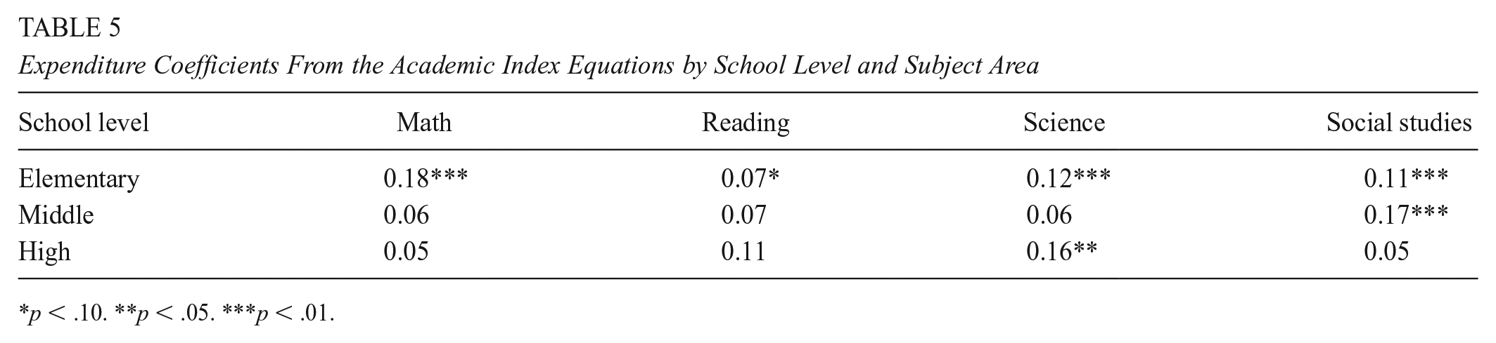
p < .10. **p < .05. ***p < .01.
We use the coefficients from the academic index models and the net expenditure effects presented in the previous section to estimate the performance impacts of the homestead exemption (Table 6). Specifically, we assume that the percentage changes in spending brought about by the exemption at the school level are equal to the percentage changes at the district level. This approach is justifiable provided that expenditure changes tend to be allocated to schools within a district in proportion to their initial budget shares. Since the net expenditure effects for the district with the 5th and 50th percentile exemption loss rates are near zero, the impacts on academic performance are also negligible. For the district with the 95th percentile exemption loss rate, the achievement impacts are larger but still quite small. The net increase in expenditure attributable to the homestead exemption leads to increases in the elementary math, social studies, and science, middle school social studies, and high school science in the neighborhood of one thousandth of a standard deviation. We see similar impacts for districts in which the median voter is likely to have been a claimant. These impacts are small relative to many interventions that have been studied by education researchers and economists. 6
Homestead Exemption Impacts on Elementary, Middle, and High School Academic Performance, Standard Deviations

Conclusion
Tax offsets such as Kentucky’s homestead exemption for the senior and disabled are appealing to policymakers since they potentially enhance the vertical equity of the combined state–local tax system while scoring political points with senior voters (a relatively engaged group) at no apparent cost to the state. However, because of the role that taxable property wealth plays in the generation of local revenues and in many state aid formulas, property tax relief programs such as Kentucky’s homestead exemption can have unintended consequences, particularly for rural districts since they tend to have above-average densities of disabled and senior residents.
In this study, we examine the impact of the homestead exemption in Kentucky on school district current expenditures, property tax rates, and academic achievement. We find that the exemption influences school district expenditure through price and income effects but that these impacts tend to be offsetting. In districts where the median voter is not a claimant, district-wide use of the exemption erodes the tax base, which increases the median voter’s share of the cost of locally financed education spending. This tax price increase puts downward pressure on the median voter’s demand for K–12 education spending. The tax base erosion due to the exemption increases state aid per-pupil due to Kentucky’s progressive aid formula. The additional aid places upward pressure on demand for education spending. When the median voter is not a claimant, the higher tax price increases the value of state aid to the median voter, which enhances the positive aid-driven income effect. The interplay between the price and income effects is different in districts where it is likely that the median voter is a claimant. Though the exemption greatly reduces the tax price of the median voter and increases the amount of state aid received by the district, the price reduction decreases the value of state aid to the median voter, which offsets the positive price effect. The net effect on expenditure depends on the relative magnitudes of the price and aid-driven income effects. In our analysis, we find that the exemption price elasticity is modest. Consequently, the price effect of the exemption on expenditure is negligible in the vast majority of areas where the fraction of property wealth that is exemptible is small and it is almost completely offset by the aid effect. In areas where the exemption claims a large fraction of property wealth, but the median voter is not likely to claim the exemption, the median voter’s tax price is significantly higher but due to the low price elasticity, the increase in state aid to the district, and the increased value of aid to the median voter due to the price increase, these districts experience modest net gains in expenditure. In districts where it is likely that the median voter is a claimant, the exemption greatly reduces the tax price of the median voter and increases the amount of state aid, but the price reduction reduces the benefit that the median voter derives from aid to a large enough degree that the net increase in expenditure is modest. None of the estimated expenditure increases are large enough to produce substantial improvements in student achievement. Nor do they produce property rate increases high enough to significantly cut into the tax relief received by senior and disabled homeowners.
Overall, the results suggest that Kentucky’s homestead exemption provides relatively generous tax relief to senior and disabled homeowners without significantly reducing the resources available to the vast majority of districts or affecting the resource and academic achievement gaps between rural and nonrural districts. This is primarily due to the offsetting effect of additional state aid and to the low-price elasticity associated with the exemption. The modest magnitude of the price elasticity could be the result of the low salience of the exemption among nonclaimants. Another possible contributing factor is the minimum local effort requirement that districts in Kentucky must meet to receive funding from SEEK, the state’s minimum foundation grant program. Another critical contextual factor uncovered in this study is the exclusive use of relative taxable property wealth to measure local fiscal capacity. The examination of the impacts of exemptions for the senior and disabled in states with less stringent local effort requirements and funding formulas in which relative taxable property wealth plays a less central role would sharpen our understanding of the impacts of this important tax relief mechanism on school district budgets.
Supplemental Material
sj-docx-1-ero-10.1177_2332858420988712 – Supplemental material for The Effects of Homestead Exemptions for Seniors and Disabled People on School Districts
Supplemental material, sj-docx-1-ero-10.1177_2332858420988712 for The Effects of Homestead Exemptions for Seniors and Disabled People on School Districts by Alex E. Combs and John M. Foster in AERA Open
Footnotes
Notes
Authors
ALEX E. COMBS is an assistant professor of public administration and policy at the University of Georgia School of International and Public Affairs. His research focuses on state financing of higher education and K–12 school finance equalization.
JOHN M. FOSTER is an associate professor in the Department of Public Administration and Policy Analysis at Southern Illinois University, Edwardsville. His research interests include public finance and budgeting, particularly at the state and local levels, quantitative research methods, education policy, program evaluation, policy analysis, and public sector economics.
References
Supplementary Material
Please find the following supplemental material available below.
For Open Access articles published under a Creative Commons License, all supplemental material carries the same license as the article it is associated with.
For non-Open Access articles published, all supplemental material carries a non-exclusive license, and permission requests for re-use of supplemental material or any part of supplemental material shall be sent directly to the copyright owner as specified in the copyright notice associated with the article.