
Abstract
Although numerous survey-based studies have found that students who identify as lesbian, gay, bisexual, or questioning (LGBQ) have elevated risk for many negative academic, disciplinary, psychological, and health outcomes, the validity of the types of data on which these results rest have come under increased scrutiny. Over the past several years, a variety of data-validity screening techniques have been used in attempts to scrub data sets of “mischievous responders,” youth who systematically provide extreme and untrue responses to outcome items and who tend to falsely report being LGBQ. We conducted a preregistered replication of Cimpian et al. with the 2017 Youth Risk Behavior Survey to (1) estimate new LGBQ-heterosexual disparities on 20 outcomes; (2) test a broader, mechanistic theory relating mischievousness effects with a feature of items (i.e., item response-option extremity); and (3) compare four techniques used to address mischievous responders. Our results are consistent with Cimpian et al.’s findings that potentially mischievous responders inflate LGBQ-heterosexual disparities, do so more among boys than girls, and affect outcomes differentially. For example, we find that removing students suspected of being mischievous responders can cut male LGBQ-heterosexual disparities in half overall and can completely or mostly eliminate disparities in outcomes including fighting at school, driving drunk, and using cocaine, heroin, and ecstasy. Methodologically, we find that some methods are better than others at addressing the issue of data integrity, with boosted regressions coupled with data removal leading to potentially very large decreases in the estimates of LGBQ-heterosexual disparities, but regression adjustment having almost no effect. While the empirical focus of this article is on LGBQ youth, the issues discussed are relevant to research on other minority groups and youth generally, and speak to survey development, methodology, and the robustness and transparency of research.
Keywords
While much survey-based research suggests that students who identify as lesbian, gay, bisexual, or questioning (LGBQ) are at elevated risk for a wide variety of negative outcomes—including suicide attempts, drug and alcohol use, sexual risk taking, being bullied, and facing disciplinary action (e.g., Centers for Disease Control and Prevention [CDC], 2016; Espelage, Aragon, Birkett, & Koenig, 2008; Mittleman, 2018; Robinson & Espelage, 2011; Russell, Sinclair, Poteat, & Koenig, 2012; Saewyc et al., 2004)—recent research has called into question the validity of the data on which many of these claims are based (e.g., Cimpian, 2017; Cimpian et al., 2018; Robinson-Cimpian, 2014; cf. Savin-Williams & Joyner, 2014a, 2014b; but cf. Fish & Russell, 2018; Katz-Wise, Calzo, Li, & Pollitt, 2015; Li, Katz-Wise, & Calzo, 2014). More specifically, the research challenging the validity of the data argues that some of the youth completing the surveys may have been “jokesters” or “mischievous responders” who provided dubious responses possibly because they found it funny to claim they were not heterosexual on a survey and also to make other bogus claims about their risk and misconduct (Cimpian et al., 2018; Robinson-Cimpian, 2014; cf. Savin-Williams & Joyner, 2014a, 2014b). For example, a student who identifies as heterosexual and does not use drugs may find it amusing to report on a survey that he identifies as gay and uses drugs often and heavily, thereby inflating estimates of gay-identified youth using drugs (see Fan et al., 2006, for similar argumentation and evidence with respect to adopted, foreign-born, and disabled statuses). Such claims of invalid survey data from youth leading to elevated risk profiles are not new (see, e.g., Cornell, Klein, Konold, & Huang, 2012; Cornell & Loper, 1998; Cross & Newman-Gonchar, 2004; Fan et al., 2006; Furlong, Sharkey, Bates, & Smith, 2004; Rosenblatt & Furlong, 1997); however, there is a new and increasing emphasis on how data invalidity can differentially affect estimates of minority-group risk, particularly when it is challenging or impossible to verify responses, such as in the case of LGBQ identification. Because of their systematic patterns of extreme reporting and their propensity to (falsely) report minority-group membership, the bias introduced into estimates by mischievous responders is distinctly different from other forms of misreporting bias such as haphazard responding and misunderstanding of terminology, and can exert extreme bias into estimates of minority-group well-being (Cimpian, 2017; Fan et al., 2006; cf. Groves, Fowler, Couper, Lepkowski, & Tourangeau, 2011).
It is imperative to understand and appropriately address mischievous responders for at least three reasons, all of which we discuss in this article: (1) Mischievous responders lead to incorrect estimates of the risk of minority groups (e.g., LGBQ youth, transgender youth, racial/ethnic minorities, students with disabilities) and impede our understanding of how to improve outcomes for these subgroups. (2) Survey designers need to know what types of items are particularly susceptible to mischievous responding. (3) Methodologists (and applied researchers) need to know the best ways to detect and reduce the effects of mischievous responding. Thus, the study of mischievous responders cuts across many aspects of education and social science research. This article will be of interest to researchers of LGBQ youth, the subject of our empirical investigation and of much of the current debates around mischievous responders. But it will also be of interest to survey designers and methodologists, as well as to researchers of other subgroups or of youth well-being in general.
In this article, we expand the field’s understanding of the effects of potentially mischievous responders in three ways: First, we perform a preregistered replication of Cimpian et al. (2018) with a recently released data set collected by the CDC, which informs how potentially mischievous responders affect estimates of LGBQ-heterosexual disparities on 20 commonly examined outcomes in a data set containing N = 108,093 student survey records in its final analytic form. We hypothesize that the removal of potentially mischievous responders will lead to significant reductions in disparities, on average, as soon as 1% of observations are removed, with larger reductions for males than females. Second, we replicate Cimpian et al.’s (2018) analysis exploring the relationship between item response-option extremity and the effects of mischievous responders, providing new large-scale evidence to a broader theory about the types of items and their response options that are most likely to be influenced by mischievous responders—this has implications well beyond LGBQ-heterosexual disparities, and can also help researchers think about how to address mischievous responding in the early stages of research. We hypothesize that disparities for items with relatively fewer respondents choosing the most extreme option (e.g., selecting “40+ days” for heroin use) will be more affected by screening out likely mischievous responders than items with more frequently selected extreme options (e.g., reporting feeling sad). This is because, having selected the extreme option for both types of items, mischievous responders will make up a disproportionately large share of extreme response selectors for items of the former type. Third, we provide a direct empirical comparison of the methods proposed—and implemented in the literature—to address potentially mischievous responders in a single data set, thereby eliminating one source of variability in comparing effects across different published papers (and their different data sets used), as well as providing insights to the field on when different methods reach similar conclusions about disparities. This component of the study is more exploratory, and we therefore make no predictions regarding methodological differences. Finally, we provide some guidance to researchers on how to combine preregistration practices and sensitivity analyses to improve the transparency of addressing data-validity threats from mischievous responders.
The Importance of Data Validity for LGBQ Research in Education
Research on LGBQ (and more broadly, LGBTQ) youth in education has been receiving increasing focus as of late, with a recent American Educational Research Association–published book (Wimberly, 2015b) and special issue of Educational Researcher (Cimpian & Herrington, 2017), as just two illustrations. Although both the book and special issue include a wide variety of research methodological perspectives, the general trend in education research on LGBQ youth has been a movement toward quantitative work (Brockenbrough, 2017). For instance, Wimberly (2015a, 2015b; Wimberly & Battle, 2015) calls for more quantitative research on LGBQ students. Thus, it is noteworthy that there have been several recent critiques from across methodological perspectives regarding how quantitative research chooses to categorize LGBQ youth in education research, yet it is valued by the education research community (Brockenbrough, 2017; Cimpian, 2017; Mayo, 2017). Indeed, if we are experiencing an increasing quantification of LGBQ research in education, we must ensure that the research is valid and not valued simply because it is quantitative. As seen in many research studies (for critiques, see Gelman & Loken, 2014; Simmons, Nelson, & Simonsohn, 2011), quantitative education researchers of LGBQ youth make many choices throughout the research process that can affect the findings. Because the presence of mischievous responders calls into question the validity of the data as well as any associated findings, we hope to draw attention to the choices regarding data validity and mischievous responders, as well as illustrate how these choices affect outcomes, while providing guidance on how to make the research choices more transparent.
It is also worth noting that, in an era of growing importance of administrative data sets for education research (Dynarski & Berends, 2015), LGBQ status is distinctly different from variables like race/ethnicity, sex, special education status, and English learner status because LGBQ status is not collected in administrative data sets. Thus, large-scale quantitative education research on LGBQ youth relies almost exclusively on the type of data gathered through anonymous self-administered questionnaires such as the one that is the focus of this article. 1
Screening, Its Different Purposes, and Assumptions Required
Before elaborating on the specific contributions of this article, it is important to note the broad assumptions required of any analysis with self-administered questionnaire data, and also to distinguish the general assumptions of the techniques we will discuss here from those of other data-validity methods in the literature. In doing so, we also hope to clarify why we are focusing on this specific set of data-validity sensitivity analyses.
Implicit in any data analysis with self-administered questionnaire data are assumptions about the validity of the data. Retaining all of the data, as many researchers do, assumes that the data are valid as they are. Removing questionable observations also makes assumptions, which vary by the method used and the nature of the analysis. Some data-removal techniques focus on assessing the variability in survey responses (e.g., Cross & Newman-Gonchar, 2004; Meade & Craig, 2012; Shukla & Konold, 2018). For example, one way Shukla and Konold (2018) identified suspect responses was by examining the variability within individuals in their responses to items that are part of a common construct scale—that is, we would expect a relatively small range of variability within an individual when responding to items that tap into the same construct—and then using latent profile analysis to identify and remove individuals who exhibited high levels of response inconsistency across seven different constructs. A method such as this identifies cases on their responses to outcome items of interest (e.g., academic press), whereas the typical screening responses we will focus on identify unusual cases based on responses to items that are not outcomes of interest (e.g., height). Other data-removal methods ask respondents to rate how truthful they were in their responses (e.g., Cornell et al., 2012; Jia, Konold, Cornell, & Huang, 2018; Shukla & Konold, 2018), thereby making the assumption that the respondents will truthfully state how untruthful they were earlier in the survey; however, it should be noted that reported truthfulness does correlate with more complex methods of detecting response-inconsistent data (Shukla & Konold, 2018).
These examples illustrate some dimensions on which the screeners we examine differ from some other approaches, but there are also important differences in their intent, which correspond to different required assumptions. For instance, the intent of many researchers interested in removing invalid data is to obtain a more accurate measure of an outcome globally, that is, across all groups in the data (e.g., Cornell et al., 2012; Furlong et al., 2017; Jia et al., 2018; Meade & Craig, 2012; Shukla & Konold, 2018). When researchers seek to obtain a global estimate (e.g., bullying experienced by all students), then the assumption when screening out observations is that the screener itself does not introduce bias into the global estimate—in other words, the assumption that screening has no global impact that would introduce bias into the estimate of the true overall value. By contrast, researchers interested in comparing groups (e.g., differences between LGBQ- and heterosexual-identified students in reported experiences of bullying) need only make the weaker assumption of no differential impact of screening on the groups being compared. This assumption requires that the screening technique does not introduce bias into the estimate for one group differently than for the group to which it is compared.
Thus, the assumptions required for data removal are weakened when making comparisons across groups, making data-removal in the case of comparisons less assumption-laden (though there are still assumptions, which we will discuss in detail later). The tradeoff, however, is that the assumptions required for valid data-removal in the case of one group comparison (e.g., LGBQ-heterosexual disparities) may not be plausibly satisfied for a different group comparison (e.g., disabled–non-disabled disparities) and may not be plausible more globally. For instance, Robinson-Cimpian (2014) assumed that actual LGBQ- and heterosexual-identified youth should not differ in terms of reporting blindness or deafness, and so he included those items in his screener when estimating LGBQ-heterosexual disparities; however, those same items of blindness and deafness are expected to differ between disabled and non-disabled students, and so those items were excluded from his screener when estimating disabled–non-disabled disparities because their inclusion would render implausible the assumption of non-differential impact.
Because the data-validity methodology literature is expanding and producing a large set of techniques (see, e.g., Fan et al., 2006; Jia et al., 2018; Shukla & Konold, 2018), it is necessary for us to hone the focus of this article on the most relevant techniques for the topic under study: LGBQ-heterosexual disparities. As such, we will focus our attention on this latter group of data-validity techniques, those which are primarily used to compare groups, and especially used to compare LGBQ and heterosexual youth (e.g., Cimpian et al., 2018; Fish & Russell, 2018; Mittleman, 2018; Robinson-Cimpian, 2014). We also focus on cases where data are anonymized, a common “best practice” when gathering sensitive data such as sexual identity (Badgett, 2009; Tourangeau & Yan, 2007), but one that prohibits verification through triangulation (Fan et al., 2006). These cases are perhaps the most methodologically challenging, require more assumptions, and arguably could benefit the most from replication and a comparison of existing methods.
The Present Article
As alluded to above, the current article has three components (separated as Studies). Study 1 is a direct replication of Cimpian et al. (2018) examining how potentially mischievous responders may affect estimates of LGBQ-heterosexual disparities. Study 2 further replicates Cimpian et al. (2018) by considering whether item-response extremity plays a role in those effects. Finally, in Study 3, we compare several common approaches for identifying and removing potentially mischievous responders. Here, we discuss each study in more detail.
First, replication is essential to ensuring that findings of a single study are not anomalous. Education researchers, and indeed the broader field of social scientists, are under increasing pressure to replicate and preregister studies to ensure the robustness of published findings (Fanelli & Ioannidis, 2013; Gehlbach & Robinson, 2018; Makel & Plucker, 2014; Open Science Collaboration, 2015). In this article, we conduct a direct replication of a recent study by Cimpian et al. (2018). The study by Cimpian et al. is an ideal one to replicate as part of a preregistered replication because Cimpian and colleagues used a data set that is part of a biannually collected series conducted by the CDC, and the 2017 iteration of the survey data was not yet released by the CDC when we submitted this manuscript as a registered report for consideration with our detailed analysis plan—thus, allowing for a preregistered hypothesis-testing study using a recurring national data set (Gehlbach & Robinson, 2018). However, Cimpian et al.’s (2018) study is important to directly replicate with new data for other reasons: First, the series the data come from are national and publicly available and have had a tremendous impact on the fields of education, psychology, and health (for some recent examples, see CDC, 2016, 2017; Clayton, Lowry, August, & Jones, 2016; Raifman, Moscoe, Austin, & McConnell, 2017; Vagi, Olsen, Basile, & Vivolo-Kantor, 2015; Zaza, Kann, & Barrios, 2016). Second, Cimpian et al.’s (2018) findings that LGBQ-heterosexual disparities may be substantially overestimated need to be replicated, given the impact the data series has on several fields and the questions raised about its validity, as well as what the findings could mean to methodological practices in survey-based comparisons, especially along sexuality dimensions. Thus, Study 1 of the present article is a direct preregistered replication of Cimpian et al. (2018) with the 2017 Youth Risk Behavior Survey (YRBS; for the preregistered form, go to https://aspredicted.org/sz9aa.pdf).
Second, Study 2 is also a direct preregistered replication of a component of Cimpian et al. (2018), testing the heterogeneity of effects on outcomes as related to extreme response selection. Cimpian and colleagues concluded that potentially mischievous responders affected LGBQ-heterosexual disparities on average, but there was substantial heterogeneity in how much the 20 outcomes were affected. Because mischievous responders are expected to provide low-frequency, extreme responses (Fan et al., 2006; Furlong, Fullchange, & Dowdy, 2017; Furlong, Sharkey, Bates, & Smith, 2004; Robinson-Cimpian, 2014), Cimpian and colleagues hypothesized that outcome items containing response options that were less frequently chosen (e.g., using heroin “40 or more times” in one’s life) would be the items most affected by the removal of potentially mischievous responders. Cimpian et al. (2018) found strong support for this hypothesis in the 2015 state and district sample, with large standardized Bs of 0.75 (ps < .001), among both males and females. Replicating this finding with the 2017 YRBS has implications for providing preregistered empirical support for this theory on how mischievous responders affect outcome estimates. In doing so, the work also provides survey developers and researchers with useful information regarding how they can mitigate the effects of mischievous responders in the early stages of survey research (i.e., survey development) instead of in the later stages (i.e., data analysis) through item construction. Therefore, Study 2 replicates the Cimpian et al. analysis of how item response option extremity relates to the effects of screening on individual outcome items.
Third, as discussed above, data-validity sensitivity techniques are gaining popularity in the study of LGBQ youth (e.g., Cimpian et al., 2018; Fish & Russell, 2018; Mittleman, 2018); yet, we would be remiss to conclude that all techniques make the same assumptions, that they all lead to the same conclusions, or even that the same techniques are applied similarly across different research studies. Thus, in addition to replicating the recent large-scale CDC-based study by Cimpian et al. (2018) with newly released data in Studies 1 and 2, this article compares the effects of the main data-validity sensitivity techniques used in the growing literature on LGBQ-heterosexual disparities in Study 3; and, it does so within a single data set, thereby eliminating one source of variability across different efforts to identify and address likely invalid data.
Method
Data
For all three studies, we use the publicly available YRBS data from the CDC: https://www.cdc.gov/healthyyouth/data/yrbs/data.htm. The students completed the paper-and-pencil questionnaires in school and answered questions related to their mental, emotional, sexual, and physical health. Following the approach of Cimpian et al. (2018), the final analytic sample is restricted to observations from the State and District YRBS data set with valid sampling weights and nonmissing values for sex and sexual identity. The CDC does not require surveying agencies to include the item on sexual identity; therefore, some entire states and districts are necessarily omitted from the analytic sample, just as in Cimpian et al. (2018).
Because we are primarily interested in replicating the methods and general findings of the earlier study, we use all states and districts that included the necessary sexual identity item in the 2017 survey, regardless of whether they were part of the 2015 sample in Cimpian et al. (2018). We do not expect estimates in this replication to be exact; instead, we are interested in the general trends of how estimates are affected by the removal of potentially mischievous responders. Nonetheless, there is substantial overlap in the jurisdictions that participated in the 2015 and 2017 YRBS. The majority of jurisdictions in the 2015 sample also appear in the 2017 analysis (i.e., 27 of 36 jurisdictions from 2015 are in the 2017 study), with four jurisdictions dropping out and nine being added (see Table 1). The final analytic sample was 108,093 students, of which 52,753 reported being males (6,219 of them reported LGBQ identifications) and the remaining 55,340 reported being females (12,228 of whom reported LGBQ identification; see Table 2).
Screener Items Administered by Each Jurisdiction

Note. Item 1: fruit; Item 2: salad; Item 3: potatoes; Item 4: carrots; Item 5: dentist; Item 6: asthma; Item 7: height. Items excluded from surveys administered in each jurisdiction are indicated with gray boxes, while included items are indicated with yellow boxes. Jurisdictions that did not participate in the survey year are indicated by black boxes. Boldfaced states and districts contained all 7 screener items in the 2017 data, and were used for all main analyses; analyses using all 2017 data (regardless of screener items included) are in Appendix B.
Demographic Characteristics of the Weighted Sample, by Reported Sex and Screener Threshold, Pooled Youth Risk Behavior Survey (YRBS) 2015, Pooled YRBS 2017, and the Subset of YRBS 2017 Who Were Administered All Seven Screener Items

In addition to providing details on the overlap in the publicly available jurisdictions meeting the study criteria from the 2015 and 2017 YRBS, Table 1 also shows which jurisdictions asked which of the seven items used in our screener. Jurisdictions asking all seven items in the 2017 YRBS appear in boldface. This is important for our comparison of methods in Study 3—while the boosted regression approach can more flexibly handle missing data, the presence of completely missing item-level data for entire jurisdictions unnecessarily complicates any comparison of methods. Thus, for Study 3, we restrict our analyses to only the subsample of jurisdictions asking all seven screener items (which we term the “full-screener” sample in our tables). For consistency across Studies 1, 2, and 3, the main text and focus of the article will be on the full-screener sample; however, for completeness, we also estimated all of Studies 1 and 2 for the full sample, and present those results in Appendix B. The results are generally similar.
The smaller full-screener sample (N = 51,524)—which is the main analytic sample for the remainder of this article—is demographically similar to the full sample (see Table 2). Furthermore, Table 3 illustrates that removal of observations due to screening itself (discussed below) does not alter the demographics of the sample in any substantial way, suggesting good generalizability regardless of sample restrictions and screening.
Demographic Characteristics of the Weighted Sample, by Reported Sex and Screener Threshold, Subset of Youth Risk Behavior Survey 2017 Who Were Administered all Seven Screener Items
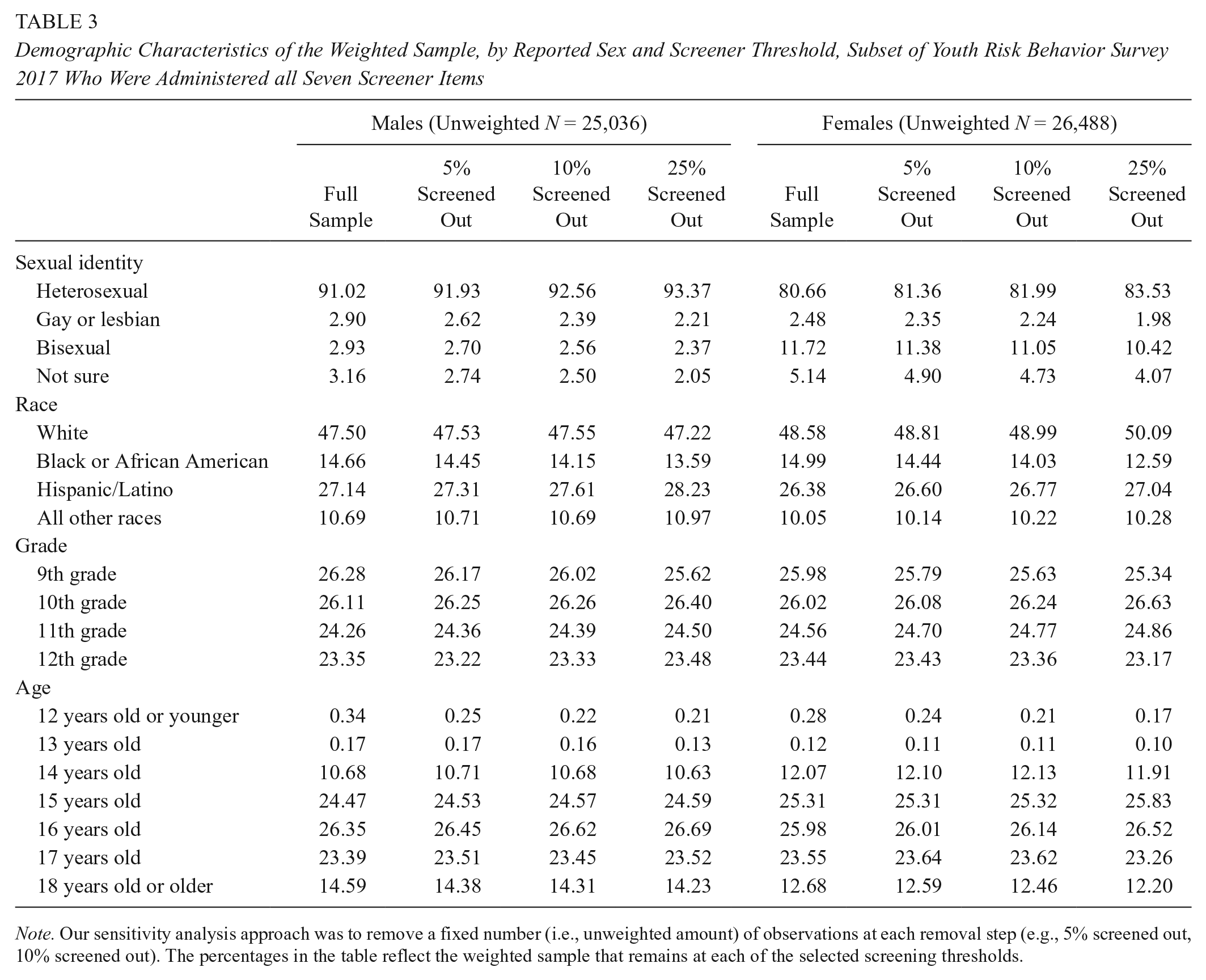
Note. Our sensitivity analysis approach was to remove a fixed number (i.e., unweighted amount) of observations at each removal step (e.g., 5% screened out, 10% screened out). The percentages in the table reflect the weighted sample that remains at each of the selected screening thresholds.
Outcomes
The YRBS includes a variety of items asking about high school students’ risk-taking behaviors and attitudes. Following Cimpian et al. (2018), for both Studies 1 and 2 (as well as for our comparison of methods in Study 3), we examine 20 items commonly studied in LGBQ research. Specifically, we include the following outcomes: rode in a car with a drunk driver, drove drunk, skipped school because felt unsafe, fought at school, was forced into sex, their partner forced sex on them, was bullied at school, felt sad/hopeless, considered suicide, planned suicide, attempted suicide, smoking, alcohol use, cocaine use, heroin use, ecstasy use, steroids use, number of sex partners, physical activity, and TV watching (see the Users Manual [CDC, 2018] for specific phrasing of items, also contained in Appendix C). All outcomes are coded continuously (e.g., reporting “20 to 39 times” is coded as 29.5).
Study 1: Direct Replication of Cimpian et al.’s (2018) Disparity Estimate Effects of Mischievous Responders
Identification of Potentially Mischievous Responders
Cimpian et al. (2018) extended the study of potentially mischievous responders to the largest sample to date, introduced the application of boosted regressions (a machine-learning technique) to identify unusual responding patterns, focused on LGBQ-heterosexual disparities, and found that potentially mischievous responders may account for an average of 46% of the LGBQ-heterosexual youth outcome disparity among males and 23% among females. We use their approach but applied to the 2017 version of the YRBS.
We identify potentially mischievous responders by exploiting relationships between reporting being LGBQ and ostensibly unrelated survey items. We expect no real relationship between sexuality and student characteristics such as height, asthma diagnosis, or dental history; likewise, the frequency with which individuals eat carrots, fruit, potatoes, or salad are not expected to be associated with sexuality in reality. However, some youth might find it funny to report extreme responses (Furlong et al., 2004; Furlong et al., 2017; Robinson-Cimpian, 2014), for example, reporting eating copious amounts of fruit, having never been to a dentist, being extremely tall, and being gay, even if all of these are untrue. Thus, the youth providing these mischievous responses create spurious relationships between the predictor (screener) items (e.g., salad consumption, asthma diagnosis) and sexuality, which can lead to unexpected and potentially misleading estimates of disparities. These screener items can then be used to identify youth providing the most unusual patterns of responses, and disparities in outcomes can be estimated without these potentially problematic responses included in the data.
As described in Cimpian et al. (2018), boosted regression (Friedman, 2001) is a machine-learning technique we can use to predict reporting LGBQ identification as a function of the specified screener survey items. We use the same seven screener items, location fixed effects to account for variation in survey item inclusion across jurisdictions, and YRBS survey weights (DuGoff, Schuler, & Stuart, 2014) as predictors. Following the boosted regression, each student is ranked by how likely they are to be a mischievous responder based on their response combination to the screener items. We use weighted linear probability models to obtain estimates of LGBQ-heterosexual disparities, with ordinal values recoded as continuous and include location fixed effects, using the full analytic data set. Then, we remove the top 1% of students (based on likely mischievousness) and reestimate the disparities. We repeat this process, sequentially removing the next 1% of data and reestimating the disparities, until 25% of the data have been removed. Additional details on the methods for Study 1 (and Studies 2 and 3) can be found in Appendix A.
Study 2: Direct Replication of Cimpian et al.’s (2018) Analysis of the Relationship Between Item Response-Option Extremity and Screening Effects
We directly replicate Cimpian et al.’s (2018) analysis exploring if the variation in screening effects across the 20 outcomes is related to how frequently respondents select the most extreme response options. Mischievous responders often choose extreme response options (Fan et al., 2006; Furlong et al., 2004; Furlong et al., 2017; Robinson-Cimpian, 2014), and items with fewer respondents overall selecting these options are then more susceptible to bias. We use a random effects model to predict the reduction in the estimate of LGBQ-heterosexual disparities between the model using all data and a given model with 1% to 25% of potential mischievous responders removed.
Study 3: Comparison of Post Hoc Mischievousness Reduction Techniques
While Study 1 detects mischievousness using one method—the most computationally complex and recently applied method—and Study 2 builds off of that detection method, Study 3 compares four methods for detecting mischievousness. Here, we briefly describe the various methods we will compare, then we discuss how we compare them; additional details are in Appendix A.
Method 1: Boosted Regression
This method is described above in Study 1.
General Notes for Methods 2 to 4
In all of the following approaches (i.e., anything other than the boosted regressions), the researchers must prespecify which response-options are considered tempting to mischievous responders. Note that this requires different assumptions than the boosted regression, which is important in two ways. First, while the boosted regression requires prespecifying items to consider (e.g., how often do you eat carrots?), the following methods require prespecifying item response-options to weight (e.g., eating carrots “4 or more times a day”). Second, the boosted regression will ignore the prespecified items if they are not helpful in differentiating between likely mischievous and nonmischievous respondents and it will give more weight to the items that are more helpful in differentiating; this is because there is no prespecification of how much to weight these items. By contrast, the following methods implicitly preweight the contributions of each pre-specified item response-option. That is, even if eating carrots “4 or more times a day” does not distinguish between reporting to be in the minority versus majority group, it will contribute to the ranking of likely mischievousness simply because the response option is a low-frequency choice and was preidentified by the researchers as an unusual response option. Thus, assumptions about which items and which specific item response-options are selected play a larger role in Methods 2 through 4.
Regarding our prespecification of tempting item response-options for this analysis, the Cimpian et al. (2018) analyses suggest a set of response-options to the screener items that are unusual and suggestive of likely mischievous responders. Based on that study, Table 4 presents the list of response-options we deem suggestive of mischievous responding in the 2017 YRBS. 2 (These item response-options in Table 4 are also used for Methods 3 and 4.)
Prespecified Screener Items and Extreme Response-Options in the Subset of Youth Risk Behavior Survey 2017 Who Were Administered All Seven Screener Items

Note. The wording (and bolding) in the first two columns is taken directly from the 2017 Youth Risk Behavior Survey.
Method 2: Unconditional Probability-Based Ranking
This method multiplies all of the unconditional probabilities of the prespecified screener item responses-options together and then ranks observations by their multiplied probabilities (Robinson-Cimpian, 2014). Individuals who selected most of the lowest probability researcher-specified mischievous response-options are sequentially removed from the data at 1% intervals and disparities are reestimated.
Method 3: Count Based
The count-based removal of suspected mischievous responders is similar to the probability-based approach, except each prespecified low-frequency response-option receives equal weight. More simply, this approach just tallies up the number of low-frequency responses provided to the items in Table 4. The more low-frequency response options a respondent provides, the more likely they are to be mischievous, and these individuals are removed sequentially in 1% intervals as in all the methods described above.
Method 4: Regression Adjustment
The regression adjustment approach uses the values of P from the probability-based approach (see Appendix A), but statistically conditions on a function of P rather than remove observations based on the ranking of P. That is, there is no data removal and no reweighting of observations in any way in this method, which separates it from all the methods described above; there is simply a regression-based covariate adjustment. We explore the consequences of different functional forms of P on how the estimates of the disparities: linear P, natural log of P (used in Fish & Russell, 2018), and the quartic of the natural log of P (used in Robinson-Cimpian, 2014).
Comparing the Methods
First, for each method (except the regression-based ones [Method 4]), we estimate the change in the average LGBQ-heterosexual disparities from the model using the full analytic data set to the model that screens out the top 1% of data. This average change is the precision-weighted average of the change in the 20 outcomes and adjusted for the covariance matrix in the changes (e.g., not treating changes in suicidal-ideation disparities as independent from changes in suicide-planning disparities). At each percentage of data removal, we test whether the removal of suspect data had a larger effect via one data-validity method relative to the others. We are able to see when in the sensitivity analysis (i.e., data removal process) the various methods yield the same results. To compare Method 4 (i.e., the regression-based adjustments), which each yield only one estimate (as opposed to the range of estimates produced by Methods 1–3), we show where the various regression-based adjustments fall in relation to the various other methods.
Hypotheses
Hypotheses for Study 1 (Preregistered Replication)
Based primarily on the recent work of Cimpian et al. (2018), we make several predictions. We predict the removal of potentially mischievous responders, as identified through the boosted regression, will lead to significant reductions in LGBQ-heterosexual disparities averaged over the 20 outcomes. We predict these reductions will be significant as soon as the top 1% of observations are removed. We predict the reductions will be larger among males than among females, who have been found to demonstrate less mischievousness in surveys (Cimpian et al., 2018; Fan et al., 2006). We do not make predictions about the individual outcomes, but only about the average of the 20 outcomes.
Hypotheses for Study 2 (Preregistered Replication)
Based on the findings of Cimpian et al. (2018), we expect to replicate their findings that item response-option extremity is predictive of the magnitude of the disparity reductions experienced when screening out potentially mischievous responder, for both males and females.
Hypotheses for Study 3 (Exploratory)
We make no a priori predictions for Study 3. Based on prior research relating boosted regressions to propensity score matching (McCaffrey, Ridgeway, & Morral, 2004) and on the efficiency of boosted regressions over previous supervised machine-learning methods (Hastie, Tibshirani, & Friedman, 2017), we do suspect the boosted regression to be most efficient in identifying potentially mischievous responders (in this case, if mischievous responders were biasing estimates upward and if the methods to detect them were not introducing bias themselves, efficiency would translate into smaller disparity estimates reached when removing fewer observations). However, we refrain from making strong predictions, and we view this study as exploratory.
Results
Study 1
As hypothesized, the results of Study 1 indicate that the removal of potentially mischievous responders leads to a significant reduction in average estimated disparities. This reduction is significant when just 1% of observations are removed, and the reduction is much larger for males than females. We focus here on results for the subset of jurisdictions that administered all seven screener items. Analyses of the full data set demonstrate similar trends and are available in Appendix B (Figures B17–B19).
When using all of the data, the average LGBQ-heterosexual youth health outcome disparity was 0.33 standard deviations (SDs) (95% confidence interval [CI] [0.25, 0.41]) among males (see Table 5). Here, we focus on the results of the boosted regression, but Table 5 shows results for all methods. When we removed the top 1% of observations identified by the boosted regression as providing the most unusual response patterns to the screener items, the estimated disparity reduced to 0.30 SDs (95% CI [0.22, 0.38]), and the change in the disparity was itself statistically significant (as indeed, all the changes are that are presented in Table 5). The estimate decreased to 0.25 SDs (95% CI [0.17, 0.33]) when removing the top 5%, decreased to 0.21 SDs (95% CI [0.13, 0.30]) when removing 10%, and decreased to 0.16 SDs (95% CI [0.08, 0.24]) when removing 25%. That is, the average of the male LGBQ-heterosexual disparities was cut in half when removing the top 25% of students ranked by likely mischievousness, yet neither did this data removal substantially alter any demographics of the data set (suggesting good generalizability; see Table 3) nor did it appreciably reduce precision of the estimated disparities.
Estimates and 95% Confidence Intervals for Average LGBQ-Heterosexual Youth Health Disparities Across 20 Outcomes, Subset of Youth Risk Behavior Survey 2017 Who Were Administered All Seven Screener Items
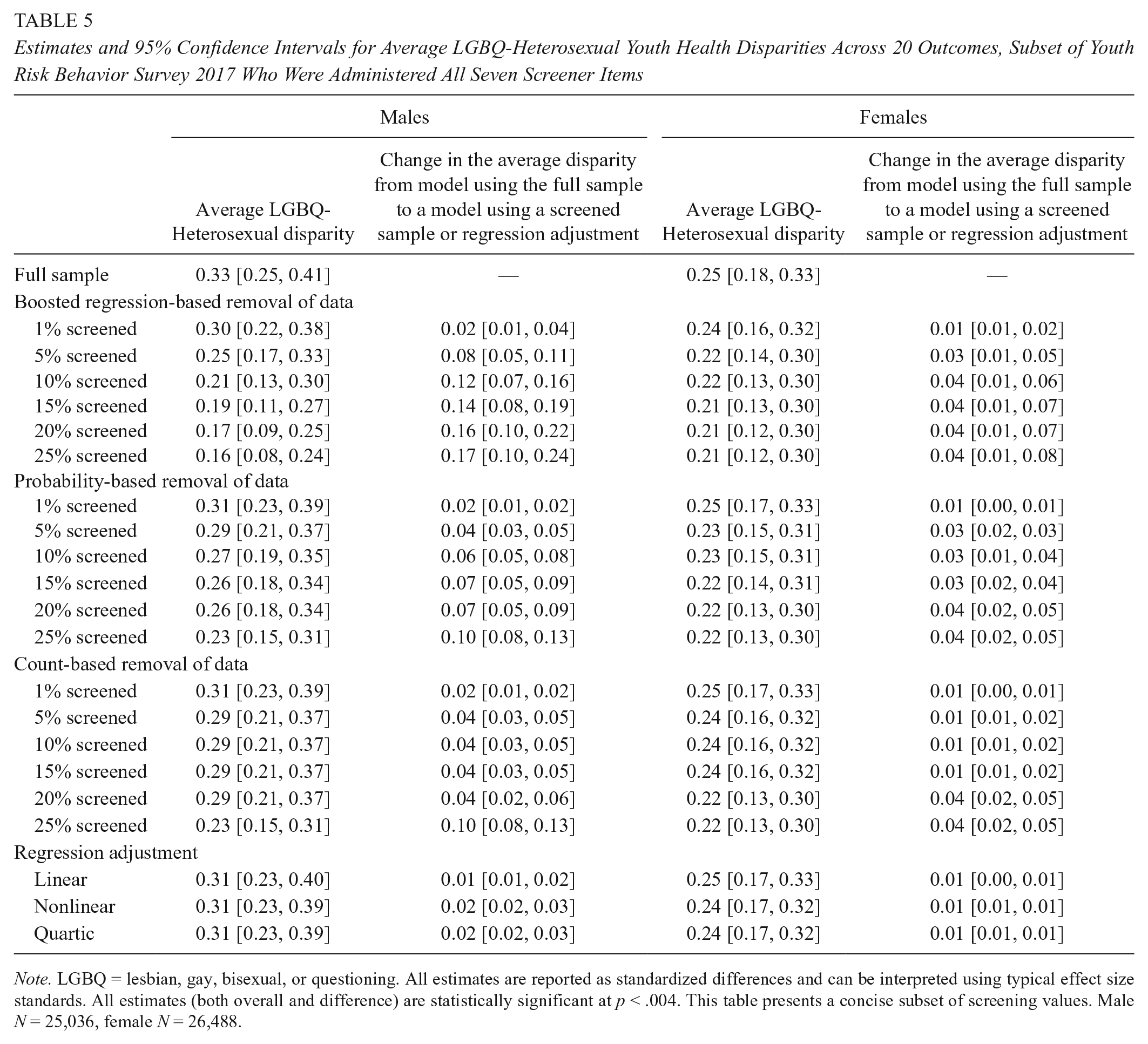
Note. LGBQ = lesbian, gay, bisexual, or questioning. All estimates are reported as standardized differences and can be interpreted using typical effect size standards. All estimates (both overall and difference) are statistically significant at p < .004. This table presents a concise subset of screening values. Male N = 25,036, female N = 26,488.
Among females, the average LGBQ-heterosexual estimated outcome disparity was 0.25 SDs (95% CI [0.18, 0.33]). Similar to the 2015 results presented in Cimpian et al. (2018), the changes in estimated disparities are much smaller among females than males. When removing the top 25% of observations, the estimated disparities decreased to 0.21 SDs (95% CI [0.12, 0.30]).
Both males and females demonstrated very similar patterns to the respondents of the 2015 YRBS. For both groups, estimates using the full sample were somewhat larger in 2015 than in 2017, with the average LGBQ-heterosexual disparity at 0.37 SDs (95% CI [0.29, 0.45]) for males and 0.31 SDs (95% CI [0.23, 0.38]) for females (Cimpian et al., 2018). Disparity estimates for males dropped much more substantially than for females in both survey administrations. In both 2015 and 2017, the difference for males between the full sample estimate and that based on 25% screened out was 0.17 (95% CI [0.11, 0.23] in 2015, and 95% CI [0.10, 0.24] in 2017). For females, differences were relatively smaller than males in both years, with the difference between the full estimate and that of the 25% screened out 0.07 (95% CI [0.03, 0.11]) in 2015 and 0.04 (95% CI [0.01, 0.08]) in 2017. While the estimated disparities are of course not identical, the patterns presented here using the 2017 YRBS are consistent with those Cimpian et al. (2018) identified in the 2015 YRBS.
Study 2
The results of Study 2 are also consistent with the findings of Cimpian et al. (2018). There is considerable variability in how screening affects estimated disparities across the 20 outcomes, and items with extreme response-options are predictive of the magnitude of disparity reductions.
As illustrated in Figures 1 and 2, while estimates of disparities for outcomes related to bullying and suicidal ideation were generally relatively stable for both boys and girls, disparities for drug- and alcohol-related outcomes were affected by the removal of potentially mischievous responders much more dramatically, particularly for boys. For example, among boys, the LGBQ-heterosexual boosted regression-based estimated disparity for heroin use showed an immediate steep decline, dropping from 0.55 SDs to 0.07 SDs on removal of the top 25% of responders. Disparities in alcohol and ecstasy use also dropped to 0.00 SDs among boys when removing the top 25% of responders. In contrast, the estimated disparity for reporting being bullied at school is virtually unchanged, moving only from 0.35 SDs to 0.34 SDs. Thus, it is unlikely that disparities in bullying and other relatively stable outcomes are driven by mischievous responders, whereas drug-related outcomes in particular are susceptible to their influence. While LGBQ-heterosexual disparity estimates among girls were generally more stable than the boys, similar patterns in drug- and alcohol-related outcomes are evident.

Average LGBQ-Heterosexual disparity among reported males in the full-screener subsample, by model, outcome, and percent of observations screened out.

Average LGBQ-Heterosexual disparity among reported females in the full-screener subsample, by model, outcome, and percentage of observations screened out.
In Figure 3, we explore the relationship between item response-option extremity and the average change in the estimated LGBQ-heterosexual disparity based on the boosted regression approach (see Table 6 for the extreme response options for each outcome). For both boys and girls, the smaller the proportion of respondents choosing the most extreme response option, the larger the change in the disparity (ps < .001). In both cases, drug-related outcomes notably have both very small numbers of students endorsing the most extreme response options and also demonstrate large changes in estimated disparities. In contrast, outcomes with relatively more commonly selected extreme response options also tend to have smaller changes in estimated disparities (e.g., bullied at school, physical activity). As with Study 1, our results for Study 2 demonstrate similar patterns to those found by Cimpian et al. (2018) with the 2015 YRBS.
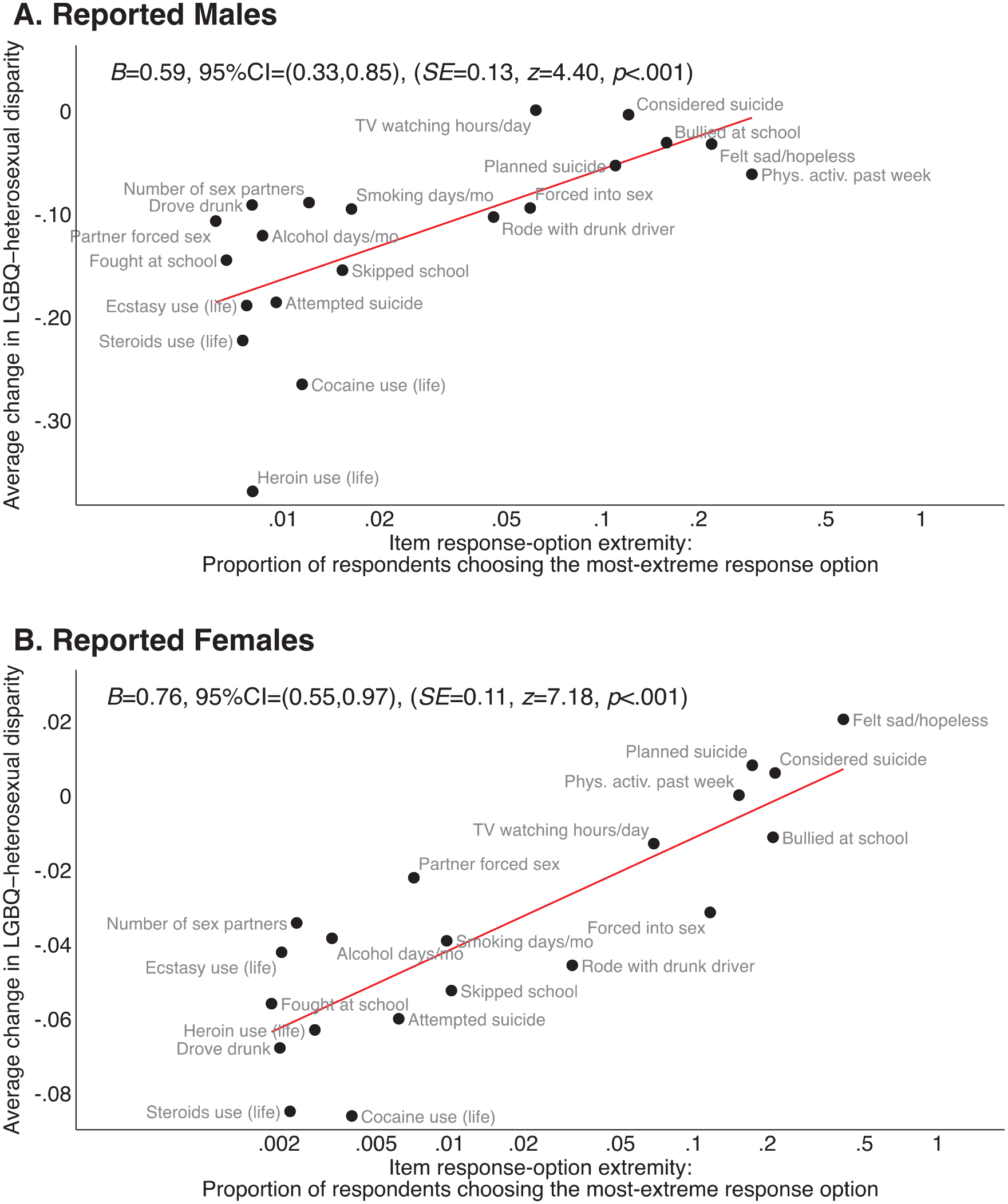
Relationship between how much an item-level disparity changed when screening mischievous responders and the item response-option extremity, in the full-screener subsample.
Outcome Items and Extreme Response-Options in the Subset of Youth Risk Behavior Survey 2017 Who Were Administered All Seven Screener Items

Study 3
In our exploratory analyses, we compared the average disparities estimated via the different methods for addressing potentially mischievous responders. The results differ somewhat by gender: Among males, there are clear differences among the methods; but among females, where likely mischievousness was tempered, so were the differences between the methods. In all cases, the boosted regression approach to identification followed by data removal led to statistically significantly smaller disparity estimates than did any of the regression-based adjustment methods (i.e., the methods that did not remove any data). Moreover, among males, the boosted regression approach followed by data removal led to smaller disparity estimates than did any of the other mischievous responder detection techniques followed by data removal. Figure 4 is a graphical illustration of the information presented in Table 5. In Figure 4, we see that the disparity line from the boosted regression is below every other data removal method, showing that it leads to the smallest average disparities at every estimation point.
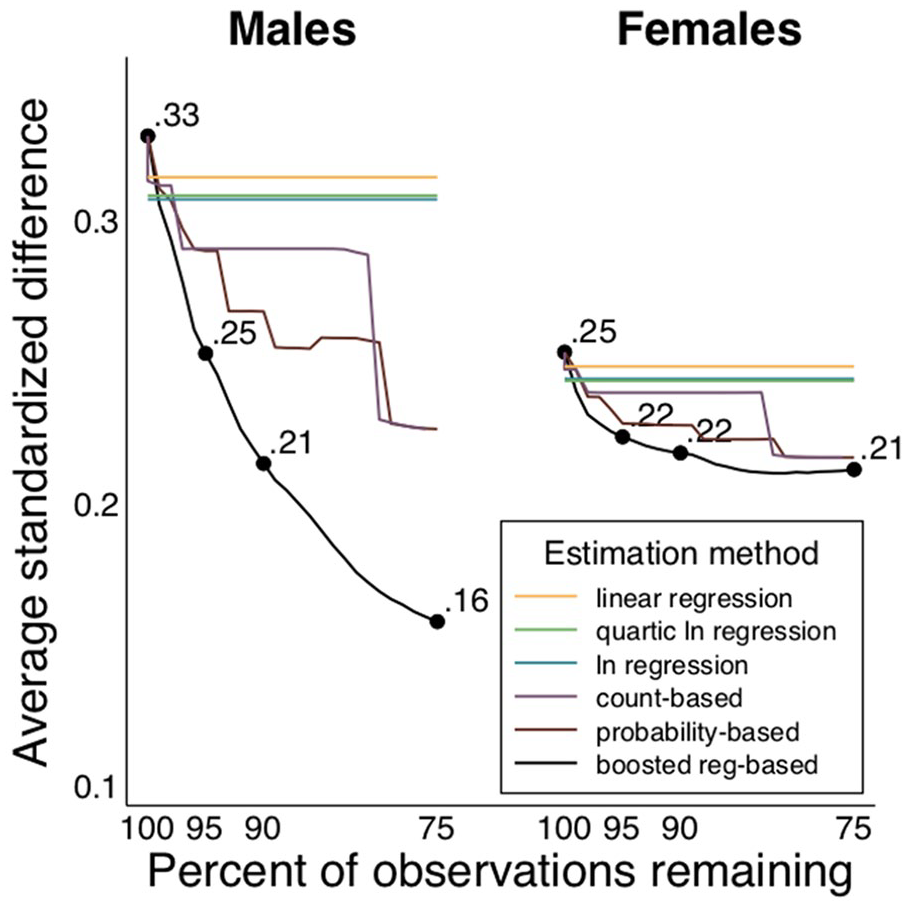
Average standardized LGBQ-Heterosexual disparities by gender, estimation method, and percentage of observations remaining, in the full-screener subsample.
Figure 5 directly compares the boosted regression estimates to each of the other estimates: Each line in Figure 5 represents a “difference in differences” of sorts, where the LGBQ-heterosexual difference from one method (e.g., probability-based approach, linear regression approach) is subtracted from the LGBQ-heterosexual difference from the boosted regression. The colored areas are 95% CIs for those difference-in-differences estimates, estimated via 1999 bootstrapped samples. Among males, the estimates from the boosted regression-based approach are statistically significantly different from those of all other approaches. For example, if 25% of the data were removed following the boosted regression identification method, the male LGBQ-heterosexual average disparity would be 0.16 SDs smaller than the estimate based on a regression-adjustment approach. Not only is that difference between methods statistically significant it also represents the practical difference of almost half of the unadjusted average LGBQ-heterosexual disparity; that is, the original male LGBQ-heterosexual average disparity using all data was 0.33 SDs, which reduced slightly to 0.31 SDs using the regression adjustment, but was cut in more than half to 0.16 SDs in the final boosted regression estimate.

Difference in average standardized LGBQ-Heterosexual disparities from the boosted regression approach, by gender, estimation method (compared with the boosted regression), and percentage of observations remaining, in the full-screener subsample.
Taken together, the results of Study 3 suggest that, if these methods are indeed identifying mischievous responders who are biasing disparity estimates, then (1) data removal eliminates more of the bias than do covariate adjustment approaches and (2) among the data removal approaches, the boosted regression approach to identifying likely mischievous responders leads to faster bias removal than do either the probability- or count-based approaches, reducing bias while being able to retain the greatest amount of observations. The differences between the approaches is more consequential when there is more potential for bias, such as in the case of males in the YRBS.
Discussion
This article replicates Cimpian et al. (2018) and finds consistent results regarding how potentially mischievous responders affect LGBQ-heterosexual disparities in Study 1. Furthermore, it adds a new empirical test for the theory of which items and response-options are most likely affected by mischievous responders in Study 2, helping survey developers plan in advance to mitigate the effects of mischievous responders, as well as helping applied researchers identify mechanisms linking these patterns together. For example, it may be at first confusing why suicidal ideation is not affected by mischievous responders but suicide attempts are, but this mechanism of item response-option extremity helps make sense of this pattern and an even broader set of patterns. That is, more students overall reported thinking about suicide than attempting it (especially repeated attempts); we replicate Cimpian et al.’s (2018) finding that likely mischievous responders will have undue influence on items where relatively fewer students choose the extreme response (e.g., suicide attempts) and that their influence is diluted when more students choose the extreme response (e.g., suicidal ideation). In addition to the preregistered replications, this article adds comparisons across the methods for identifying and either removing or adjusting for potentially mischievous responders in Study 3. The differences between the methods deserve additional focus, with growing concerns about ensuring data validity. We begin by discussing practical implications for nonresearchers, and then discuss the broader issue of research transparency.
Practical Implications for Interpreting Results
If researchers follow our suggestions, then practitioners, policy makers, and education decision makers would encounter articles and reports with a range of estimates for each outcome. This can be daunting and confusing, especially if the results from one model contradict those of another model. Importantly, if the results are inconsistent across the models, then the practitioners/policy makers/decision makers should use extreme care when interpreting the research studies and making real-world decisions (and researchers should clarify any data-validity concerns). We illustrate this point with a couple of examples from the current article. First, the disparity estimates were more stable across the models among females than among males, suggesting to decision makers that data validity may be less of an issue when reviewing survey data on females, and correspondingly, their data-based decisions regarding females are less sensitive to the specific model choices. The results using data on males, however, were more sensitive to modeling assumptions, thus decision makers will need to especially weight the plausibility of these assumptions when deciding how to proceed with policy and practice for males. Second, even among males, though, some disparity estimates were more stable than others. For instance, LGBQ males reported about one third of an SD higher likelihood of being bullied no matter the modeling assumptions; by contrast, the significance and/or magnitude of the estimated disparity depends on modeling assumptions for outcomes like fighting at school, skipping school, and a wide range of alcohol and drug uses. These patterns of (in)stability across the estimates may lead decision makers to conclude that the bullying disparity is not substantially influenced by potentially invalid data, and therefore, may require action on the part of educators to reduce this disparity. The data are less clear on the other outcomes, but we would not know that if we did not perform these sensitivity analyses. That is, these other outcomes may also require action, but the results of the survey data are inconclusive as to whether a disparity exists or its magnitude because the estimates change so much from model to model. Practically speaking, it is important to know if these estimated disparities are sensitive to modeling assumptions before resources are devoted to addressing and monitoring these outcomes by group.
Data Validity and Research Transparency
In the vein of the theoretical critiques in the recent special issue of Educational Researcher (see, e.g., Brockenbrough, 2017; Cimpian, 2017; Love, 2017; Mayo, 2017), this article also challenges—empirically—the assumptions implicit in much quantitative education research on LGBQ youth (see also, Robinson-Cimpian, 2014). Yet, this work pushes the empirical work a step further by providing direct comparisons of methods used for assessing data validity, and in doing so, illustrates that even seemingly similar work intended to reduce bias can lead to different conclusions based on the assumptions the researchers make throughout the analysis stage. This sort of methodological questioning extends well beyond the LGBQ (and LGBTQ+) research literature, to disparities related to other majority-minority comparisons, and even to the broader discussion of general data validity. In each study, researchers are making choices about overall and differential data validity.
We can think of these various researcher choices—perhaps charitably—as confronting and reducing messiness for a more distilled and coherent final result, or we can think more in the terminology related to registered reports and replication, such as “the garden of forking paths” (Gelman & Loken, 2014) or “researcher degrees of freedom” (Simmons et al., 2011), where researchers have many opportunities throughout the research process to tweak their findings to reach statistical significance (or in the case of LGBQ-heterosexual disparities in the presence of mischievous responding, opportunities to avoid losing statistical significance). Indeed, the movement toward preregistered studies is driven by a goal to prespecify the details of the methods, to reduce the forking paths and degrees of freedom—all with the objective of transparency in research (Gehlbach & Robinson, 2018). In the case of potentially mischievous responders, there are a tremendous number of researcher degrees of freedom, from deciding whether to do anything at all about the issue of data validity, to which method(s) to use for detection, to which items (and response options) to include in the screener, and possibly, to which observations should be removed.
At this point in the field’s understanding of the effects of mischievous responders, we would recommend a combination of preregistration and presenting a range of results under different assumptions. For example, if researchers have decided they want to address the issue of potentially mischievous responders using boosted regressions, then they can preregister the specifics of the boosted regression parameters (e.g., tuning, bagging, cross-validation stopping rules) and the items included in the boosted regression (e.g., height, carrot eating). We would caution, however, against prespecifying when to stop removing observations based on a rigid percentage of data (e.g., only 1% of data) or overly strict screening criteria (e.g., only removing cases if they provided all extreme responses to 10 screener items). Instead, we follow the recommendation of Cimpian et al. (2018) and recommend that researchers present a range of estimates based on different thresholds for screening out observations (e.g., estimates arrived at retaining all data, retaining 99%, 95%, 90%, and so on). Once mischievous responders are removed from the data, the estimated LGBQ-heterosexual disparities should converge to a relatively stable estimate (Cimpian et al., 2018; Robinson-Cimpian, 2014), but determining in advance when that stability will be achieved is futile. If the estimates do not converge, this is also useful information for consumers of researchers, so that they can assess the robustness of the findings on which they are basing education, health, and policy decisions. Thus, we would urge researchers to be more transparent in their dealings with issues of data validity, and this transparency may take the form of a combination of (1) preregistration to reduce researcher degrees of freedom in advance and (2) presenting a range of estimates that result from the remaining researcher degrees of freedom that could not be reasonably eliminated in advance.
Footnotes
Appendix A
Appendix B
Appendix C
2017 State and Local
Youth Risk Behavior Survey
This survey is about health behavior. It has been developed so you can tell us what you do that may affect your health. The information you give will be used to improve health education for young people like yourself.
DO NOT write your name on this survey. The answers you give will be kept private. No one will know what you write. Answer the questions based on what you really do.
Completing the survey is voluntary. Whether or not you answer the questions will not affect your grade in this class. If you are not comfortable answering a question, just leave it blank.
The questions that ask about your background will be used only to describe the types of students completing this survey. The information will not be used to find out your name. No names will ever be reported.
Make sure to read every question. Fill in the ovals completely. When you are finished, follow the instructions of the person giving you the survey.
Data Availability
To facilitate the use of screening analyses with the 2017 YRBS data, as well as to further increase the transparency of our own research, we make our main screening weights and code freely available for download from the Open ICPSR website (![]() ). Thus, researchers can readily assess the robustness of their own findings with the 2017 YRBS data, as well create their own screener with the 2017 YRBS or use our code as a template for a different data set.
). Thus, researchers can readily assess the robustness of their own findings with the 2017 YRBS data, as well create their own screener with the 2017 YRBS or use our code as a template for a different data set.
1.
There are exceptions, of course, such as Mittleman’s (2018) recent use of the Fragile Families data set to examine differential disciplinary practices by sexual identity. The structure of that data set is more similar to the Add Health data set—which has contributed substantially to the LGBQ student literature, though its validity has recently come into question (Savin-Williams & Joyner, 2014a, 2014b; but cf. Fish & Russell, 2018; Katz-Wise et al., 2015; Li et al., 2014)—with nonanonymized longitudinal data, different modes of survey administration, and questions of relatives and educators. It is worth noting, though, that despite the different nature of Mittleman’s data, he too uses a screener, suggesting the growing importance of validity screening with LGBQ status data across data sets.
2.
Note that these extreme response options are based on the pattern of results from ![]() , which used a boosted regression to identify likely mischievous responders. Thus, all of the other methods (i.e., Methods 2, 3, and 4) benefit from this knowledge, and consequently, perform better than they would if they did not have this knowledge from the boosted regression results in the study we are replicating. That is, if anything, the comparison of our methods is likely biased toward zero.
, which used a boosted regression to identify likely mischievous responders. Thus, all of the other methods (i.e., Methods 2, 3, and 4) benefit from this knowledge, and consequently, perform better than they would if they did not have this knowledge from the boosted regression results in the study we are replicating. That is, if anything, the comparison of our methods is likely biased toward zero.
Authors
JOSEPH R. CIMPIAN, PhD, is an associate professor of economics and education policy at the New York University Steinhardt School of Culture, Education, and Human Development, Kimball Hall, 2nd floor, New York, NY 10003;
JENNIFER D. TIMMER, PhD, is an Institute of Education Sciences postdoctoral research fellow in the Department of Leadership, Policy, and Organizations at Vanderbilt University, Peabody College, PMB 414, 230 Appleton Place, Nashville, TN 37203;