Sage Journals: Discover world-class research

Abstract

As state governments seek to improve the performance of institutions of K–12 and higher education, they often adopt educational policies that have similar names but different characteristics across states and with variations over time within states. Yet quantitative analyses generally examine the absence or presence of an educational policy instead of diving into details such as the dosage or percentage of funding tied to a policy or the specific groups being targeted by the implementation of the policy. The aim of this article is to provide guidance for education policy researchers in constructing and analyzing detailed data that can inform the design of state-level policies, using state performance-based funding policies in public higher education as an example. We also show how to conduct difference-in-differences analyses with continuous treatment variables in order to take advantage of more-nuanced data and better understand the context in which policies are effective (or ineffective).

Keywords

state policies data collection difference-in-differences analyses

The role of state governments in shaping educational policies is arguably stronger today than at any point in the past two decades. The passage of the Every Student Succeeds Act in 2015 to replace No Child Left Behind curtailed the power of the U.S. Department of Education over states’ K–12 educational practices after years of critiques from both sides of the political aisle (Dillon, 2011; Klein, 2016; Krane, 2007). In higher education, the Trump administration is moving to reverse a number of federal accountability provisions in higher education while many states are taking a more active role in attempting to improve colleges’ performance (Kelchen, 2018a).

A large body of research has shown that innovations in K–12 and higher education adopted in one state often spread to other states through the policy diffusion process (e.g., Hearn, McLendon, & Linthicum, 2017; Lacy & Tandberg, 2014; McDermott, 2003; Mintrom, 1997; Mokher & McLendon, 2009), but distinctions in local needs and political preferences often lead states to function as policy laboratories, approaching similar policy issues in a range of different ways (Elazar, 1972; Karch, 2007). As a result, qualitative and quantitative research in education has shown a great deal of heterogeneity in how states adopt and interpret educational policies (Dougherty, Natow, Pheatt, & Reddy, 2016; Wong, Wing, Martin, & Krishnamachari, 2018).

Yet many quantitative analyses in both K–12 and higher education classify complex state policies into a small number of basic classifications. Numerous empirical studies examining policies that vary considerably across states, such as charter school policies and higher education funding strategies, treat such policies as being binary in nature (e.g., Finger, 2018; Wong & Shen, 2002). Researchers often make these decisions for the purpose of methodological convenience: Quasi-experimental methods frequently used to generate causal estimates of policy impacts are easier to estimate using a binary treatment variable, and existing data sets often do not contain the detailed information required to construct a continuous treatment measure. Yet policy makers need to know how the details of state education policies affect student outcomes, as examining the simple absence or presence of a policy can obscure important details about which conditions make a particular policy effective (or ineffective).

Some studies provide a slightly more nuanced look at the data by placing states into a small number of groups based on similar policy characteristics (e.g., Kelchen, 2018b; Sjoquist & Winters, 2015). Collapsing heterogeneous policies into broad categories, however, leaves policy makers with little nuanced information about how to design state-level policies to meet their intended outcomes (and to mitigate potential unintended consequences). To fully understand the implications of different types of educational policies across states, researchers typically need to compile their own data sets capturing how policies have changed in each state over time. As Table 1 shows, a number of recent studies have begun to use this method to answer a range of questions. However, only some of these studies publish summary data at the state level, and few get into issues of variations in treatments within or across states. This slowly growing literature base represents a promising direction for informing policy, but researchers lack clear guidance on how to construct and analyze detailed state-level education policy data.

Table 1

Examples of National Studies on State-Level Educational Policies

Study	Years studied	Method	Outcomes	Policy data available in article or online appendix?
Performance funding
Gándara and Rutherford (2018)	1993–2014	Difference-in-difference	Underserved student enrollment	Yes
Kelchen and Stedrak (2016)	2003–2012	Multivariate regression	Institutional finances	No
Li (2018)	2003–2014	Difference-in-difference	STEM bachelor’s degrees	Yes
Merit aid
Doyle (2010)	1984–2005	Multivariate regression	State merit aid per FTE	No
Fitzpatrick and Jones (2016)	1990–2010	Multivariate regression	In-state and out-of-state attendance and residential migration	Yes
Kramer, Ortagus, and Lacy (2018)	1988–2009	Difference-in-difference	Tuition and fee levels	Yes
School accountability
Hanushek and Raymond (2005)	1992–2002	Multivariate regression	Math and reading scores	No
Springer (2008)	2002–2005	Multivariate regression	Math score gains	No
Wong et al. (2018)	2003–2011	Multivariate regression	Stringency of accountability policies	No
School finance reform
Card and Payne (2002)	1977–1992	Multivariate regression	Educational spending, SAT scores	Yes
Jackson, Johnson, and Persico (2016)	1955–1985 birth cohorts	Multivariate regression, instrumental variables	Educational and socioeconomic attainment	Yes

Note. STEM = science, technology, engineering, and mathematics; FTE = full-time equivalent.

In this article, we outline how to collect and analyze detailed data on state education policies in order to account for heterogeneity in how states adopt and implement policies, using state performance-based funding (PBF) policies in higher education as a case study of a complex educational policy that differs substantially across adopting states. We begin by offering a brief summary of PBF policies that tie state funding to student outcome metrics and considering how existing research has examined the effects of these policies. We then provide a step-by-step guide on how to construct detailed policy data sets that allow for more nuanced analyses of complex education policies, including a discussion of how to collect data using state education commission websites, budget documents, media coverage, and discussions with stakeholders in a way that can be replicated and expanded on by future researchers. We also provide examples of the data dictionary and data collection protocol as a practical guide for this work. Finally, we describe how researchers can leverage detailed data to extend common quasi-experimental methods, particularly difference-in-differences (DD) designs that are frequently employed to examine the impacts of state-level education policies, to provide more nuanced analyses and policy recommendations.

Case Study: Performance-Based Funding in Higher Education

The case study used throughout this article, PBF, is an increasingly popular higher education policy that ties a portion of state funding for public institutions to various student outcome metrics, with the goal of incentivizing colleges to operate more efficiently and improve student outcomes (Dougherty & Natow, 2015). As of 2017, 35 states connect at least a portion of their higher education appropriations to PBF (Hillman, Fryar, & Crespín-Trujillo, 2018), with additional states, such as California, either considering or transitioning to a PBF policy (Fain, 2018).

The structure and dosage of PBF policies vary considerably across participating states. For example, Michigan ties only 1% to 2% of higher education appropriations to performance-based outcomes, while Tennessee allocates 85% of higher education appropriations to performance (Snyder & Boelscher, 2018). Other states, including North Carolina, Michigan, and Ohio, tie different shares of funding to outcomes or use different funding formulas for 2- and 4-year colleges. A growing number of PBF-participating states have also introduced bonuses or premiums for graduating low-income, racial minority, or other at-risk students in order to achieve greater equity (Gándara & Rutherford, 2018; Kelchen, 2018a), but the amount of PBF allocated for equity considerations and the specific equity metrics being incentivized (e.g., low-income, minority, adult, at-risk students) also differ substantially across participating states (Jones et al., 2017).

Despite the growing presence of PBF policies, the majority of peer-reviewed academic research on the effectiveness of PBF policies has shown that adoption leads to null or negative effects on student outcomes (e.g., Hillman et al., 2018; Hillman, Tandberg, & Fryar, 2015; Umbricht, Fernandez, & Ortagus, 2017). However, most multistate analyses rely solely on binary indicators of PBF and are unable to account for distinctions between PBF policies (or changes to PBF policies once in place). The growing popularity of PBF combined with the lack of detailed policy data over time suggests the need for detailed descriptive and quasi-experimental analyses that move beyond binary indicators of complex educational policies. In the following section, we describe how to construct a detailed data set of state educational policies to be able to support such analyses.

Constructing a State Policy Data Set

One of the reasons why few researchers have constructed detailed data sets of state educational policies (and conducted analyses using detailed data sets) is the time-consuming nature of creating such a data set. Yet this sort of work is needed in order to accurately examine the effectiveness of different components of state educational policies and ultimately influence public policy discussions with nuanced, evidence-based recommendations for how to design effective educational policies.

In this section, we offer a step-by-step guide to constructing a detailed longitudinal state policy data set. The goal of this guide is to help advance the field of education research by offering exposure to the nuances and processes associated with collecting and using administrative data across policy-adopting states. Even though we present this guide as a linear process, researchers should expect to go back and make changes to their variables list and data collection process after they begin to collect data. However, our hope is that this guide helps researchers reduce the amount of time needed to produce a useful data set.

The first step is to determine the intended time period of the data set. In some cases, the time period to be examined will be clearly defined based on the first state to adopt a certain educational policy. In other cases, researchers may consider a natural break point related to when states changed their level of commitment to a policy, particularly for programs that have existed in some states for decades. Another option that is not ideal, but often necessary for researchers working with a limited budget, is to choose the years included in the data set based on issues of statistical power or the researcher’s available resources. Bringing older years of data into a data set may allow for more policy adoptions or changes in policy, but each older year of state policy data may come at a high cost to researchers due to the difficulty in gathering older records. In addition, researchers may consider focusing on relatively recent policy adoptions if the goal of the corresponding research is to influence ongoing policy discussions, as legislators and state educational agencies may not be as interested in an analysis that includes data on long-abandoned or since-revised aspects of educational policies.

In our PBF example outlined above, we chose to begin in 1997 because it allowed for a two-decade panel data set that balanced available resources with the ability to capture nearly all policy adoptions. While eight states adopted PBF between 1993 and 1996, all but one of these states abandoned PBF by 2002 (Dougherty & Natow, 2015). Finding details of these short-lived programs is exceedingly difficult, as little information on these programs are available on the Internet and many state education agencies lack the institutional memory to help fill in missing data. For the purposes of quasi-experimental analyses, we recommend that researchers collect available data on the absence or presence of a policy for several years prior to the beginning of the main policy data set and also collect information on available state-level and institution-level characteristics from sources such as the Common Core of Data or the Integrated Postsecondary Education Data System. This allows for comparisons of pretreatment trends and allows for the first years of detailed policy data to be used in analyses.

This decision should be immediately followed by creating a draft list of the variables of interest, or a data dictionary, that includes a clear description of each variable. Because the list of variables to collect should be based on theory and prior research, it may be necessary to collect data on policies to include not only the main variable(s) of interest but also covariates that could serve as confounding factors. For example, researchers interested in examining state charter school enrollment caps may wish to collect additional information on the landscape of school finance equity lawsuits, as that could potentially influence whether charter schools choose to operate within a state. The same data collection protocol identified above would still hold in such a situation, but the number of variables collected (and the time needed to collect those variables) would increase due to the need to account for additional contextual complexities that could otherwise threaten the internal validity of later analyses.

The focus in state educational policy data collection efforts should be to go beyond a simple binary indicator of a policy’s presence in a given year and attempt to measure the intensity or dosage of a policy. This dosage measure captures variations in policy adoption across states as well as within states over time, such as differences in levels of state funding tied to student outcomes or the types of metrics being considered. The typical variable of interest in the PBF literature has been the absence or presence of PBF at a given college or in a given state at a particular point in time, but a small body of recent literature has expanded the focus to examine the presence of bonus provisions for STEM (science, technology, engineering, and mathematics) or historically underrepresented student success (Gándara & Rutherford, 2018; Kelchen, 2018a; Li, 2018). A consulting firm, HCM Strategists, released a four-category typology of PBF formulas in fiscal years 2015, 2016, 2018, and 2019 that represented a slightly more nuanced classification of states’ PBF policies (e.g., Snyder & Boelscher, 2018; Snyder & Fox, 2016), categorizing participating states based on the percentage of funds at stake in a given sector and a few other details related to each state’s PBF formula. While such categorizations move the research community closer to understanding how key components of a particular policy affect outcomes, they may offer little specific guidance to policy makers seeking to better understand which aspects of an educational policy are effective in achieving the goals of the policy or legislative body.

Table 2 contains an example data dictionary, which shows researchers how to begin data collection efforts with the goal of measuring variations in dosage of PBF policies by including as much detail as practically possible. We first included both the dollar amount and percentage of state appropriations tied to institutional performance each year, as different analysts may find one of the two numbers more suitable for their analyses. We then collected details on the individual success metrics included in PBF systems, such as credit completions, retention, and the number of credentials awarded. To capture the presence of bonus provisions, such as bonuses for graduating underrepresented or STEM students, we also collected data on the amount and percentage of state appropriations tied to performance metrics associated with individual student subpopulations of interest.

Table 2

Data Dictionary for Performance-Based Funding (PBF) Policies With an Example State (Tennessee in Fiscal Year 2008)

Variable Name	Definition	Tennessee FY 2008
stateid	unique identifier for state	TN
state	state abbreviation	42
year	fiscal year being collected (e.g., 2016 is 2015–2016 academic year)	2008
pbf_authorized_any	0 if state does not have a PBF policy on the books in a given academic year; 1 if state does	1
pbf_funded_any	0 if state does not have a funded PBF system in a given academic year; 1 if state does	1
pbf_all_colleges	1 if state has PBF for all public colleges; 0 if no PBF or PBF for only 2-year colleges or for only 4-year colleges	1
pbf_4yr	1 if state has PBF for 4-year colleges; 0 if no PBF or PBF for only 2-year colleges	1
pbf_2yr	1 if state has PBF for 2-year colleges; 0 if no PBF or PBF for only 4-year colleges	1
pbf_other	1 if state has PBF for a specific set of colleges (e.g., PASSHE system in Pennsylvania); 0 if no PBF or PBF for only 4-year or only 2-year colleges	0
pbf_ipeds_pbf_colleges	IPEDS UnitID(s) for colleges subject to PBF policy in a given year	List UnitIDs here (not provided to save space)
approp_all_colleges	total state funding for public higher education	$1,361,977,000
approp_4yr	total state funding for 4-year colleges	$950,609,000
approp_2yr	total state funding for 2-year colleges	$229,123,000
pbf_pct_authorized_all_colleges	% of state funding authorized to be allocated based on performance for all colleges (may be different than actual allocation)	5.45
pbf_pct_authorized_4yr	% of state funding authorized to be allocated based on performance for 4-year colleges	5.45
pbf_pct_authorized_2yr	% of state funding authorized to be allocated based on performance for 2-year colleges	5.45
pbf_pct_all_colleges	% of state funding allocated based on performance for all colleges	4.134425
pbf_pct_4yr	% of state funding allocated based on performance for 4-year colleges	4.426520
pbf_pct_2yr	% of state funding allocated based on performance for 2-year colleges	6.211086
pbf_amt_authorized_all_colleges	amount of state funding authorized to be allocated based on performance for all colleges (may be different than actual allocation)	$74,227,747
pbf_amt_authorized_4yr	amount of state funding authorized to be allocated based on performance for 4-year colleges	$51,808,191
pbf_amt_authorized_2yr	amount of state funding authorized to be allocated based on performance for 2-year colleges	$12,487,204
pbf_amt_all_colleges	amount of state funding allocated based on performance for all colleges	$56,309,923
pbf_amt_4yr	amount of state funding allocated based on performance for 4-year colleges	$42,078,897
pbf_amt_2yr	amount of state funding allocated based on performance for 2-year colleges	$14,231,026
pbf_source	provide link to site(s) with information	Provide links
pbf_metricofsuccess	metrics for success an institution must meet in order to receive PBF	Student learning and outcomes, student satisfaction, student persistence, assessment outcomes
pbf_metricsvary	provide details regarding states that allow colleges to choose one or more metrics	N/A
pbf_targetedbonus	1 if has incentives for PBF premiums; 0 if no incentives for PBF premiums	0
pbf_percentofbonus	incentive based funds as a % of total funds	0
pbf_amountofbonus	amount of incentive-based funds	0
pbf_bonus_adults	1 if state has PBF bonus for adult enrollees; 0 otherwise	0
pbf_bonus_adults_notes	provide notes on how the state defines adults (and for which colleges/sectors)	N/A
pbf_bonus_lowincome	1 if state has PBF bonus for low-income enrollees; 0 otherwise	0
pbf_bonus_lowincome_notes	provide notes on how the state defines low income (and for which colleges/sectors)	N/A
pbf_bonus_minority	1 if state has PBF bonus for underrepresented minority enrollees; 0 otherwise	0
pbf_bonus_minority_notes	provide notes on how the state defines minority (and for which colleges/sectors)	N/A
pbf_bonus_acad_underprep	1 if state has PBF bonus for academically underprepared enrollees; 0 otherwise	0
pbf_bonus_acad_underprep_notes	provide notes on how the state defines academically underprepared (and for which colleges/sectors)	N/A
pbf_bonus_stem	1 if state has PBF bonus for STEM students; 0 otherwise	0
pbf_bonus_stem_notes	provide notes on how the state defines STEM (and for which colleges/sectors)	N/A
pbf_bonus_other	provide information about any other bonus groups	N/A
pbf_targetedbonus_notes	document details of PBF-targeted bonus (including dollar values/percentages tied to specific bonus metrics)	N/A
pbf_targetedbonus_source	provide link to site(s) with information	N/A

Note. PASSHE = Pennsylvania State System of Higher Education; N/A = not available; IPEDS = Integrated Postsecondary Education Data System; STEM = science, technology, engineering, and mathematics.

In Table 3, we include a sample of the data we collected for Tennessee in Fiscal Year 2008 as an example of what a data entry looks like for a state with a complicated PBF system. Even though Tennessee’s PBF policy was in place throughout the duration of the time period for which we collected data, the state made several substantive changes over time in both the amount and percentage of state funding tied to institutional performance metrics and therefore offers a useful example of variations over time in the characteristics and dosage of a PBF policy.

Table 3

Performance-Based Funding (PBF) State-Level Policy Data Set Construction Protocol

• Step 1: Set Google search timing ○ Change “Anytime” in the search options (just underneath and to the left under search bar when results are shown) to “custom range.” Use a custom date range of October 1 of the previous fiscal year to October 1 of the current fiscal year. So when searching for PBF policies in the 2017–2018 academic year (Fiscal Year 2018), use October 1, 2016 to September 30, 2017 as the search dates for policies as approved; extend that period to June 30, 2018 to examine policies as actually implemented.• Step 2: Search for the following parameters (no quotes) ○ –STATE NAME performance-based funding higher education ○ –STATE NAME outcomes-based funding higher education ○ –STATE NAME performance funding higher education ○ –STATE NAME outcomes funding higher education• Step 3: Search relevant websites for the year that legislation enacting performance-based funding was introduced, passed, and implemented. Websites could include scholarly articles or reports, state government websites, legislative documents, or budget provisos, or news articles. Year is defined as end of the academic year (i.e., 2016 is defined as the 2015–2016 academic year). Enter the year in the spreadsheet and copy the URL.• Step 4: Search relevant websites for the percentage and dollar amount of performance-based funding listed in the legislation, enter the figures in the spreadsheet and copy the URL.• Step 5: Search relevant websites for the other data elements listed in the data dictionary. For each, enter the information in the spreadsheet and copy the URL.• Step 6: If the Google search is unclear or unsuccessful (quite possible in early years), move on to a LexisNexis search (the LexisNexis database is available through the library). Searching for “News,” repeat the custom date ranges and parameters mentioned above for the Google searches.• Step 7: If nothing remotely relevant shows up in either a Google or a LexisNexis search, put “0” for performance-based funding policy to indicate that no policy was in place in a given year and move to the next state.Step 8: If anything is unclear, highlight the row and provide URLs with any relevant information; make notes regarding what is unclear. We can then talk it over at the monthly research team meeting and determine next steps.

The second step to take before beginning data collection is to determine the appropriate level(s) at which data should be collected. Researchers should consider whether a policy treats all districts, schools, or colleges within a state in the same way or whether they face different incentives or pressures under a broader policy. While many states subject all public colleges to a PBF policy, for example, some states (e.g., Maine, Texas, and Washington) only include one of the two main sectors of colleges (2-year and 4-year), while a few states (e.g., Wisconsin and Pennsylvania) include systems of higher education that do not align cleanly with institutional sectors (Snyder & Boelscher, 2018). Other states, such as Arkansas, Florida, and Missouri, allow colleges or governing boards to select some of their own performance metrics, resulting in variations in focal metrics within each state (National Conference of State Legislatures, 2015).

For cases in which state policies operate differently across districts, schools, or colleges, researchers should consider creating an additional data set to capture details at the institutional level. For data collection purposes, researchers can begin with one line of data for each state/year combination (e.g., Wisconsin in 1997), with all the details about the differences across institutions contained in an open-ended section at the end of each entry. Regardless of variations across districts, schools, or colleges within a participating state, a state-level data set may be of more value for policy makers or the public, as a data set with 50 state entries for each year can be easier for a lay audience to understand and quickly use than a data set with hundreds or even thousands of lines representing each individual district, school, or college in a given year. However, researchers seeking to examine the efficacy of a given educational policy will eventually need to break the data set down to the institution level if there are any differences in how the policy is applied to institutions within a participating state.

The third step to take before beginning any data collection is to carefully consider what counts as policy adoption given that states do not always implement their policies as they were initially enacted. Some researchers may choose to focus on what legislators or state education agencies initially passed through legislation given that this is the set of policies that schools or colleges were considering while setting their course of action for the upcoming year. Other researchers may choose to examine what conditions an institution actually faced in that given year, as a school or college may have changed their response if they realized that the educational policy would not be implemented (and funded) as initially planned. As researchers begin to collect data and learn more about how policies are legislated and actually implemented, the definition of adoption may need to be revisited and potentially revised.

Researchers often assume that a policy is implemented in the year following its approval and use a 1-year lag in their analytic models to account for this delay (e.g., Umbricht et al., 2017). Unless there is clear evidence that the policy is always implemented as initially designed across all participating states, researchers can create separate categories for initial policies and what was actually implemented (or at the very least collecting those details in a separate notes section). In the example PBF data set, we distinguished between policy adoption and policy implementation by noting years of policy adoption and policy implementation in separate columns and documenting funding amounts announced during initial adoption and funding amounts that actually flowed to institutions (see the data dictionary in Table 2 for more details).

We make the preceding recommendation because not every state with a PBF policy on the books actually tied funding to outcomes in a given year. The logic of the preceding point extends beyond the PBF example and can apply to any state funding policy. For example, the Mississippi legislature passed a law in 2009 blocking the state’s board of trustees from enacting its approved PBF policy until 2014 (Mississippi Institutions of Higher Education, 2013), and as many as seven states with listed PBF policies did not actually provide funding for their systems in Fiscal Year 2018 (Snyder & Boelscher, 2018). In addition, states often adjust their budgets in the middle of a fiscal year due to unexpected revenue shortfalls or expenditure increases. At least eight states have made midyear budget cuts in each year since 2008, with a peak of 41 states pulling back promised funds to at least some state agencies in Fiscal Year 2009. Although not every state pulled back higher education funds, five states reduced higher education funding by more than $10 million in Fiscal Year 2018 (National Association of State Budget Officers, 2018).

For the fourth step, researchers must develop a comprehensive strategy on how they will gather data on an individual policy in a given year. This strategy should be the same for each state and year in the data set for two reasons. First, this clear set of policies provides a framework for revising initial drafts of the data set if the protocol changes after beginning to collect data. Second, a comprehensive strategy also allows the data set to be updated in the future, including by other researchers. These decisions should be carefully documented in a data collection protocol. For many state policies, the optimal way to compile data is through a carefully designed set of Internet searches. Given the potential for significant variations and inefficiencies when searching for policy details, we offer the following six recommendations for researchers when conducting a thorough search of state-level policies (see our data search protocol in Table 4 for additional details).

Table 4

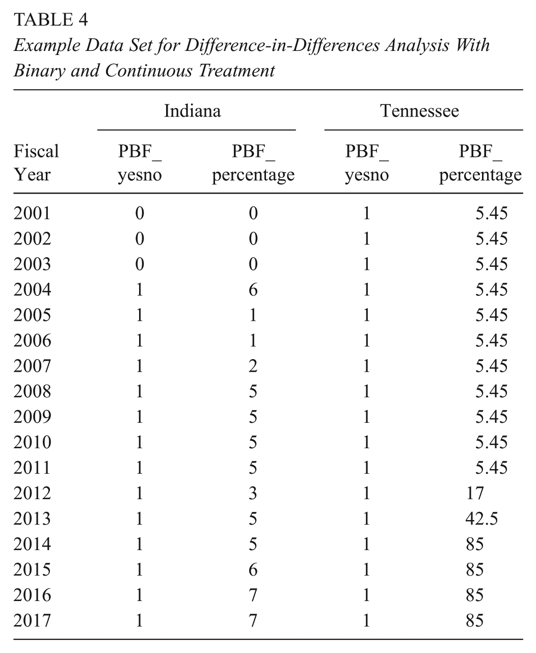
Example Data Set for Difference-in-Differences Analysis With Binary and Continuous Treatment

Fiscal Year	Indiana		Tennessee
Fiscal Year	PBF_yesno	PBF_percentage	PBF_yesno	PBF_percentage
2001	0	0	1	5.45
2002	0	0	1	5.45
2003	0	0	1	5.45
2004	1	6	1	5.45
2005	1	1	1	5.45
2006	1	1	1	5.45
2007	1	2	1	5.45
2008	1	5	1	5.45
2009	1	5	1	5.45
2010	1	5	1	5.45
2011	1	5	1	5.45
2012	1	3	1	17
2013	1	5	1	42.5
2014	1	5	1	85
2015	1	6	1	85
2016	1	7	1	85
2017	1	7	1	85

Recommendation 1: Set Internet search parameters to match how state legislative sessions and fiscal years align with academic years (modern search engines allow for searches to be limited to certain dates). Researchers who are interested in gathering data on policies as they were initially approved should use a search window that ends just after the beginning of an academic year, while those who are interested in the actual policy faced by an organization may wish to search through the end of the academic year. For example, when searching for PBF policies in place during the 2017–2018 academic year, we used October 1, 2016, to September 30, 2017, as our search dates for policies as approved by the legislature, and we extended that period to June 30, 2018, to examine policies as they were actually implemented.

Recommendation 2: Develop a range of terms to enter in search engines that would capture how different stakeholders talk about a policy. We use the term “performance-based funding” to talk about colleges that are funded in part based on outcomes, but a number of influential advocacy organizations have switched to the term “outcomes-based funding” in recent years (e.g., Lumina Foundation, n.d.; Miller & Morphew, 2017). To optimize data collection efforts, we use both of these terms in addition to “performance funding” and “outcomes funding” in conjunction with the words “higher education” (to limit the search results to relevant topics).

Recommendation 3: Use multiple search engines to make sure that all relevant results are collected. The optimal search engine to capture historical media coverage is LexisNexis, as that service has digitized many newspapers and magazines. We also used Google to research the details of a state’s PBF policy, but other Internet search engines are also suitable. One concern with most search engines is that they only return results for materials that are either currently online or were online in the past several weeks. This results in weaker coverage for older years, particularly when a state education agency replaces older materials with newer materials online. But in some cases, state education agency documents include multiple years of data, which may allow a look back into previous years (although such documents likely include final policy or funding decisions instead of what was initially promised to districts, schools, or colleges).

Recommendation 4: The Internet Archive: Wayback Machine (http://archive.org/web/) can be a valuable tool for researchers searching for information that was once online but has since been removed or modified. For example, as of January 2019, the Indiana Commission for Higher Education’s webpage on performance funding was at https://www.in.gov/che/3148.htm. The Wayback Machine archived 27 different versions of the site between 2014 and early 2018 at https://web.archive.org/web/*/https://www.in.gov/che/3148.htm, and the 2014 version had historical details going back to the beginning of PBF in Fiscal Year 2004 that were unavailable on the most recent version of the website.

Recommendation 5: Another potentially useful way to collect state policy data that are no longer readily available on websites is to follow logical URL patterns to see if additional years of reports are available. If a report includes “2016” in the URL, researchers can try to change the URL to “2015” to see if a prior year’s report is still available. This may only work in a small percentage of cases, but it can help fill in some gaps in the data.

Recommendation 6: Researchers who wish to collect data on state educational policies should work to develop relationships with state educational agencies before beginning to collect data. Organizations such as Education Commission of the States, the National Association of State Boards of Education, and the State Higher Education Executive Officers are excellent resources and can help facilitate conversations with individual states’ education agencies. Sharing the data collection strategy with several states’ officials can provide information on both the value of the proposed data set to policy makers (see Polikoff & Conaway, 2018, for a more detailed discussion of the importance of including practitioners in identifying the value of particular policy questions) and whether the data collection process is likely to pick up the desired elements. If an association feels the resulting data set will benefit its members, it may be willing to help researchers make connections with state agencies—a crucial tool for helping complete the data set.

After going through the above steps, a researcher can now begin collecting data. Rather than collecting data for one year or one state at a time, we strongly recommend that researchers collect data from a random sample of states for a random sample of years (with an oversample of earlier years of the data set) to make sure that the desired data elements can be collected. For large-scale data collection processes that involve a team of researchers (as well as graduate students), concerns regarding interrater reliability should be addressed. Multiple coders should independently code several state/year combinations to see if they all arrive at the same values. If coders disagree on more than a small percentage of observations, researchers should consider changing the data collection guidelines and/or providing additional training in order to increase the likelihood of coders agreeing. Once data collection for a state has been completed by one researcher, another researcher can independently collect and record information on the same data elements to ensure interrater reliability. Any discrepancies can be discussed as a research team and, in some cases, individual researchers can contact state education agencies for further clarification. As researchers learn more about the particular aspects of policies during the data collection process, additional elements that may need to be collected can be identified and the data dictionary and protocol can be updated appropriately.

Accounting for Policy Details in Difference-in-Differences Analyses

With educational policies being adopted and implemented in different ways across states, districts, schools, and colleges, more nuanced evaluations are increasingly important to understand the context in which policies are effective. While quasi-experimental designs can support continuous treatment variables, it is still relatively uncommon to do this in practice (Imbens & Wooldridge, 2009; St. Clair & Cook, 2015) due, at least in part, to the time-intensive nature of collecting and documenting detailed policy data and a small number of exemplars in education research on how to use continuous treatment variables. This leaves researchers with limited practical suggestions for incorporating continuous treatments into multistate policy evaluations, and the alternative of doing a series of individual analyses with each adopting state as a separate treatment group is often inefficient and insufficient as a way to influence discussions surrounding the efficacy of complex educational policies.

In this section, we demonstrate how researchers can use continuous treatment variables in quasi-experimental designs to support more detailed analyses of educational policies. We focus on DD designs since this method is frequently used to examine the impact of state educational policies, including PBF policies (e.g., Hillman et al., 2018; Hillman, Tandberg, & Gross, 2014; Tandberg, Hillman, & Barakat, 2014; Umbricht et al., 2017). Additionally, this section focuses on analyses at the state level to reflect on how policies may vary across states and within states over time. Analysts interested in sector-level or substate-level analyses (e.g., school, district, college, or student level) can use the same general DD framework by disaggregating data to an appropriate level, with the correct level to use varying across research questions and depending on whether different schools or colleges in a state were treated differently by a policy.

We provide a practical guide for how to conduct and interpret results from a DD analysis using a continuous rather than binary treatment variable and then discuss strategies to test assumptions underlying the DD model, drawing throughout on the PBF example described in the previous section. Table 5 provides examples of DD studies in education that use continuous treatment variables in policy evaluations, and we recommend Wing, Simon, and Bello-Gomez (2018) for a comprehensive—yet accessible—review of the DD method.

Table 5

Examples of Education Studies Using Difference-in-Differences Designs With Continuous Treatments

Study	Policy context	Treatment	Outcomes
Baird, Kofoed, Miller, and Wenger (2018)	Post 9-11 GI Bill changes	Dollar amount change in maximum benefit	Tuition at for-profit higher education institutions
Carruthers and Fox (2016)	Knox Achieves (college coaching and financial aid program in Tennessee)	Share of high school’s senior class participating in program	High school graduation, college enrollment, and college persistence
Domina, McEachin, Penner, and Penner (2015)	California’s Algebra for All effort	Changes in eighth grade algebra enrollment rates	10th grade mathematics achievement
Gershenson and Tekin (2018)	Beltway sniper attacks	Distance from traumatic event	School-level proficiency rates
Lucas (2010)	Malaria eradication campaigns in Paraguay and Sri Lanka	Changes in malaria infection rates	Female educational attainment
Lucas and Mbiti (2012a, 2012b)	Kenyan free primary education program	Percentage increase in primary school completers based on preprogram rates	Primary school participation, completion, and achievement
Shores and Steinberg (2017)	Great Recession	School district-level recession intensity and length of time exposed to recession	Student achievement

Conceptualizing DD Models With a Continuous Treatment Variable

The simplified DD model with two time periods (one before and one after policy adoption) and two groups (one that adopts a policy and one that does not) can be expressed:

y_{i t} = β_{0} + β_{1} p o l i c y_{i} + β_{2} p o s t_{t} + β_{3} (p o l i c y_{i} * p o s t_{t}) + ϵ_{i t}

where $y_{i t}$ is the outcome variable; $p o l i c y_{i}$ is a binary variable equal to 1 for states (or districts, schools, colleges, or students in states) that ever adopt a specific educational policy, $p o s t_{t}$ is a binary variable equal to 1 in all postpolicy years, $p o l i c y_{i} * p o s t_{t}$ is an interaction that equals 1 if a state ever adopts a specific policy and year is a postpolicy year and indicates treatment, $β_{3}$ is the DD estimate, and $ϵ_{i t}$ is the error term.

However, the simple DD model is often insufficient for analyses across states (or other units of analysis) due to policy adoption occurring in different years in different states, which requires an extension or generalization of the simple DD model in Equation 1. The generalized model includes a treatment variable that is the interaction of the (usually) binary policy variable and postadoption time period ( $p o l i c y_{i} * p o s t_{t}$ in Equation 1), year fixed effects, and unit (e.g., state, district, school, college) fixed effects. Year fixed effects capture the postpolicy binary variable ( $p o s t_{t}$ in Equation 1) and account for common time trends in outcome variables; unit fixed effects capture the policy variable ( $p o l i c y_{i}$ in Equation 1) and account for time-invariant characteristics of states, districts, schools, or colleges that could shape outcomes. The generalized DD model provides flexibility in the duration of treatment, which allows a particular educational policy to be enacted at different times and to alter once in place, can be expressed as:

y_{i t} = β_{1} t r e a t m e n t_{i t} + γ_{i} + δ_{t} + ϵ_{i t}

where $y_{i t}$ is the outcome of interest, $β_{1} t r e a t m e n t_{i t}$ is the treatment variable equal to 1 for states (or districts, schools, colleges, or students in states) with a particular policy in place in a given year, $γ_{i}$ are unit fixed effects, $δ_{t}$ are year fixed effects, and $ϵ_{i t}$ is the error term. In Equations (1) and (2), state or local covariates can be added to (1) reduce unexplained variance in the model and generate more precise estimates and (2) adjust for confounders that could surreptitiously influence outcomes. Covariates can be collected by the researchers as described in the previous section or can come from existing data sets, such as those maintained by the National Center for Education Statistics or from the Correlates of State Policy project at Michigan State University (Jordan & Grossmann, 2017).

In many state education policy evaluations, the policy variable in both simple and generalized DD designs are treated as binary, indicating either the presence or absence of a policy, such as PBF in higher education. In such analyses, any state that directs any funding to colleges based on performance metrics meets the PBF policy threshold and would be coded as 1. Similarly, in a substate analysis, any college (or college student) in a state that directs funds based on performance would be coded as 1. To examine differences in dosage in a DD framework, the binary policy treatment variable (labeled $p o l i c y_{i}$ in Equation 1 and $t r e a t m e n t_{i t}$ in Equation 2) can be replaced with a continuous policy treatment variable indicating a policy’s dosage as represented by the level or percentage of higher education funds tied to performance metrics.

Table 4 provides an example from our PBF data set that includes both a binary and continuous treatment variable for two states. The first state, Indiana, adopted a PBF policy in 2003. If treated as a binary variable, values in the “PBF_yesno” column take on 0 in prepolicy years (prior to 2003) and 1 in postpolicy years (2003 and later). If treated as a continuous variable, prepolicy years in which PBF was not yet in place would be coded as 0 in the same as in the binary case, as seen in the “PBF_percentage” column in years prior to 2003. Treatment in postpolicy years varied from year to year after PBF policy implementation, with the percentage of funds tied to outcomes ranging from 1% in 2004 and 2005 to 7% in 2014 and 2015. Tennessee’s PBF system, on the other hand, has been around since 1979, and the “PBF_yesno” variable is equal to 1 in all years. However, the percentage of funds tied to student outcomes increased sharply from just over 5% prior to 2010 to 85% in recent years.

Interpreting Results From DD Analyses With a Continuous Treatment Variable

In the case of a binary treatment variable, the DD coefficient can be interpreted as an intercept change or shift in the outcome of interest (e.g., degree production) after the introduction of a particular policy (e.g., PBF) in adopting states. However, with a continuous treatment variable, such as the share or amount of state higher education funding allocated based on student outcomes, the interpretation of the DD coefficient changes. The coefficient for the continuous treatment variable estimates whether colleges in states with a higher dosage policy (for instance, a larger share of funds tied to performance) experience larger impacts on outcomes. Specifically, the DD coefficient can be interpreted as a beta change in the outcome that is associated with a one-unit change in policy intensity conditional on the covariates.

One of the primary challenges associated with continuous treatment variables in education research is interpreting what the change in dosage level means from a practical perspective. In a binary treatment case, the change in treatment status is clear: schools, districts, or colleges are either subject to a policy or not, and the estimated effect is the impact of policy adoption on the specified outcomes. But in a continuous treatment case, changes in the dosage of a policy may not immediately provide practical advice for policy makers seeking to draft effective legislation, as policy makers are unlikely to focus debates on differences of 1 percentage point when drafting legislation.

Additionally, because a 1 percentage point change is small, the impact of this change on the outcome of interest is also likely to be small and difficult to interpret in a practical sense. Researchers could translate findings into a more meaningful change, such as a 5 or 10 percentage point change in the percent of funds tied to student outcomes in order to provide practical guidance for policy makers. Researchers could also interpret findings at various points in the distribution of existing policy designs—for instance, the impact on outcomes when dosage is set at the 25th and 75th percentiles—which can make findings more relevant for policy makers seeking to adopt policies with higher or lower levels of dosage.

Another way for researchers to examine the dosage or intensity of a policy is to create multiple discrete categories of state policies, such as “low,” “medium,” or “high” intensity adopting states based on the policy’s dosage. This may be particularly helpful if there are clear distinctions between policies in which there is a group of states that tie very small shares of funds to student outcomes (low intensity), a group that ties around half of funds to student outcomes (medium intensity), and another group that ties nearly all funding to student outcomes (high intensity). This specification allows researchers to examine whether the relationship between policy dosage and outcomes is nonlinear (i.e., the impact on outcomes varies depending on the level of policy intensity).¹

Researchers would need to examine the distribution of states within each grouping to determine whether the cut points for categories are appropriate. For instance, if there is a clustering of low-intensity states (e.g., less than 10% of funds tied to performance) while relatively few states attach the majority of funding to performance, the unbalanced distribution of states could create complications for the researcher. In such cases, estimating separate models using both continuous and discrete categorical treatment variables would be a good robustness check to determine whether results hold across both specifications. Examples of this particular strategy can be found in an economics study examining minimum wage changes (Card, 1992) and an education study examining the effect of community traumatic events on student achievement (Gershenson & Tekin, 2018). Additional technical considerations can be found in Imbens and Wooldridge (2009).

Finally, it is possible in a DD design to estimate the effects of multiple design elements of a policy at one time. In the case of PBF, for instance, researchers might be interested in how design elements of PBF policies relating to both institutional performance (e.g., percent of funds tied to degree completion) and specific equity metrics (e.g., percent of funds tied to enrollment and/or graduation of at-risk students) affect outcomes. Researchers can include separate terms for each of these elements in the model to better understand how various aspects of particular policies shape outcomes to inform many aspects of policy design.

Analyses that include continuous measures of a given educational policy are likely to be most useful when substantial variation in policy design exists. In some cases, the difference between the presence or absence of a policy might absorb any variation due to marginal shifts in a continuous aspect of the policy, especially if there is not substantial variation in the continuous measure. Researchers can include both the dichotomous policy adoption variable and the continuous dosage term for some particular aspect of a policy in the model at the same time to examine whether specific design aspects of a policy affect outcomes above and beyond the presence of the policy itself.

Testing Assumptions of the DD Model With a Continuous Treatment Variable

The primary identifying assumption underlying the DD model is that outcomes in adopting and nonadopting states would have followed parallel paths over time in the absence of policy adoption (Angrist & Pischke, 2008). Under this assumption, the differences in outcomes between treated and nontreated groups are constant in the pretreatment time period. For instance, states might adopt a policy based on trends in the outcomes of interest: for instance, if graduate rates at public institutions have fallen in recent years, legislators in that state may implement PBF in an effort to incentivize colleges to improve completion outcomes. If trends in outcomes, such as graduation rates, followed different trends over time in adopting and nonadopting states, any estimates from a DD model will reflect not only changes due to the policy but also different trends across states, resulting in biased estimates. This assumption is critical for identification in a DD design regardless of whether the policy being evaluated is treated as binary or continuous. The same identifying assumption also holds in the case of a continuous variable because dosage may not be exogenous: for instance, states with steeper declines in graduation rates may implement PBF policies tying larger shares of funds to outcomes in order to provide stronger incentives for institutions to improve performance.

In a relatively simple DD model when policy adoption occurs at one time period but multiple prepolicy years are observed, researchers can visually examine outcomes for prepolicy trends, plotting means for adopting and nonadopting states in years leading up to policy adoption. This method becomes more complicated to apply when adoption occurs at different time periods or when the policy is measured as a continuous variable rather than binary. Visual examinations of prepolicy trends become even more difficult to do if states change the dosage or intensity of a policy over time, as described in the Tennessee example above. In such cases, there is not a clear “treatment” and “comparison” group to use to examine parallel trends in years leading up to policy adoption but rather different levels of treatment each year after policy adoption (and for each treated state). One option is for researchers to provide graphical depictions of trends in outcomes over time when (1) treatment is considered binary (PBF-adopting vs. PBF nonadopting states) or (2) treatment is considered as multiple discrete categories (e.g., high, medium, and low PBF intensity states). Although visualizations of prepolicy trends do not offer a formal statistical test of the parallel trend assumption, we still recommend researchers provide this visualization in some form when treatment is measured continuously.

One strategy to test for parallel trends for both continuous and binary policies is to conduct a modified Granger causality test, assigning leads for policy adoption (often in each year up to 3–5 years prior to actual adoption) and estimating Equation (2). The coefficients for leads in this falsification test—that is, when policy adoption is set to occur prior to years when it was actually in place—should not be significant. In other words, there should not be any effect of the policy on outcomes of interest in years prior to actual policy adoption. If coefficients on the lead variables are significant, the parallel trends assumption may be violated. Researchers can also include lagged treatment variables in the model to examine whether there is a delayed response to a policy (or to a change in the dosage of a policy). For instance, a lagged response would surface if colleges were slow to respond to PBF incentives and the impact of the policy increased (or decreased) over time. Statistical software programs, such as Stata, allow leads and lags for continuous variables in the same way they do for binary variables.

A second strategy that can be used with both binary and continuous treatment variables (but that becomes even more important given the difficulty visualizing pretreatment trends in the latter case) is to relax the parallel trend assumption and allow each state, school, district, or college to have a unique time trend. To do this, researchers interact a continuous time variable with a dummy variable for each unit of analysis (state, school, district, or college) and estimate a model with the inclusion of this unit-specific time trend. Researchers then examine the robustness of the findings to this specification to determine whether results are consistent when the parallel trend assumption is relaxed and each unit is allowed to follow a unique trend over time. If results are consistent across the two specifications, there would appear to be more support for parallel trends.²

Conclusion

As states lead the way in adopting (and repeatedly changing) a range of educational policies in an effort to improve student outcomes, the traditional analytic strategy of policy evaluation based on the simple absence or presence of a policy is being viewed with increased skepticism from different stakeholders. As top-tier academic journals increasingly demand more nuanced evaluation strategies while policy makers and advocacy groups push back against analyses that do not account for a given state’s peculiar characteristics researchers are being pushed toward conducting more detailed analyses of state policies. This development allows for inferences to be drawn regarding the extent to which dosage and particular design characteristics matter among states that have adopted different variations of the same policy (such as the PBF example used throughout this article).

In this article, we provided strategies for researchers who seek to compile detailed state-level and institutional-level data sets to better understand the impacts that educational policies can have on both students and institutions. However, we also recognize that these types of data collection efforts can be incredibly time consuming for researchers. Our PBF data set will take 2 years to be fully constructed and checked by a team of three faculty members and two graduate students. Although it would have been far faster to construct a binary data set indicating whether states had any PBF system in a given year, we strongly believe that the upfront investment of building a comprehensive data set will pay off in the long run via greater research and policy relevance. We also provide guidance for how to conduct DD analyses when treatment is measured as a continuous variable, in particular discussing how to interpret results and draw meaningful conclusions for policy makers as well as offer suggestions for testing the assumptions of the model in the case of a continuous treatment variable.

Both nonacademic and academic audiences have a role to play in encouraging more researchers to invest large amounts of time and resources in building better data sets and conducting detailed analyses using these data. Foundations and policy organizations alike can help by making resources available to support data collection and cleaning efforts. These organizations often prefer to support low-cost analyses of existing data sets or randomized trials, but we argue that digging into the nuanced details of educational policies allows for researchers to study policies as they were actually implemented instead of simply whether they were enacted.

Academic institutions should also provide incentives for researchers to compile state-level policy data sets; otherwise, graduate students and pretenure faculty members may see the time costs of these projects as exceeding the benefits of the resulting papers. In order for academics to be incentivized to construct the types of comprehensives data sets described in this article, peer-reviewed journals must recognize the act of building a data set as a significant contribution to the body of knowledge, while hiring and tenure/promotion committees would need to be aware of the difficulty of creating a data set from scratch instead of relying on publicly available data sources. The academic community at large would also need to reward the outcomes of the data collection process, giving credit to researchers when their data set helps influence educational policies and state legislation.

Finally, we strongly encourage researchers to make their data publicly available after conducting initial analyses (in order to make sure that those who collected the data have the first opportunity to publish findings using those data). Efforts by Sean Reardon to compile data on racial/ethnic segregation and test score gaps in K–12 education, the Opportunity Insights Project to examine social mobility rates in higher education, and PennAHEAD’s detailed database of college Promise program features are three excellent examples for future researchers to follow (Chetty, Friedman, Saez, Turner, & Yagan, 2017; Perna & Leigh, 2018; Reardon, 2016). Both of these data releases came with substantial media attention that further highlighted their published research and allowed their findings to reach more state education policy makers, and we will be making our initial data set available to the public in 2020. Future researchers who decide to make their data set publicly available would also allow other researchers to cite and replicate the data set as well as expand on previous analyses and data collection, increasing its value in the academic labor market.

Footnotes

Acknowledgements

We are grateful to the William T. Grant Foundation for supporting our data collection efforts. We would also like to thank Lynneah Brown, Karly Caples, and Nicholas Voorhees for their efforts in compiling our data set on state performance-based funding policies.

ORCID iD

Justin C. Ortagus

Notes

Authors

ROBERT KELCHEN is an associate professor in the Department of Education Leadership, Management and Policy at Seton Hall University. His research interests include higher education finance, accountability policies and practices, and student financial aid.

KELLY OCHS ROSINGER is an assistant professor in the Department of Education Policy Studies and a research associate with the Center for the Study of Higher Education at Pennsylvania State University. Her research focuses on the barriers students face going to and through college and the impact of policies and interventions designed to improve college access and success.

JUSTIN C. ORTAGUS is an assistant professor of higher education and the director of the Institute of Higher Education at the University of Florida. His research examines how online education, community colleges, and various state policies affect the opportunities and outcomes of underserved students.

References

Angrist

J. D.

Pischke

J. S.

(2008). Mostly harmless econometrics: An empiricist’s companion. Princeton, NJ: Princeton University Press.

Baird

Kofoed

Miller

Wenger

(2018). For-profit higher education responsiveness to price shocks: An investigation of changes in post 9-11 GI Bill allowed maximum tuitions. Retrieved from https://papers.ssrn.com/sol3/papers.cfm?abstract_id=3174763

Card

(1992). Using regional variation in wages to measure the effects of the federal minimum wage. ILR Review, 46, 22–37.

Card

Payne

A. A.

(2002). School finance reform, the distribution of school spending, and the distribution of student test scores. Journal of Public Economics, 83, 49–82.

Carruthers

C. K.

Fox

W. F.

(2016). Aid for all: College coaching, financial aid, and post-secondary persistence in Tennessee. Economics of Education Review, 51, 97–112.

Chetty

Friedman

J. N.

Saez

Turner

Yagan

(2017, July). Mobility report cards: The role of colleges in intergenerational mobility (Working Paper 23618). Cambridge, MA: National Bureau of Economic Research.

Dillon

(2011, September 23). Obama turns some powers of education back to states. The New York Times. Retrieved from https://www.nytimes.com/2011/09/24/education/24educ.html

Domina

McEachin

Penner

(2015). Aiming high and falling short: California’s eighth-grade algebra-for-all effort. Educational Evaluation and Policy Analysis, 37, 275–295.

Dougherty

K. J.

Natow

R. S.

(2015). The politics of performance funding for higher education: Origins, discontinuations, and transformations. Baltimore, MD: Johns Hopkins University Press.

10.

Dougherty

K. J.

Natow

R. S.

Pheatt

Reddy

(2016). Performance funding for higher education. Baltimore, MD: Johns Hopkins University Press.

11.

Doyle

W. R.

(2010). Does merit-based aid “crowd out” need-based aid? Research in Higher Education, 51, 397–415.

12.

Elazar

(1972). American federalism. New York, NY: Thomas Crowell.

13.

Fain

(2018, May 9). Plans for performance funding for Calif.’s 2-year colleges. Inside Higher Ed. Retrieved from https://www.insidehighered.com/quicktakes/2018/05/09/plans-performance-funding-califs-2-year-colleges

14.

Finger

L. K.

(2018). Vested interests and the diffusion of education reform across the states. Policy Studies Journal, 46, 378–401.

15.

Fitzpatrick

M. D.

Jones

(2016). Post-baccalaureate migration and merit-based scholarships. Economics of Education Review, 54, 155–172.

16.

Gándara

Rutherford

(2018). Mitigating unintended impacts? The effects of premiums for underserved populations in performance-funding policies for higher education. Research in Higher Education, 59, 681–703.

17.

Gershenson

Tekin

(2018). The effect of community traumatic events on student achievement: Evidence from the Beltway Sniper attacks. Education Finance and Policy, 13, 513–544.

18.

Hanushek

E. A.

Raymond

M. E.

(2005). Does school accountability lead to improved student performance? Journal of Policy Analysis and Management, 24, 297–327.

19.

Hearn

J. C.

McLendon

M. K.

Linthicum

K. C.

(2017). Conceptualizing state policy adoption and diffusion. In Paulsen

M. B.

(Ed.), Higher education: Handbook of theory and research (Vol. 32, pp. 309–354). Dordrecht, Netherlands: Springer.

20.

Hillman

N. W.

Fryar

A. H.

Crespín-Trujillo

(2018). Evaluating the impact of performance funding in Ohio and Tennessee. American Educational Research Journal, 55, 144–170.

21.

Hillman

N. W.

Tandberg

D. A.

Fryar

A. H.

(2015). Evaluating the impacts of “new” performance funding in higher education. Educational Evaluation and Policy Analysis, 37, 501–519.

22.

Hillman

N. W.

Tandberg

D. A.

Gross

J. P.

(2014). Performance funding in higher education: Do financial incentives impact college completions? Journal of Higher Education, 85, 826–857.

23.

Imbens

G. W.

Wooldridge

J. M.

(2009). Recent developments in the econometrics of program evaluation. Journal of Economic Literature, 47, 5–86.

24.

Jackson

C. K.

Johnson

R. C.

Persico

(2016). The effects of school spending on educational and economic outcomes: Evidence from school finance reforms. Quarterly Journal of Economics, 131, 157–218.

25.

Jones

Elliott

Owens

Assalone

Gándara

(2017). Outcomes based funding and race in higher education. Cham, Switzerland: Palgrave Macmillan.

26.

Jordan

M. P.

Grossmann

(2017). The Correlates of State Policy Project v.2.1. Retrieved from http://ippsr.msu.edu/public-policy/correlates-state-policy

27.

Karch

(2007). Democratic laboratories: Policy diffusion among the American states. Ann Arbor: University of Michigan Press.

28.

Kelchen

(2018a). Do performance-based funding policies affect underrepresented student enrollment? Journal of Higher Education, 89, 702–727.

29.

Kelchen

(2018b). Higher education accountability. Baltimore, MD: Johns Hopkins University Press.

30.

Kelchen

Stedrak

L. J.

(2016). Does performance-based funding affect colleges’ financial priorities? Journal of Education Finance, 41, 302–321.

31.

Klein

(2016, January 5). Under ESSA, states, districts to share more power. Education Week. Retrieved from https://www.edweek.org/ew/articles/2016/01/06/under-essa-states-districts-to-share-more.html

32.

Kramer

D. A.

II Ortagus

J. C.

Lacy

T. A.

(2018). Tuition-setting authority and broad-based merit aid: The effect of policy intersection on pricing strategies. Research in Higher Education, 59, 489–518.

33.

Krane

(2007). The middle tier in American federalism: State government policy activism during the Bush presidency. Publius, 37, 453–477.

34.

Lacy

T. A.

Tandberg

D. A.

(2014). Rethinking policy diffusion: The interstate spread of “finance innovations.” Research in Higher Education, 55, 627–649.

35.

A. Y.

(2018). In high demand: Performance funding policy impacts on STEM degree attainment. Educational Policy. Advance online publication. doi:10.1177/0895904818755455

36.

Lucas

A. M.

(2010). Malaria eradication and educational attainment: Evidence from Paraguay and Sri Lanka. American Economic Journal: Applied Economics, 2(2), 46–71.

37.

Lucas

A. M.

Mbiti

I. M.

(2012a). Access, sorting, and achievement: The short-run effects of free primary education in Kenya. American Economic Journal: Applied Economics, 4(4), 226–253.

38.

Lucas

A. M.

Mbiti

I. M.

(2012b). Does free primary education narrow gender differences in schooling? Evidence from Kenya. Journal of African Economies, 21, 691–722.

39.

Lumina Foundation. (n.d.). Frequently asked questions outcomes-based funding. Retrieved from https://www.luminafoundation.org/outcomes-based-funding-faq

40.

McDermott

K. A.

(2003). What causes variation in states’ accountability policies? Peabody Journal of Education, 78(4), 153–176.

41.

Miller

G. N. S.

Morphew

C. C.

(2017). Merchants of optimism: Agenda-setting organizations and the framing of performance-based funding for higher education. Journal of Higher Education, 88, 754–784.

42.

Mintrom

(1997). The state-local nexus in policy innovation diffusion: The case of school choice. Publius, 27(3), 41–59.

43.

Mississippi Institutions of Higher Education. (2013). Performance allocation model summary. Retrieved from www.mississippi.edu/downloads/ihl_130418-2.pdf

44.

Mokher

C. G.

McLendon

M. K.

(2009). Uniting secondary and postsecondary education: An event history analysis of state adoption of dual enrollment policies. American Journal of Education, 115, 249–277.

45.

National Association of State Budget Officers. (2018). The fiscal survey of states: Spring 2018. Washington, DC: Author.

46.

National Conference of State Legislatures. (2015). Performance-based funding for higher education. Retrieved from https://web.archive.org/web/20180709174718/http://www.ncsl.org/research/education/performance-funding.aspx

47.

Perna

L. W.

Leigh

E. W.

(2018). Understanding the promise: A typology of state and local college promise programs. Educational Researcher, 47, 155–180.

48.

Polikoff

Conaway

(2018, September 25). Getting beyond “did it work?”: Proposing a new approach to integrate research and policy. Retrieved from https://www.brookings.edu/blog/brown-center-chalkboard/2018/09/25/getting-beyond-did-it-work-proposing-a-new-approach-to-integrate-research-and-policy/

49.

Reardon

S. F.

(2016). School segregation and racial academic achievement gaps. RSF: The Russell Sage Foundation Journal of the Social Sciences, 2(5), 34–57.

50.

Shores

Steinberg

(2017). The impact of the Great Recession on student achievement: Evidence from population data. Retrieved from https://papers.ssrn.com/sol3/papers.cfm?abstract_id=3026151

51.

Sjoquist

D. L.

Winters

J. V.

(2015). State merit aid programs and college major: A focus on STEM. Journal of Labor Economics, 33, 973–1006.

52.

Snyder

Boelscher

(2018). Driving better outcomes: Fiscal year 2018 state status & typology update. Washington, DC: HCM Strategists.

53.

Snyder

Fox

(2016). Driving better outcomes: Fiscal year 2016 state status & typology update. Washington, DC: HCM Strategists.

54.

Springer

M. G.

(2008). The influence of an NCLB accountability plan on the distribution of student test score gains. Economics of Education Review, 27, 556–563.

55.

St. Clair

Cook

T. D

. (2015). Difference-in-differences methods in public finance. National Tax Journal, 68, 319–338.

56.

Tandberg

D. A.

Hillman

Barakat

(2014). State higher education performance funding for community colleges: Diverse effects and policy implications. Teachers College Record, 116(12), 1–31.

57.

Umbricht

M. R.

Fernandez

Ortagus

J. C.

(2017). An examination of the (un)intended consequences of performance funding in higher education. Educational Policy, 31, 643–673.

58.

Wing

Simon

Bello-Gomez

R. A.

(2018). Designing difference in difference studies: Best practices for public health policy research. Annual Review of Public Health, 39, 453–469.

59.

Wong

K. K.

Shen

F. X.

(2002). Politics of state-led reform in education: Market competition and electoral dynamics. Educational Policy, 16, 161–192.

60.

Wong

V. C.

Wing

Martin

Krishnamachari

(2018). Did states use implementation discretion to reduce the stringency of NCLB? Evidence from a database of state regulations. Educational Researcher, 47, 9–33.

How to Create and Use State-Level Policy Data Sets in Education Research

Abstract

Keywords

Case Study: Performance-Based Funding in Higher Education

Constructing a State Policy Data Set

Accounting for Policy Details in Difference-in-Differences Analyses

Conceptualizing DD Models With a Continuous Treatment Variable

Interpreting Results From DD Analyses With a Continuous Treatment Variable

Testing Assumptions of the DD Model With a Continuous Treatment Variable

Conclusion

Footnotes

Acknowledgements

ORCID iD

Notes

Authors

References