Sage Journals: Discover world-class research

Abstract

In an era of increased accountability for colleges and concerns about an affordable education, it is useful to understand whether students can adequately manage the debt burden they hold after leaving higher education. In 2015, Texas called for cumulative undergraduate debt to be 60% or less of public institution graduates’ first-year earnings by 2030. I investigate the student-level characteristics that are associated with a debt-to-income ratio above 60%. The data come from five cohorts of undergraduate students who attended Texas public 4-year institutions. I find that if sanctions were attached to the cumulative debt goal, historically disadvantaged groups of students and institutions that serve these students likely would be disproportionately affected by this type of accountability goal even after controlling for prior income, parental education, major choice, and time to degree. Policy implications are discussed.

Keywords

colleges correlational analysis diversity educational policy

In recent decades, the number of students using federal loans to finance their undergraduate careers has increased, though the average amount of federal debt per student has been relatively stable in constant dollars (Avery & Turner, 2012; College Board, 2015). Still, the variation in the amount of debt per student has increased over time (College Board, 2014), signaling the potential for financial inequities among college student subgroups if the variation is not evenly distributed. In response to a growing concern about these financial inequities and what they mean for student attainment and later-life outcomes, a small but rapidly growing number of states and institutions have begun implementing policies aimed at containing or capping the amount of student debt that students accumulate (Urban Institute, 2017).

The federal government has a number of ways it can hold institutions accountable for the debt burden of students (see Kelchen, 2018b, for an overview). However, states have generally focused on: (a) tying an amount of an institution’s state appropriations to the institution’s success at attaining certain outcomes, such as reaching a set number of certificates and degrees conferred (performance- or outcomes-based funding; Kelchen, 2018b), or (b) capping or freezing the increase in an institution’s tuition or fees (Kelchen & Pingel, 2018). The primary focus of these performance-based funding models is rarely the debt burden of graduates. To my knowledge, two states include some direct measure of college affordability or debt in their performance-based funding model (National Conference of State Legislatures [NCSL], 2015; University of Wisconsin System, 2017). These are relatively new changes. Vermont is transitioning to this funding formula (NCSL, 2015),¹ and Wisconsin approved the change in December of 2017 (University of Wisconsin System, 2017). Both states propose to assess the average student loan debt upon conferral of a credential. Neither state has any measure of the income or earnings of students after receipt of their credential. Further, in academic year 2016–2017, 27 of 44 states responding to a survey reported either freezing tuition or limiting the amount an institution could increase the tuition (Kelchen, 2017). Tuition freezes or caps can be controversial, particularly as research finds that these policy tools rarely curb student loan debt or the overall price for students (Kim & Ko, 2015).

To focus on increasing college affordability, the state of Texas created a new measure of student debt burden and included that measure in its 2030 strategic plan, 60x30TX (Texas Higher Education Coordinating Board [THECB], 2015). The strategic plan has a primary motivation to increase state postsecondary attainment levels, but one of its four key goals includes a specific focus on the affordability of higher education for students once they have completed their credential (THECB, 2015).² In the strategic plan, Texas calls for cumulative undergraduate debt to be 60% or less of public institution graduates’ first-year earnings by 2030 (referred to as the Texas debt burden cap goal, or DBCG, for the rest of the article; THECB, 2015). For example, if a student borrowed $30,000 in undergraduate student loans and had a salary of $50,000 the year after graduating from college, the student would have a 60% debt-to-income ratio. This is the state of Texas’s indicator of repayment concerns. Research shows that students who default or struggle with repayment of their student loans often are not the students with the highest student loan balances (e.g., Woo, Bentz, Lew, Smith, & Velez, 2017). If students with higher loan balances also obtain occupations with higher salaries, the loan repayment process could be manageable.

Prior research (see Hillman, 2015, for an overview) has focused on the ways individual and institutional characteristics are associated with the average amount of debt students accumulated. This is only one part of the picture. The characteristics that influence a student to borrow an average amount of undergraduate debt may be different than those that influence the student borrowing a small or large amount of debt. Also, the Texas threshold of 60% is determined by the historical data on the median undergraduate student debt relative to earnings. Texas and other states considering this type of policy or strategic goal prefer to use the median instead of the mean to mitigate the effect of extremely small or large debt-to-income ratios.

With these trends in college borrowing in mind, I use unconditional quantile regression to investigate:

Research Question 1: To what extent are student-level characteristics associated with the distribution of cumulative undergraduate debt more generally?

Research Question 2: To what extent are student-level characteristics associated with the distribution of the ratio of cumulative undergraduate debt to first-year income more generally?

There is not enough data on years since the introduction of the DBCG to investigate the effect of the actual goal.³ However, it is critical when hypothesizing the potential effects of the DBCG to better understand Texas undergraduate students’ trends in borrowing and earning behaviors. Evidence from these research questions is useful for policymakers and researchers across the United States. For policy stakeholders, the current study provides evidence on the potential unintended consequences of an accountability goal like the DBCG, which are critical to understand when designing and implementing a statewide goal for college affordability. For example, if institutions with more underserved students have consistently high debt-to-income ratios, policy stakeholders may need to be wary of tying sanctions to institutions or individuals without taking that into consideration. For researchers, the current study provides additional evidence on the relationship between college affordability and student-level characteristics (particularly by modeling this relationship with a focus beyond the average student).

As an example of the usefulness in studying the entire distribution of debt-to-income, I posit a relationship between race and debt-to-income ratios. When including an indicator of whether students are Latinx in an ordinary least square (OLS) regression, the students are compared to their White peers (or another reference group) in the average amount of debt-to-income ratio. While this would be informative, it could be that the relationship between race (more specifically, structures and experiences associated with race since race is socially constructed) and debt-to-income ratio differs based on where in the distribution of the ratio one is interested. For example, at the average debt-to-income ratio, Latinx students may be predicted to have a smaller debt-to-income ratio than their White peers (whether due to earning more or borrowing less). However, when investigating this relationship across the distribution of debt-to-income ratios, at larger ratios (e.g., 80th percentile of debt-to-ratio), quantile regression could show that Latinx students actually are predicted to have higher debt-to-income ratios than their White peers.

Using OLS, one would assume that Latinx students have smaller predicted debt-to-income ratios than their White peers and may not need to be the target of any policies to create structures to help these students manage their debt burden. But, if state policymakers are concerned about students with larger debt-to-income ratios, then Latinx students are actually one of the key groups of students the policymakers would need to be concerned about for debt burden management. These types of nuances in relationships can be discovered using unconditional quantile regression.

While the state of Texas has one of the most robust state administrative databases, there are constraints to policies or strategic goals crafted to use this type of data. For example, due to the state’s inability to access repayment information for residents, the DBCG does not take into account the student loan repayment plan that individuals select. Therefore, a student with an income-based repayment plan would be treated the same as a student with a standard repayment plan in Texas’s strategic plan (even though the two students likely have different monthly payments).⁴ Also, since Texas and any other state with this type of administrative database can only track the salary of individuals who reside within the state, any students who move outside of Texas cannot be included in the DBCG ratio measure. These constraints have implications for the utility of this type of institutional accountability measure (discussed in the discussion section).

The Texas DBCG also focuses solely on students who earn a credential. As will be discussed throughout the article, this creates a significant limitation in what the metric can and cannot tell state policymakers about college affordability and ability to repay. However, in general, without increased access to existing federal databases to track college students’ experience in the labor market, any state that wishes to create a similar higher education accountability tool will need to negotiate similar constraints. For this reason, the current study presents evidence on a potential new higher education accountability tool, debt-to-income ratios, while highlighting the potential constraints other states would face if creating a similar policy.

Literature Review

To better understand the characteristics associated with student debt-to-income ratio and the Texas DBCG, it becomes essential to outline (a) the evidence on student loan repayment and default and (b) the policy background of the DBCG in Texas.

Student Loan Repayment

Prior research shows that a student’s age, dependency status, income background, parental education, ability to complete a degree in a shorter time, race/ethnicity, and institutional price are all associated with how much they will borrow (Avery & Turner, 2012; Baum & O’Malley, 2003; College Board, 2015; Houle, 2013; Malcom & Dowd, 2012). Typically, the student loan debt burden of undergraduates at U.S. institutions is measured as the ratio of the students’ income to the students’ repayment amount (e.g., Chapman & Dearden, 2017). Generally, this is either calculated on a monthly or yearly basis. For example, federal gainful employment regulations calculate a debt-to-earnings ratio (different from the Texas debt-to-income ratio), which compares students’ annual student loan payment amount to either their discretionary or total annual income (Office of Postsecondary Education, 2014). However, when the amount students are expected to repay is unclear, scholars have used the total amount of student loans borrowed as a proxy for the repayment amount (THECB, 2015). For example, the goal of the DBCG is to maintain a sustainable undergraduate debt burden for graduates of Texas public institutions by comparing the graduates’ cumulative amount of undergraduate student loans to the first year of earnings, as further discussed in the Texas policy context section. The goal of finding the optimal amount of student loan debt burden for students is often to decrease the likelihood of loan default (failing to make a payment for over 270 days).

Some of the predictors of student loan default are: earnings after leaving higher education being low or nonexistent (due to unemployment), not earning a credential, identifying with an underrepresented racial/ethnic group, coming from a lower-income family, being older, or attending a for-profit institution (Belfield, 2013; Gross, Cekic, Hossler, & Hillman, 2009; Hillman, 2014; Looney & Yannelis, 2015; Price, 2004). For example, Looney and Yannelis (2015) analyzed data representing a random sample of all federal student borrowers in the National Student Loan Data System (approximately 4%) from 1970 to 2014; they merged these data with earnings and income data from tax information from 1999 to 2014. The general national trends in higher default rates in recent decades appeared to be driven by the larger numbers of nontraditional students entering higher education, who are more vulnerable to default. The authors also found that labor market characteristics, earnings, and income significantly contribute to the rise in student default from 2000 to 2011. This would mean that while defaulting on educational debt has been on the rise primarily for nontraditional students, the occupational earnings of students influenced the likelihood of students defaulting. This is one of the primary reasons it is essential when crafting accountability measures to not focus solely on students’ cumulative amount of student loans.

There is no clear consensus on the exact amount of debt burden that predicts a borrower’s difficulty with repayment. Some scholars and policy intermediary organizations have advocated for student loan payments to be 8% to 10% of students’ income (e.g., Price, 2004; Tandberg, Laderman, & Carlson, 2017). However, other research argues that when students’ repayment amount becomes 18% or more of the students’ income, it is likely that the students will have significant hardships with repaying their student loans (e.g., Baum & Schwartz, 2006; Chapman & Dearden, 2017). This range in the threshold for maximum debt-to-income ratios that are manageable (8%–18%) is the closest estimate available to compare for the DBCG measure of debt burden (a ratio of total undergraduate debt to the earnings of students). As Texas does not collect repayment information on student debt, the standard debt-to-income ratio (a ratio of student loan payment amount to income) cannot be calculated. However, a student in the analytical sample for the current study who was compliant with the DBCG, with an average amount of undergraduate debt, would have standard monthly payments that were approximately 7% of their monthly income.⁵ Therefore, the state of Texas’s threshold for DBCG actually creates a more conservative cutoff for the student with average debt than the scholarly and national policy community suggest for standard debt-to-income ratios.

Texas Policy Context

The state of Texas, with support from the THECB, estimates a debt-to-income ratio each year for every student graduating from a public institution. The ratio includes students’ undergraduate debt for the 15 years preceding earning either a certificate, associate’s degree, or bachelor’s degree and their earnings for 1 year after graduation (THECB, 2017). For the income portion of the ratio, the state includes any students who have earned a wage in at least three of four quarters in the year after earning a credential.⁶ This ratio does not include students who do not earn a credential. The THECB then calculates the median debt-to-income ratio of all the student debt-to-income ratios. This median estimate is the target of 60x30TX and the focus of the 60% maximum cutoff for public institutions. The Texas DBCG does not apply to private not-for-profit or for-profit institutions in Texas. The state proposes to maintain, at most, a 60% debt-to-income ratio by focusing on cutting the number of excess credit hours earned and keeping the percentage of students who borrow at 50% (THECB, 2015).⁷

The explicit focus on affordability, specifically, a debt-to-income ratio threshold, in Texas’s strategic plan is in part due to the potential negative consequences of overly large debt burdens both to the individual and society at large (Baker & Doyle, 2017; Malcom & Dowd, 2012; Rothstein & Rouse, 2011; THECB, 2015). National and state research shows that historically disadvantaged students, particularly those who identify as women, Black, or low income, borrow at the highest rates, borrow the largest amounts, and struggle the most with repayment (e.g., American Association of University Women, 2017; Hillman, 2015). While the average Texas student loan amount is below the national average (Fernandez, Fletcher, & Klepfer, 2016), 49% of borrowers had a subprime credit score, below 620, indicating repayment of student loans likely would be challenging (Di & Perlmeter, 2014). These concerns about the ability to repay undergraduate debt drove state higher education policymakers to create the DBCG. Currently, Texas does not attach any penalties to failing to meet the 60% threshold, nor does it estimate separate debt-to-income ratios for different institutions (Fernandez et al., 2016). This lack of penalty could shift depending on desires of the leadership of the state legislature and the THECB.

This case study of debt-to-income ratio in Texas improves both the scholarly understanding of debt and provides evidence for the creation and implementation of better targeted accountability tools in Texas and other states. Also, this case study broadens the national research evidence base on undergraduate debt and postcollege debt burden, which increases its usefulness beyond the state of Texas. In terms of applicability to other states, Texas is a relevant state for a case study for many reasons. Texas is near the national average of residents with at least a bachelor’s degree (THECB, 2016). Texas is also near the national average for tuition and fees, ranking 20th for public 4-year institutions and 30th for private 4-year institutions (THECB, 2016). Median household income was approximately $53,000 in 2014, ranking Texas number 23 nationally (THECB, 2016). This makes it likely that other states’ policymakers would find the results from research conducted on Texas data useful for their own contexts. Further, Texas has one of the most robust state administrative databases in the country (Kelchen, 2018b). The same data limitations that affect Texas state policymakers’ choices in creating debt-to-income policies for students will also affect other states with administrative databases.

Also, across the United States, concerns about college affordability and students’ ability to manage repayment have led other state policymakers to consider creating an accountability goal similar to Texas’s DBCG (J. Marsh, personal communication). Therefore, learning about the structures and implications of the Texas DBCG can help other states in crafting higher education accountability tools that focus on college affordability. It also provides more evidence on the types of students or institutions who would be disproportionately affected by similar accountability measures, which is critical as the other primary state accountability tool, performance-based funding, has been shown to potentially harm enrollments of students from historically disadvantaged populations (Gándara & Rutherford, 2018, McKinney & Hagedorn, 2017).

Another example of potential unintended harm is for so-called education triage (coined by Gillborn & Youdell, 2000), which was a hypothesized response from k–12 school systems after they introduced accountability testing and proficiency counts (Ballou & Springer, 2017; Neal & Schanzenbach, 2010). Neal and Schanzenbach (2010) found that Chicago Public School students in the middle of the achievement distribution, below but near the cutoff for a rating of proficiency, saw gains in academic achievement not replicated for students at the lower ends of the distribution. The authors and the popular press argued that certain schools may face “a strong incentive to shift attention away from their lowest-achieving students and toward students near proficiency” (Neal & Schanzenbach, 2010, p. 280). While other scholars (e.g., Ballou & Springer, 2017) were not able to replicate this finding, there are still concerns that creating arbitrary thresholds with sanctions, as attaching consequences to the Texas DBCG would do, shifts institutional energies to students nearest the threshold.

Method

Data

I use Texas state administrative data from the THECB to analyze the relationship between individual and institutional characteristics and the amount of undergraduate debt students accumulate as well as those students’ debt-to-income ratios.⁸ To investigate students’ debt-to-income ratio, I merge quarterly earnings data from the Texas Workforce Commission (TWC) with the THECB’s data on enrollment, graduation, and financial aid. Prior research primarily focuses on smaller samples or national, longitudinal data sets that irregularly follow students and do not include information on the earnings of students. To fully investigate borrowing and earning behaviors, the repository of linked financial aid records, postsecondary transcripts, and labor market information is critical.

The outcome measures are cumulative undergraduate debt of bachelor’s degree recipients (Research Question 1) and the debt-to-income ratios of those same students (Research Question 2). Undergraduate debt includes the following types of loans: Perkins loans, College Access Loan, Primary Care student loans, subsidized federal direct loans, unsubsidized federal direct loans, Be on Time loan, HB3015 loans, and other loans. When measuring total undergraduate debt including parent contributions, I also include federal Direct PLUS loans (often referred to as parent PLUS loans). Texas defines debt-to-income ratio as the ratio of the total cumulative debt (including parent PLUS loans) to annual earnings of graduates in their first year after earning either a certificate or associate’s or bachelor’s degree (THECB, 2015). Earnings data come from unemployment insurance information collected by the TWC; therefore, certain workers’ wages are not collected (e.g., self-employed). Following THECB practice, I only include earnings for students who had reported wages or salary income in at least three of the four quarters in the year. I include debt-to-income ratio as a percentage.

I define the analytical sample as student borrowers who earned a bachelor’s degree from a public institution and have both financial aid data from the THECB and earnings data from the TWC. I only include students who have borrowed since the state cannot calculate a debt-to-income ratio for nonborrowers. I focus on first-time bachelor’s degree earners to restrict the outcomes in the sample for students who earn both an associate’s degree and a bachelor’s degree.⁹ Due to availability of financial aid data (THECB did not begin consistently collecting this information until 2004), I focus on students who started college between AY 2004–2005 and AY 2008–2009. This timeframe allows for the calculation of a 6-year graduation rate and inclusion of a subsequent year of earnings with the existing data. These restrictions produce an analytical sample of approximately 40,000 students. The time-to-degree restriction is necessary to create comparable cohorts over the analytic time period. Restricting to a 6-year time to degree, in addition to solely focusing on bachelor’s degree earners and requiring a file in the financial aid data, results in slightly higher aggregates when compared to official data releases from the THECB (e.g., THECB, 2017). Figures calculated in this study may differ slightly from official THECB calculations as the analytical sample is a specific portion of the overall sample of institutions included in 60x30TX strategy.

Analytic Method

I investigate Research Questions (RQ) 1 and 2 using unconditional quantile regression (QR).¹⁰ Unconditional quantile regression allows me to examine how the relationship between key outcome variables and covariates differs across the distribution of undergraduate debt or debt-to-income ratio (Firpo, Fortin, & Lemieux, 2009; Porter, 2014).¹¹ This is useful for two reasons. One, when the distribution of a variable is heavily skewed (e.g., cumulative undergraduate debt), it is likely that the average is not an appropriate measure. Two, if there is concern that along the distribution of the outcome variable, covariates would have a different relationship with the outcome, it can be useful to employ QR to examine the varying trends in the relationship. As has recently been shown by Chapman and Dearden (2017), the variance in incomes of different students necessitates an investigation of the entire distribution of debt-to-income ratios.

In the results section, I discuss Appendix figures that provide evidence supporting the need for exploration along the distribution. For Research Question 1, I model the relationship between student-level characteristics and cumulative undergraduate debt. For Research Question 2, I model the relationship between student-level characteristics and debt-to-income ratio.

Each model contains the following covariates: age at college entry, race/ethnicity (Black, Latinx, Asian, and other race, with White as the reference group), gender (=1 if female), parental education (=1 if bachelor’s degree or higher), prior income (parents’ for dependents and student’s for independents, log), control of entry institution (=1 if private), entering cost of attendance (COA; log), dependency status (=1 if independent), number of years student received a Pell grant, major (humanities and arts, social sciences, business, and other major, with STEM as the reference group), and time to degree (measured in years). I estimate both unconditional quantile regression models at the 10th, 25th, 50th, 75th, and 90th percentiles and estimate heteroscedasticity-robust standard errors.¹² I include institution and graduation year fixed effects in these models to control for temporal and institution-level time-invariant factors associated with borrowing or earnings.

I also estimate additional sensitivity analyses using different sample populations. First, I estimate the previously mentioned models for students who have ever had an expected family contribution (EFC) of zero (at any timepoint in their undergraduate education) and students who have never had an EFC of zero. Second, I estimate the previously mentioned models for women and men. Third, students who struggle the most with repayment of student loans are also often students with relatively smaller cumulative debt burdens (Woo et al., 2017). Most scholars suggest that the relationship between struggling with repayment and smaller cumulative debt burdens is due to the share of students who borrow but do not earn a credential. To investigate this further, I estimate the primary models and increase the sample to include a set of students who did not earn a credential to see how the relationships differ.

Limitations

The primary estimates shown in this article are only for students who earn a bachelor’s degree in no more than 6 years and work full-time in the year immediately following graduating (measured as working at least three quarters of the year). These students are likely different than other students who choose to enter postbaccalaureate educational programs (e.g., medical school, master’s degree programs) and those who leave Texas to work. The only graduates who can be included in any analysis are those who work in Texas after graduating (to have earnings information for the students). However, these graduates are still critical for policymaking since they are the group of graduates that can be used to calculate the 60x30TX debt-to-income ratio threshold. Also, metropolitan areas in Texas retain graduates at high rates, which suggests that the state of Texas likely retains a significant portion of its graduates (Florida, 2016; Rothwell, 2015).

Further, students who do not earn a credential are the ones most often at risk for student loan repayment hardship and default (Hillman, 2015). These students are not included as part of the Texas DBCG. Since this is a critical subpopulation of students, I have estimated additional models to attempt to ascertain how these students’ characteristics might be associated with the DBCG version of a debt-to-income ratio.

Results

I report: (a) summary statistics of key student-level characteristics along with the outcome variables of interest, (b) results from Research Question 1, and (c) results from Research Question 2.

Summary Statistics

Descriptively, bachelor’s degree recipients who borrowed at some point in their undergraduate career have significant variation in experiences (see Table 1 for summary statistics of selected student-level characteristics). Focusing on the borrowing behaviors of the graduates, these students have an average of $25,794 of cumulative debt at graduation ($33,255 when loans held by the parents is included). Shifting to the income, students earn approximately $34,132 their first year after earning their degree. For the entire sample, the median debt-to-income ratio is 74% (92% if including parental debt).

Table 1

Summary Statistics of Individual and Institutional Characteristics

	M	SD
Outcome measures
Cumulative student debt	25,794	17,461
Cumulative student and parent debt	33,255	24,847
Earnings	34,132	29,957
Debt-to-income ratio (student debt)^a	74
Debt-to-income ratio (student and parent debt)^a	92
Individual characteristics
Age at entry	18.07	1.17
Female	0.60
Parental education of at least a bachelor’s	0.63
Prior income	44,812	61,797
Financially independent	0.03
Race/ethnicity
Asian	0.08
Black	0.14
Latinx	0.27
White	0.51
Other race	0.01
Institutional characteristics
Entering institution private	0.04
Entering cost of attendance	18,952	6,556
EFC	14,585	56,960
Number of times student has a Pell grant	1.84	2.07
Time to degree	4.71	0.76
Major
STEM	0.22
Humanities and arts	0.13
Social sciences	0.13
Business	0.19
Other major	0.34

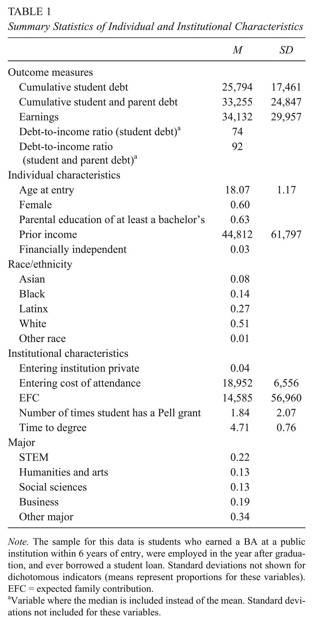
Note. The sample for this data is students who earned a BA at a public institution within 6 years of entry, were employed in the year after graduation, and ever borrowed a student loan. Standard deviations not shown for dichotomous indicators (means represent proportions for these variables). EFC = expected family contribution.

Variable where the median is included instead of the mean. Standard deviations not included for these variables.

A majority of the students in the analytical sample identify as women (60%) and report at least one parent earning at least a bachelor’s degree (63%). The students primarily identify as White (51% of the sample), followed by Latinx (27%), Black (14%), Asian (8%), and other race (1%). The students have an average starting age of 18, a prior income of $44,812 (parents’ income for financially dependent and students’ income for financially independent), and only 3% are classified as financially independent.

On average, these students start college with a cost of attendance around $18,952, which grows by $2,508 by the time the students graduate. Only 4% of the sample started at a private institution (all students graduate from a public Texas institution). The average student who graduates in no more than 6 years takes approximately 5 years to complete their bachelor’s degree. Most students graduate with a bachelor’s degree in a STEM field (22%), followed by business (19%), the humanities and arts (13%), and the social sciences (12%). The rest of the students received degrees in other majors, a category including architecture, communications, personal skills, military sciences, library sciences, and more (aligns with extant literature and National Center for Education Statistics definitions).

A significant number of the students have ever received an EFC of zero, indicating that the family would be unable to contribute to the costs of education for the student (34%). In addition, a little over half (53%) of students ever receive a Pell grant, though, on average, students only received a Pell grant twice during their undergraduate career. The sample of students used in the current work relies more on need-based financial aid than the overall averages for Texas (i.e., in 2015, approximately 40% of undergraduate students received a Pell grant). This is due to the requirement of a financial aid file for students to be included in the analytical sample.

The summary statistics describe a sample that is primarily White, female, and from families with previous experience with higher education. To better understand the student-level characteristics for this sample associated with high debt-to-income ratios, I first discuss the results for Research Question 1.

Characteristics Associated With Total Undergraduate Borrowing (RQ 1)

Exploring the relationship between student-level characteristics and the outcomes across the distribution allows for a deeper understanding of the heterogeneity of associations. This is not just an academic concern; better estimation of the results provides information that might have a direct influence on how institutions could fare if ever held accountable for debt-to-income ratio metrics like the one Texas has created.

To show the differences between OLS and QR, I discuss the traditional OLS estimates first (see Table 2, Column 1). The patterns of association mirror national trends (e.g., College Board, 2015). On average, every additional year of age at the start of entry to postsecondary education is associated with an additional $790 in cumulative undergraduate debt. Black and Latinx students, on average, borrow $7,124 and $453 more than their White peers, while Asian students borrow $3,155 less. When controlling for the other student characteristics, women borrow $323 less than men while students who had at least one parent with a bachelor’s degree borrowed $692 less (compared to peers who had no parents with a bachelor’s degree). Students who first enrolled in private institutions before graduating from a public school are predicted to borrow $1,567 more than students who began at a public school. Students from higher income backgrounds borrow larger amounts than their lower income peers.

Table 2

Relationship Between Student-Level Characteristics and Undergraduate Cumulative Debt (Student Only)

	OLS	10th Percentile	25th Percentile	50th Percentile	75th Percentile	90th Percentile
Age at entry	790.277*** (70.284)	170.904*** (42.164)	550.974*** (77.414)	657.016*** (70.973)	1,044.645*** (112.479)	1,885.060*** (256.788)
Race (reference: White)
Black	7,123.661*** (249.285)	1,975.437*** (157.652)	6,252.830*** (307.099)	7,499.971*** (279.553)	10,037.040*** (398.822)	11,690.884*** (734.455)
Latinx	453.748* (200.788)	−293.758* (144.739)	34.610(270.786)	563.959* (228.256)	748.972* (292.093)	1,338.065** (512.714)
Asian	−3,155.681*** (262.733)	−1,230.715*** (233.161)	−3,771.049*** (424.334)	−3,478.915*** (321.941)	−3,333.395*** (366.377)	−3,122.643*** (597.530)
Other	−287.157(956.233)	−816.684(759.107)	−1,341.698(1,397.992)	−279.148(1,098.133)	894.996(1,362.112)	2,883.141(2,536.569)
Female	−323.455* (151.695)	−185.334(114.235)	−597.748** (212.597)	−154.010(173.772)	−29.757(220.135)	−461.362(390.885)
Parental education (college or higher)	−692.282*** (160.689)	120.336(119.700)	−221.911(217.585)	−390.035* (181.863)	−1,100.899*** (237.281)	−1,193.086** (423.633)
Prior income (log)	1,348.994*** (107.653)	972.917*** (95.633)	1,293.651*** (171.058)	1,239.018*** (131.004)	1,241.547*** (160.130)	2,272.552*** (270.192)
Entry institution private	1,567.695** (480.966)	−595.014* (292.492)	−743.444(559.317)	−333.878(477.400)	2,701.634*** (642.342)	6,920.034*** (1,269.333)
COA entry year (log)	4,495.575*** (299.147)	1,923.673*** (259.589)	3,317.090*** (437.119)	3,680.943*** (347.357)	4,247.006*** (429.611)	7,692.234*** (738.926)
Independent	7,660.008*** (610.914)	2,475.799*** (482.636)	5,271.296*** (814.601)	6,083.920*** (688.334)	11,421.161*** (972.839)	18,310.500*** (1,944.931)
N times student had Pell grant	−380.577*** (52.315)	−151.245*** (40.685)	−99.047(73.786)	−246.609*** (60.963)	119.245(79.658)	−895.620*** (140.789)
Major (reference: STEM)
Humanities and arts	977.603*** (252.601)	941.849*** (194.072)	2,072.697*** (361.593)	1,545.802*** (291.877)	1,080.399** (363.548)	229.854(631.477)
Social sciences	1,960.446*** (256.827)	1,287.509*** (193.598)	2,882.107*** (361.609)	2,412.587*** (293.433)	2,070.310*** (365.813)	2,056.732** (643.417)
Business	1,075.060*** (234.105)	764.684*** (182.466)	1,735.591*** (336.830)	1,442.786*** (266.200)	1,251.717*** (326.331)	1,156.884* (576.416)
Other	1,627.557*** (207.217)	848.551*** (161.985)	2,379.808*** (293.401)	2,113.328*** (234.132)	1,769.838*** (291.351)	1,681.429** (514.683)
Time to degree	4,319.677*** (126.792)	1,296.792*** (93.933)	3,355.735*** (171.910)	4,149.725*** (140.169)	5,515.570*** (182.295)	7,021.020*** (331.742)
Constant	−77,348.709*** (5,518.751)	−34,537.413*** (6,123.347)	−62,170.248*** (9,817.233)	−68,625.351*** (8,335.414)	−78,354.595*** (8,131.337)	−13,7566.688*** (9,449.084)
Observations	55,858	55,858	55,858	55,858	55,858	55,858

Note. Column 1 presents the results from OLS regression. Columns 2 through 6 present the results from unconditional quantile regressions at the corresponding percentile. The models include institution and graduation year fixed effects and heteroskedasticity robust standard errors (in parentheses). OLS = ordinary least squares; COA = cost of attendance.

p < .05. **p < .01. ***p < .001.

Independent students, compared to dependent peers, borrow on average $7,660 more, and the number of times students have a Pell grant during their undergraduate career is associated with a decrease in cumulative undergraduate debt (an additional year of Pell is associated with $381 less in cumulative undergraduate debt). All majors are associated with students borrowing more when compared to their peers who major in STEM. Longer time to degree is also associated with larger amounts of cumulative debt. Therefore, holding all else constant, students who: (a) are Black or Latinx (compared to White peers), older, and financially independent; (b) select certain majors; (c) start at a private or more expensive institution; and (d) take longer to complete a degree are predicted to borrow larger amounts for their undergraduate education.

These OLS estimates are useful to a point. As previously mentioned, there are concerns that OLS estimates may mask additional variation in student-level characteristics’ relationship with students’ borrowing behavior. To demonstrate the usefulness of the QR estimates, I return to the example introduced earlier (potential for race to have a different relationship along the distribution).

Figure 1 presents the quantile regression estimates with 95% confidence intervals for the indicator for Latinx students in the data for all quantiles (100 estimates from 1st to 100th percentile). The OLS estimate for this relationship is included as a dashed horizontal line. The figure makes clear that while the OLS estimate is approximately a positive $400, the positive predicted relationship between being a Latinx student and cumulative undergraduate debt does not truly differentiate from zero until roughly the 50th percentile. In fact, at the lower end of the cumulative debt distribution (e.g., for light borrowers), the predicted relationship between being a Latinx student and cumulative debt is negative (and statistically significantly different from 0).

Figure 1.

Quantile regression estimates of the relationship between cumulative undergraduate debt and Latinx students.

Columns 2 through 6 of Table 2 provide support for this visual assessment. The columns include estimates at the 10th, 25th, 50th, 75th, and 90th percentiles of cumulative undergraduate debt, respectively. At the 10th percentile of cumulative debt, being a Latinx student is associated with $294 less in student loans (compared to a White student), which changes to a $1,338 predicted increase at the 90th percentile. Thus, the majority of the OLS estimate is being driven by the upper end of the distribution. If a state is interested in focusing a policy that targets students at the lower end of the cumulative debt distribution (students with small amounts of undergraduate student loan debt), these results indicate that Latinx students are predicted to borrow less than their White peers (and may not need to be the target of specific policies or programs). In the reverse, if a state is interested in the factors that predict borrowing more at the upper end of the cumulative debt distribution (students with larger amounts of student loan debt), these results indicate that being a Latinx student, compared to a White student, predicts an increase in the accumulation of debt (and may need to be the target of special policies or programs).¹³

Returning to the estimates presented in Table 2, the QR estimates are generally similar to the OLS estimates for age, being Black or Asian, one’s prior income, entry COA, being financially independent, and all majors except the arts. All of these student-level characteristics, except for being Asian, are positively associated with cumulative undergraduate debt in all quantiles. However, there is some variation in estimates for other student characteristics. At the upper end of the cumulative debt distribution (e.g., heavy borrowers), the following student characteristics are predictors of student debt: age at entry; being Black, Latinx, or Asian; parental education; prior income; entering higher education at a private institution; COA during the entry year; being classified financially independent; the number of times a student received the Pell grant; majoring in anything that is not a STEM field; and a longer time to degree.

At the other end of the distribution, predictors of cumulative debt amount also include being a woman and do not include parental education. Therefore, the OLS estimate for women and parental education are being driven by the bottom and upper ends of the cumulative debt distribution, respectively. In addition, while being Latinx and entering higher education at a private institution are predictors at both ends of the distribution, the direction of the relationship changes depending on the quantile. As previously mentioned, being Latinx is negatively associated with cumulative debt at the lower end of the distribution and positively associated at the upper end. The evidence is the same for starting at a private institution.

These findings provide evidence that there is variation in the relationship between cumulative undergraduate debt and being Latinx and a woman, parental education, and the institutional control of first institution enrolled. Next, I review the findings for debt-to-income ratio.

Characteristics Associated With Debt-to-Income Ratio (RQ 2)

The OLS results for debt-to-income ratio are presented in Table 3, Column 1. An additional year of age at entry to college, on average, is associated with a 5-percentage point (pp) larger debt-to-income ratio. On average, Black students have a 47-pp larger debt-to-income ratio than their White peers. Women have a 13-pp larger debt-to-income ratio than men. Students from families with at least one parent who earned a bachelor’s degree have a predicted debt-to-income ratio 10 pp larger than students without a college-educated parent. Students who enroll at a private institution first and then earn a degree from a public institution have a predicted 21-pp larger debt-to-income ratio. Independent students and those who take longer to complete the degree also have higher debt-to-income ratios. Finally, students who major in the social sciences, humanities and arts, and other major category have higher debt-to-income ratios than their peers who major in STEM fields.

Table 3

Relationship Between Student-Level Characteristics and Debt-to-Income Ratio (Student Only)

	OLS	10th Percentile	25th Percentile	50th Percentile	75th Percentile	90th Percentile
Age at entry	4.966** (1.588)	0.532** (0.194)	1.658*** (0.237)	2.473*** (0.432)	3.689*** (1.034)	6.884* (2.753)
Race (reference: White)
Black	46.812*** (5.689)	8.872*** (0.663)	19.572*** (0.890)	37.659*** (1.441)	64.836*** (3.347)	107.128*** (8.923)
Latinx	−0.306(4.076)	−0.025(0.626)	2.174** (0.815)	6.608*** (1.190)	12.275*** (2.511)	22.309*** (6.452)
Asian	0.751(5.687)	−4.885*** (1.140)	−7.031*** (1.390)	−2.222(1.814)	9.385** (3.638)	40.102*** (9.553)
Other	−4.588(15.363)	−2.816(3.435)	−3.959(4.346)	3.444(5.959)	0.238(12.047)	17.758(31.248)
Female	12.696*** (3.281)	3.158*** (0.507)	6.516*** (0.648)	9.779*** (0.924)	10.737*** (1.963)	20.358*** (5.061)
Parental education (college or higher)	10.188** (3.310)	0.347(0.501)	0.405(0.649)	0.318(0.946)	6.164** (2.018)	20.849*** (5.134)
Prior income (log)	4.100(3.151)	1.892*** (0.410)	3.121*** (0.511)	3.715*** (0.698)	7.482*** (1.435)	14.332*** (3.708)
Entry institution private	21.214* (9.699)	−1.551(1.282)	0.932(1.640)	7.121** (2.404)	19.315*** (5.391)	48.019** (14.647)
COA entry year (log)	9.472(4.882)	4.416*** (1.109)	4.443** (1.354)	9.874*** (1.861)	12.132** (3.895)	22.973* (9.787)
Independent	29.648* (11.710)	5.903** (1.984)	6.590** (2.518)	11.752** (3.666)	33.303*** (8.212)	58.818** (21.571)
N times student had Pell grant	−0.696(1.119)	−0.124(0.172)	−0.119(0.220)	0.108(0.318)	0.076(0.682)	0.064(1.765)
Major (reference: STEM)
Humanities and arts	50.072*** (5.214)	10.088*** (0.860)	18.993*** (1.100)	29.212*** (1.590)	50.174*** (3.455)	94.239*** (9.182)
Social sciences	49.549*** (5.728)	13.293*** (0.813)	23.367*** (1.076)	36.705*** (1.579)	56.211*** (3.519)	82.647*** (9.273)
Business	−7.839(4.373)	1.429(0.881)	2.939** (1.069)	−0.218(1.385)	−14.496*** (2.682)	−37.739*** (6.536)
Other	24.945*** (3.986)	6.608*** (0.734)	12.303*** (0.918)	14.164*** (1.264)	20.384*** (2.625)	31.326*** (6.724)
Time to degree	8.695** (3.029)	2.060*** (0.412)	5.080*** (0.519)	7.127*** (0.740)	10.061*** (1.590)	9.322* (4.123)
Constant	−237.439*** (68.202)	−99.214*** (29.787)	−130.193*** (30.039)	−157.806*** (38.323)	−158.828(93.483)	−527.180*** (130.547)
Observations	40,769	40,769	40,769	40,769	40,769	40,769

Note: The outcome debt-to-income ratio is measured as a percentage. Column 1 presents the results from OLS regression. Columns 2 through 6 present the results from unconditional quantile regressions at the corresponding percentile. The models include institution and graduation year fixed effects and heteroskedasticity robust standard errors (in parentheses). OLS = ordinary least squares; COA = cost of attendance.

p < .05. **p < .01. ***p < .001.

I present the estimates of the QR with debt-to-income ratio as the outcome in Table 3, Columns 2 through 6. In general, consistent positive predictors of debt-to-income ratio include: age at entry, being Black, being a woman, prior income, entry year COA, being independent, majoring in any field that is not business, and time to degree. Similar to the quantile regression estimates for cumulative debt, the OLS estimates do mask variation in the relationship between some of the student-level characteristics and debt-to-income ratio. Beyond those previously mentioned characteristics, predictors at the upper end of the debt-to-income distribution (considered to have relatively large debt burdens) include: being Latinx, being Asian, parental education, enrolling at a private institution, and majoring in business. However, parental education and entering higher education at a private institution are not predictors of debt-to-income ratio at the lower end of the distribution (therefore, the OLS estimates for these characteristics are driven by the upper end of the distribution).

In addition, being Latinx or Asian and majoring in business have different relationships with debt-to-income ratio depending on the quantile. At the lower end of the distribution, being Latinx or Asian, compared to being White, predicts a smaller debt-to-income ratio (not statistically significant for Latinx students at conventional levels). However, at the upper end of the distribution (and from the 25th percentile for Latinx students), students are predicted to have debt-to-income ratios larger than their White peers (even though the OLS estimates provide no evidence of a relationship between being Latinx or Asian and larger debt-to-income ratios). For majoring in business, at the lower end of the debt-to-income distribution, the students are predicted to have a smaller debt-to-income ratio than STEM majors. This relationship reverses at the upper end of the distribution.

Therefore, when investigating debt-to-income ratios, I find that being Latinx or Asian, parental education, first enrolling in a private institution, and majoring in business vary in their relationship with debt-to-income ratios.

Sensitivity Analysis

To gauge the practical significance of these results, it is necessary to investigate the sensitivity of the variations in the relationship between student-level characteristics and debt-to-income ratios. First, I estimate the debt-to-income ratio quantile regressions separately for students who have ever had an EFC of zero and students who have never had an EFC of zero (Tables A1 and A2, respectively). I focus on students who have ever or never had an EFC of zero to investigate how the relationship shifts for students based on students’ ability to finance their education. While the majority of the estimates were similar to Table 3, there were some differences. The estimated relationships for students who had ever had an EFC of zero appear to drive the overall results discussed in the prior section for parental education, prior income, and time to degree. Students who had ever had an EFC of zero are consistently predicted to have a higher debt-to-income ratio when their parents have earned a bachelor’s degree. For students who have never had an EFC of zero, this relationship was generally negative (though primarily in the lower distribution of debt-to-income ratios). Also, students with an EFC of zero drive the prior income (which makes sense as the marginal dollar will likely matter more for student financial need estimates of these students and debt accumulation) and time-to-degree results previously reported.

Second, I investigate gender differences, in part, due to persistent research highlighting gender labor market differences (Tables A3 for women and A4 for men). The consistent age results discussed in the prior section are overwhelmingly driven by the female students in the sample. For the relationship between being Asian and debt-to-income ratio, women in the lower portion of the distribution of debt-to-income ratios are consistently predicted to have a lower debt-to-income ratio compared to White women. In contrast, Asian men in the upper portion are consistently predicted to have a higher debt-to-income ratio compared to White men. Turning to major, women who major in business have a consistent, negative predicted association with debt-to-income ratio (compared to majoring in STEM). However, men who major in business are predicted to have a higher debt-to-income ratio (particularly in the lower end of the distribution).

Third, I investigate how the estimates shift if I include students who did not earn a credential (Table A5).¹⁴ The relationships are qualitatively similar to Table 3 (which was estimated only for students who earned a bachelor’s degree). The primary difference is that the age estimates are no longer statistically significant and parental education is now consistently positive and statistically significant across the distribution of debt-to-income ratio. Also, being Latinx is now a negative predictor of debt-to-income ratio at the lower end of the distribution (compared to White students).

Discussion

I find evidence that while some student-level characteristics are consistently associated with cumulative debt or debt-to-income ratios, there are a number of characteristics that differ. I find variation in cumulative debt’s relationship with Latinx students, women, parental education, and institutional control of first institution enrolled. I also find evidence of variation in debt-to-income ratio’s relationship with Latinx students, Asian students, parental education, institutional control of first institution enrolled, and majoring in business. In several cases, the predicted relationship between these student-level characteristics is different than standard analyses (OLS regression) would suggest. This variation suggests that solely focusing on the relationship between the “average” student and debt-to-income ratios may not be enough to control the debt burden of bachelor’s degree earners.

Standard analysis would predict that the student characteristics associated with a higher debt-to-income ratio (and therefore more likely to increase the state’s debt-to-income ratio) are older students, Black students, women, and students with at least one parent with a bachelor’s degree. This type of analysis would also indicate that students who first enrolled at a private institution, are classified as financially independent, take longer to graduate, or major in non-STEM and non-business fields are associated with larger debt-to-income ratios. However, when I inspect the distribution of debt-to-income ratios, I also find that Latinx and Asian students at the upper end of the debt-to-income ratio distribution (larger debt burdens) are predicted to have a larger debt-to-income ratio than White students. I also find evidence that a higher COA in the first year predicts a larger debt-to-income ratio at higher percentiles of debt-to-income ratio. Relying solely on standard analysis might mask the ways that these other student-level characteristics are associated with debt burden (operationalized as debt-to-income ratio).

With these variations in mind, a higher education strategic maintenance goal or policy like the DBCG generally would require a focus on the student-level characteristics associated with the upper end of the debt-to-income distribution (since the threshold is 60%). Institutional sanctions attached to this type of threshold could have unintended consequences. Based on the quantile regressions, institutions that serve a significant number of students with the characteristics most associated with the upper end of the debt-to-income distribution likely would be disproportionately affected by an accountability tool like the Texas DBCG (if calculated at the institution level).

I investigated which Texas public institutions are above the debt-to-income threshold of 60%. When I do this, I find that 18 institutions have a median debt-to-income of at least 60% (including only student debt). In the institutions with the top 5 median debt-to-income ratios, 2 are the only public four-year Historically Black Colleges or Universities in Texas (Prairie View A&M University and Texas Southern University), and the others are regional institutions across the state of Texas (Stephen F. Austin State University, Texas A&M University-Commerce, and University of North Texas at Dallas). These regional institutions also happen to have significant numbers of Black and Latinx students enrolled. Even when using both student and parent loans in the measure of undergraduate debt, the list is virtually unchanged (the University of North Texas replaces Texas A&M University-Commerce, though Commerce is still in the top 10 institutions). This would imply that certain types of institutions, by educating different student populations, would have a larger median debt-to-income ratio. Scholars have cautioned that accountability measures for higher education institutions must take into consideration the demographic composition of students because this can and likely does influence the outcomes of interest to the state or federal government (Flores, Park, & Baker, 2017, 2018). This same caution should be applied when evaluating institutions on the debt-to-income ratios of their students.

Further, returning to the education triage example from NCLB, if the focus at institutions and the state became the 60% threshold, then less attention could be paid to students with at least one parent with a bachelor’s degree or Asian students, who are only predicted to have a higher debt-to-income ratio starting around the 75th percentile of debt-to-income ratio (which is supported by the Appendix Figures A2h and A2d). This is true whether I measure debt-to-income ratios with just student debt or student and parent debt.¹⁵ Also, students who started at private institutions and transitioned to public institutions, who would be counted in a debt burden metric like the one in Texas, have a stronger relationship with debt-to-income ratios at the upper end of the distribution. This could create an unintended policy consequence of institutions making selective transfer admission decisions based on the potential effect to their debt-to-income ratio.

Overall, states other than Texas potentially could use debt-to-income ratios as an accountability tool for either the entire state or individual higher education institutions (e.g., via inclusion in a performance-based funding model). This work highlights some of the possible challenges to using this type of measure for accountability. This is not an exhaustive list. For example, women are predicted to have higher debt-to-income ratios and smaller cumulative debt amounts (though there is variation in the subpopulation estimates focused only on women). This is due, in part, to differences in the income of women.¹⁶ It is difficult to know what institutions are supposed to do about labor market discrimination against women.

If a state were interested in adopting a similar measure, it would be important to either construct a statewide threshold without sanctions or, if focused on individual institutions, adjust for the demographics of those institutions. For example, scholars have found evidence that performance-based funding can differentially affect institutions that enroll large numbers of racial/ethnic minority students (e.g., Jones, 2014; Umbricht, Fernandez, & Ortagus, 2017). Due to this, several states have added premiums that adjust the calculation of how well an institution is performing based on the number of underserved students enrolled (Gandara & Rutherford, 2017; Kelchen, 2018a). Researchers have found that these premiums have mixed results, helping some underserved student groups enroll more and hurting others (e.g., Gandara & Rutherford, 2017), but the need for adjustment is clear.

The state of Texas has emphasized that debt-to-income ratios of certain institutions or sectors will not be held to the 60% threshold (THECB, 2016). Even without sanctions, it is not clear how feasible the DBCG is. For example, how will the state balance the structural barriers to financing higher education and within the labor market with its strategic goals in light of the demographic changes over the coming decades, which include a continued increase in the number of Latinx and Black students in the Texas higher education system (Fernandez et al, 2016)? It is not clear how other states should balance the same demographic realities with desires for increased accountability on college affordability.

Conclusion

Texas is the first state to create a strategic goal for the debt-to-income ratio of its graduates. This is an admirable goal and demonstrates the state’s commitment to ensuring that attaining a college degree is affordable and graduates can attain jobs with salaries that would allow them to repay their debt in a reasonable manner. Still, more research is needed to evaluate the potential effect of either publishing institutional debt-to-income ratios (as a low-stakes accountability measure) or assigning penalties to institutions with debt-to-income ratios above the threshold. This last point is particularly critical for other states that are investigating the potential to create their own version of this goal. Demographic composition of institutions could unduly influence their median debt-to-income ratios.

Texas’s DBCG does not take into consideration the repayment plan that students select for their student loans. This choice is due to the reality that the state does not have access to data on the repayment behaviors of any of their students on federal student loans. There is little research on when the ratio of total undergraduate debt to income becomes indicative of financial hardship. This is likely due, in part, to the variability in students’ repayment plan selection, which can potentially ameliorate some of the concerns of higher total debt-to-income ratios when compared with actual repayment amount–to–income ratios. Additional research needs to be conducted to investigate the relationship between these two different measures of debt burden to find the scenarios or contexts that are appropriate for the use of the total debt-to-income ratio. Texas, and other states in general, does not have access to another measure of debt burden and therefore will be unlikely to use another. It is therefore essential that policymakers are provided with a better understanding of when and how this measure can be used appropriately.

Furthermore, it would be useful to investigate how volatile the earnings estimates are when both graduates and students who do not earn credentials are included in the debt-to-income ratio. As highlighted in the sensitivity analysis, when I estimated the relationship between student-level characteristics and debt-to-income ratios including nongraduates, I found qualitatively similar estimates to the ones presented in the current work (particularly in the upper end of the debt-to-income distribution). This gives some support to the THECB only using students who earned a credential in the ratio, though it also would be useful to analyze the robustness of these estimates for students earning other types of credentials and for including a ratio that includes more than a single year of earnings. It could be that there is something different about students who begin higher education at a 4-year institution. It also could be that the salaries of bachelor’s degree earners are compressed in the first year after earning a credential due the composition of students who immediately enter the workforce after graduating.

This work highlights many areas that evidence suggests could be the focus of state policymakers to create better targeted policies to decrease the amount of debt burden facing students. While not causal, the current research provides support for the importance of long-term policy planning based on current and projected demographics. The types of goals like the ones found in 60x30TX demonstrate the real interest and concern policymakers have for college graduates with significant debt burdens. The difficulty ahead lies in determining the best incentives or interventions to create the structures necessary to help students navigate their life after college successfully.

Footnotes

Appendix

Table A5

Relationship Between Student-Level Characteristics and Debt-to-Income Ratio for Graduates and Nongraduates

	OLS	10th Percentile	25th Percentile	50th Percentile	75th Percentile	90th Percentile
Age at entry	2.663* (1.277)	−0.091 (0.139)	0.074 (0.177)	0.308 (0.267)	0.587 (0.590)	2.252 (1.595)
Race (reference: White)
Black	26.935*** (4.065)	6.476*** (0.492)	13.595*** (0.715)	27.253*** (1.176)	45.555*** (2.664)	74.217*** (7.034)
Latinx	−10.275** (3.446)	−1.410** (0.477)	−1.421* (0.660)	1.092 (1.015)	0.919 (2.123)	−0.200 (5.386)
Asian	7.299 (9.420)	−2.642** (0.822)	−5.918*** (1.151)	−8.068*** (1.686)	−3.357 (3.433)	15.088 (9.023)
Other	10.097 (15.441)	1.276 (2.313)	−0.138 (3.320)	0.570 (5.044)	2.723 (10.207)	23.357 (26.952)
Female	16.081*** (2.796)	5.265*** (0.360)	8.641*** (0.494)	13.455*** (0.745)	16.859*** (1.561)	18.865*** (3.997)
Parental education (college or higher)	17.286*** (2.922)	2.601*** (0.369)	4.429*** (0.508)	7.223*** (0.783)	15.757*** (1.669)	34.737*** (4.280)
Prior income (log)	21.840*** (2.296)	4.471*** (0.284)	8.384*** (0.383)	13.370*** (0.563)	24.004*** (1.150)	46.629*** (2.959)
Entry institution private	31.533 (20.184)	−4.430* (1.936)	−0.782 (2.270)	4.511 (3.461)	11.392 (8.249)	11.392 (19.983)
COA entry year (log)	30.591*** (5.197)	9.063*** (0.829)	13.916*** (1.092)	18.406*** (1.559)	27.057*** (3.198)	47.019*** (7.903)
Independent	28.079*** (7.854)	5.471*** (1.300)	9.149*** (1.730)	13.082*** (2.573)	34.422*** (5.531)	70.369*** (14.745)
N times student had Pell grant	13.866*** (0.903)	2.177*** (0.112)	4.466*** (0.153)	7.838*** (0.236)	14.321*** (0.524)	27.957*** (1.431)
Constant	−519.421*** (54.840)	−130.135*** (9.359)	−218.135*** (12.115)	−294.156*** (17.226)	−467.350*** (35.427)	−869.913*** (88.977)
Observations	57,430	57,430	57,430	57,430	57,430	57,430

Note: Column 1 presents the results from OLS regression. Columns 2 through 6 present the results from unconditional quantile regressions at the corresponding percentile. The models include institution and graduation year fixed effects and heteroskedasticity robust standard errors (in parentheses). OLS = ordinary least squares; COA = cost of attendance.

p < .05. **p < .01. ***p < .001.

Acknowledgements

The author would like to thank Christopher Bennett, Benjamin Skinner, Denisa Gándara, Sondra Barringer, Richard Blissett, and Stephen DesJardins for their helpful comments. The author bears sole responsibility for the content of this article. This study was supported by a grant through the Texas OnCourse Research Network. The data used in this study come from the Texas Education Research Center. The conclusions of this research do not necessarily reflect the opinion or official position of Texas OnCourse, the Texas Education Research Center, the Texas Education Agency, the Texas Higher Education Coordinating Board, the Texas Workforce Commission, or the State of Texas.

ORCID iD

Dominique J. Baker

Notes

Author

DOMINIQUE J. BAKER is an assistant professor of education policy in the Annette Caldwell Simmons School of Education and Human Development and an associate in the John Goodwin Tower Center for Political Studies. Her research focuses on the way that education policy affects and shapes the access and success of underrepresented students in higher education.

References

American Association of University Women. (2017). Deeper in debt: Women and student loans. Washington, DC: Author.

Avery

Turner

(2012). Student loans: Do college students borrow too much—or not enough? Journal of Economic Perspectives, 26(1), 165–192.

Baker

D. J.

Doyle

W. R.

(2017). Impact of community college student debt levels on credit accumulation. The ANNALS of the American Academy of Political and Social Science, 671(1), 132–153.

Ballou

Springer

M. G.

(2017). Has NCLB encouraged educational triage? Accountability and the distribution of achievement gains. Education Finance & Policy, 12(1), 77–106.

Baum

O’Malley

(2003). College on credit: How borrowers perceive their education debt. Journal of Student Financial Aid, 33(3), 7–19.

Baum

Schwartz

(2006). How much debt is too much? Defining benchmarks for manageable student debt. Washington, DC: The Project on Student Debt and The College Board.

Belfield

(2013). Student loans and repayment rates: The role of for-profit colleges. Research in Higher Education, 54(1), 1–29.

Chapman

Dearden

(2017). Conceptual and empirical issues for alternative student loan designs: The significance of loan repayment burdens for the United States. The ANNALS of the American Academy of Political and Social Science, 671(1), 249–268.

College Board. (2014). Trends in student aid 2014. Washington, DC: Author.

10.

College Board. (2015). Trends in student aid 2015. Washington, DC: Author.

11.

Perlmeter

E. R.

(2014). Texas consumer credit series: Student loans part 1: Get the numbers right. Retrieved from http://www.dallasfed.org/microsites/cd/perspectives/articles/2014/1202.html

12.

Fernandez

Fletcher

Klepfer

(2016). State of student aid and higher education in Texas. Retrieved from https://www.tgslc.org/pdf/SOSA.pdf

13.

Firpo

Fortin

N. M.

Lemieux

(2009). Unconditional quantile regression. Econometrica, 77(3), 953–973.

14.

Flores

S. M.

Park

T. J.

Baker

D. J.

(2017). The racial college completion gap: Evidence from Texas. Journal of Higher Education, 88(6), 894–921.

15.

Flores

S.M.

Park

T. J.

Baker

D. J.

(2018). Accountability across the educational pipeline: The contribution of unequal high schools on college completion. In Orfield

Hillman

(Eds.), College opportunity and accountability: The civil rights dimension (pp. 89–110). Cambridge, MA: Harvard Education Press.

16.

Florida

(2016, March 15). The U.S. cities winning the battle against brain drain. Retrieved from https://www.citylab.com/life/2016/03/which-metros-are-best-at-keeping-their-college-graduates/473604/

17.

Gándara

Rutherford

(2018). Mitigating unintended impacts? The effects of premiums for underserved populations in performance-funding policies for higher education. Research in Higher Education, 59(6), 681–703.

18.

Gillborn

Youdell

(2000). Rationing education: Policy, practice, reform and equity. Philadelphia, PA: Open University Press.

19.

Gross

Cekic

Hossler

Hillman

(2009). What matters in student loan default: A review of the research literature. Journal of Student Financial Aid, 39, 19–29.

20.

Hillman

N. W.

(2014). College on credit: A multilevel analysis of student loan default. Review of Higher Education, 37(2), 169–195.

21.

Hillman

(2015). Borrowing and repaying student loans. Journal of Student Financial Aid, 45(3), 35–48.

22.

Houle

J. N.

(2013). Disparities in debt: Parents’ socioeconomic resources and young adult student loan debt. Sociology of Education, 87(1), 53–69.

23.

Jones

(2014). Performance funding at MSIs: Considerations and possible measures for public minority-serving institutions. Atlanta, GA: Southern Education Foundation.

24.

Kelchen

(2017). Tuition control policies: A challenging approach to college affordability. Midwestern Higher Education Compact Policy Brief. Retrieved from https://www.mhec.org/sites/default/files/resources/mhec_affordability_series3_20170824.pdf

25.

Kelchen

(2018a). Do performance-based funding policies affect underrepresented student enrollment? Journal of Higher Education, 89(5), 702–727.

26.

Kelchen

(2018b). Higher Education Accountability. Baltimore, MD: Johns Hopkins University Press.

27.

Kelchen

Pingel

(2018). Postsecondary tuition capping and freezing. Retrieved from https://www.ecs.org/postsecondary-tuition-capping-and-freezing/

28.

Kim

M. M.

(2015). The impacts of state control policies on college tuition increase. Educational Policy, 29(5), 815–838.

29.

Looney

Yannelis

(2015). A crisis in student loans? How changes in the characteristics of borrowers and in the institutions they attended contributed to rising loan defaults. Retrieved from http://www.brookings.edu/~/media/projects/bpea/fall-2015/looneytextfallbpea.pdf

30.

MacLean

J. C.

Webber

D. A.

Marti

(2014). An application of unconditional quantile regression on cigarette taxes. Journal of Policy Analysis and Management, 33(1), 188–210.

31.

Malcom

L. E.

Dowd

A. C.

(2012). The impact of undergraduate debt on the graduate school enrollment of STEM baccalaureates. Review of Higher Education, 35(2), 265–305.

32.

Martins

P. S.

Pereira

P. T.

(2004). Does education reduce wage inequality? Quantile regression evidence from 16 countries. Labour Economics, 11, 355–371.

33.

McKinney

Hagedorn

L. S.

(2017). Performance-based funding for community colleges: Are colleges disadvantage by serving the most disadvantaged students? Journal of Higher Education, 88(2), 159–182.

34.

National Conference of State Legislatures. (2015). Performance-based funding for higher education. Retrieved from http://www.ncsl.org/research/education/performance-funding.aspx

35.

Neal

Schanzenbach

D. W.

(2010). Left behind by design: Proficiency counts and test-based accountability. Review of Economics and Statistics, 92(2), 262–283.

36.

Office of Postsecondary Education, U.S. Department of Education. (2014). Program integrity: Gainful employment. Federal Register, 79(211), 64890–65103.

37.

Porter

S. R.

(2014). Quantile regression: Analyzing changes in distributions instead of means. In Paulsen

M. B.

(Ed.), Higher education: Handbook of theory and research (pp. 335–381). New York, NY: Spring Publishing Company.

38.

Price

D. V.

(2004). Educational debt burden among student borrowers: An analysis of the Baccalaureate & Beyond panel, 1997 follow-up. Research in Higher Education, 45(7), 701–737.

39.

Rothstein

Rouse

C. E.

(2011). Constrained after college: Student loans and early-career occupational choices. Journal of Public Economics, 95, 149–163.

40.

Rothwell

(2015). What colleges do for local economies: A direct measure based on consumption. Retrieved from https://www.brookings.edu/research/what-colleges-do-for-local-economies-a-direct-measure-based-on-consumption/

41.

Tandberg

Laderman

Carlson

(2017). A federal-state partnership for true college affordability. Boulder, CO: State Higher Education Executive Officers Association.

42.

Texas Higher Education Coordinating Board. (2015). Texas higher education strategic plan: 2015–2030. Retrieved from http://www.thecb.state.tx.us/reports/PDF/9306.PDF?CFID=65439313&CFTOKEN=76929509

43.

Texas Higher Education Coordinating Board. (2016). Texas public higher education almanac: A profile of state and institutional performance and characteristics. Retrieved from http://www.thecb.state.tx.us/reports/DocFetch.cfm?DocID=7831&Format=PDF

44.

Texas Higher Education Coordinating Board. (2017). Student debt. Retrieved from http://www.txhigheredaccountability.org/acctpublic/#goal4

45.

Umbricht

M. R.

Fernandez

Ortagus

J. C.

(2017). An examination of the (un)intended consequences of performance funding in higher education. Educational Policy, 31(5), 643–673.

46.

University of Wisconsin System. (2017). Regents approve outcomes-based metrics, faculty workload policies. Retrieved from https://www.wisconsin.edu/news/archive/regents-approve-outcomes-based-metrics-faculty-workload-policies/

47.

Urban Institute. (2017). Understanding college affordability. Retrieved from http://collegeaffordability.urban.org/covering-expenses/state-policies/#/.

48.

Webber

D. A.

Ehrenberg

R. G.

(2010). Do expenditures other than instructional expenditures affect graduation and persistence rates in American higher education? Economics of Education Review, 29, 947–958.

49.

Woo

Bentz

Lew

Smith

Velez

E. D.

(2017). Repayment of student loans as of 2015 among 1995–96 and 2003–04 first-time beginning students: First look (NCES 2018-410). Washington, DC: National Center for Education Statistics.

When Average Is Not Enough: A Case Study Examining the Variation in the Influences on Undergraduate Debt Burden

Abstract

Keywords

Literature Review

Student Loan Repayment

Texas Policy Context

Method

Data

Analytic Method

Limitations

Results

Summary Statistics

Characteristics Associated With Total Undergraduate Borrowing (RQ 1)

Characteristics Associated With Debt-to-Income Ratio (RQ 2)

Sensitivity Analysis

Discussion

Conclusion

Footnotes

Appendix

Acknowledgements

ORCID iD

Notes

Author

References