Sage Journals: Discover world-class research

Abstract

Cochlear implant (CI) users, even with substantial speech comprehension, generally have poor sensitivity to pitch information (or fundamental frequency, F0). This insensitivity is often attributed to limited spectral and temporal resolution in the CI signals. However, the pitch sensitivity markedly varies among individuals, and some users exhibit fairly good sensitivity. This indicates that the CI signal contains sufficient information about F0, and users’ sensitivity is predominantly limited by other physiological conditions such as neuroplasticity or neural health. We estimated the upper limit of F0 information that a CI signal can convey by decoding F0 from simulated CI signals (multi-channel pulsatile signals) with a deep neural network model (referred to as the CI model). We varied the number of electrode channels and the pulse rate, which should respectively affect spectral and temporal resolutions of stimulus representations. The F0-estimation performance generally improved with increasing number of channels and pulse rate. For the sounds presented under quiet conditions, the model performance was at best comparable to that of a control waveform model, which received raw-waveform inputs. Under conditions in which background noise was imposed, the performance of the CI model generally degraded by a greater degree than that of the waveform model. The pulse rate had a particularly large effect on predicted performance. These observations indicate that the CI signal contains some information for predicting F0, which is particularly sufficient for targets under quiet conditions. The temporal resolution (represented as pulse rate) plays a critical role in pitch representation under noisy conditions.

Keywords

cochlear implant pitch computational modeling deep learning

Introduction

Cochlear implants (CIs) have been promising choices to restore or improve the hearing ability of people with severe to profound hearing loss. A typical CI device extracts amplitude envelopes of multiple sub-bands and delivers electrical pulses amplitude modulated with the envelopes through a multi-channel electrode placed along the cochlear duct to directly stimulate auditory nerves (Loizou, 1999). A scoping review by Boisvert et al. (2020), for example, reported that the implantation resulted in an improved mean score for monosyllabic words and sentence perception under a quiet condition. Furthermore, many sophisticated CI devices and speech-processing strategies have been proposed to improve speech perception (Carlyon & Goehring, 2021; Clark, 2015; Peterson et al., 2010; Wilson & Dorman, 2008; Zeng et al., 2008). Nevertheless, even modern CI devices cannot compensate for aspects of hearing functions that are important in daily life, such as speech perception under noisy conditions (Boisvert et al., 2020; Friesen et al., 2001), music appraisal (Drennan & Rubinstein, 2008; Limb & Roy, 2014; McDermott, 2004), and sound localization (Dorman et al., 2016; Verschuur et al., 2005).

The present study is concerned with the difficulty of pitch perception by CI users (Geurts & Wouters, 2001; Gfeller et al., 2002; Nimmons et al., 2008; Sucher & McDermott, 2007; Vandali et al., 2005). Pitch is a fundamental aspect of auditory sensation and plays important roles in a variety of perceptions such as music, paralinguistics, tonal languages (e.g., Mandarin), and auditory grouping and selective listening (McDermott & Oxenham, 2008; Oxenham, 2008, 2012).

CI users generally exhibit difficulty in pitch perception across major speech coding strategies (Vandali et al., 2005) and among stimuli or tasks (Kang et al., 2009; McDermott, 2004; Nimmons et al., 2008; Swanson et al., 2019; Zeng et al., 2014). Sucher and McDermott (2007), for example, reported that the pitch ranking by CI users was significantly worse than those by a normal hearing group, assessed using vowels with a fundamental frequency (F0). This insensitivity to pitch negatively impacts the quality of life of CI users (Prevoteau et al., 2018).

The difficulty in perceiving pitch could be attributed to device-oriented, patient-oriented, and surgical-oriented factors. The device-oriented factor includes the constraints of the acoustic information conveyed by the CI signal (Limb & Roy, 2014). The temporal pitch constraint of the CI signal is introduced by coarse-envelope representation by discrete pulse trains at a fixed pulse rate (in pulses per second, pps). The majority of CI users exhibited challenges in discriminating rate pitch above approximately 300 Hz (Carlyon et al., 2010; Moore & Carlyon, 2005; Vandali et al., 2013; Venter & Hanekom, 2014; Zeng, 2002; Zhou et al., 2019). The place-pitch information is constrained by the number of electrode channels (12–24), which inherently lacks the ability to transmit finely graded spectral information typically conveyed by inner hair cells in a healthy cochlea (around 3,500). Under current technical constraints, the best combination of those temporal and spectral specifications has been sought to maximize the efficiency for speech comprehension, and pitch perception has not been the primary interest. Thus, it is arguable that the current CI configurations are not generally optimal for pitch perception across CI users.

We should note, however, that there is a large variety of pitch sensitivity across CI users (Bissmeyer et al., 2020; Goldsworthy & Shannon, 2014; Kenway et al., 2015; Kong & Carlyon, 2010; Looi et al., 2004; Ping et al., 2012; Townshend et al., 1987) and those with high sensitivity can discriminate as small as a one-semitone difference (Nimmons et al., 2008). This indicates the possibility that the CI signal contains sufficient information necessary for F0 estimation, particularly in quiet conditions, and patient/surgical-oriented factors are the main bottlenecks for pitch perception. To argue the relative contributions of the limiting factors for pitch perception by individuals or populations of CI users, it is important to identify the upper limit of pitch-related information contained in the CI signals with various combinations of the pulse rate and number of channels.

One approach to estimating the information content is to measure the pitch sensitivity of normal-hearing listeners presented with vocoded stimuli simulating CI signals. Earlier studies used this approach to examine how much spectral resolution or number of channels is needed to achieve sufficient pitch perception (Crew & Galvin, 2012; Kong et al., 2004; Mehta & Oxenham, 2017). The results suggested that as many as 16–32 channels would be required for the listener to identify a melody sufficiently. It should be noted that the acoustical signals were synthesized with noise- or sinewave-vocoders. The noise or sinewaves in the signal may interfere with pitch perception, possibly leading to an overestimation of the required spectral resolution for adequate pitch perception. It is important to note also that this approach is applicable only to listeners with normal auditory development, thus cannot capture the contribution of neuroplasticity in the auditory system. When we consider that CI is generally effective for prelingually deaf children with early implantation (Kral & Sharma, 2012; Nagels et al., 2024; Naik et al., 2021; Nicholas & Geers, 2007; Nikolopoulos et al., 1999; Niparko et al., 2010), the upper limit of F0 estimation, with appropriate neural plasticity, may be higher than that estimated for normal-hearing listeners with vocoded-signals.

Another approach for finding the upper limit is to evaluate pitch discrimination by using a computational model. Erfanian Saeedi et al. (2014, 2017) examined the place and temporal features extracted from simulated CI signals and reported that a 4-semitone difference or more in F0 is required to discriminate between two stimuli using the criterion of accuracy. One concern with those studies is that they focused on pre-extracted input features, namely place and temporal cues, which were chosen on the basis of the researchers’ assumptions. Useful but non-obvious cues for pitch estimation may have been overlooked, which may lead to underestimating the actual amount of information contained in the CI signal. We also point out that those previous studies (Erfanian Saeedi et al., 2014, 2017) examined only artificial speech sounds, not naturalistic musical sounds.

We aimed to estimate the upper bound of F0 information more directly from the CI signal. We constructed a computational model that receives (simulated) CI pulse signals as inputs (CI model) rather than pre-extracted features. We also examined a computational model with raw waveform input (waveform model), which is an upper-bound model where all information of a sound is available. The models are deep neural networks (DNNs), data-driven estimators of F0 information, modified from a DNN model that can track the F0 of acoustic signals with very high accuracy (Kim et al., 2018). To evaluate the effect of spectral and temporal resolution on F0 estimation, the simulated CI signals were generated by varying the numbers of channels and pulse rates. The CI pulse input was obtained from a monophonic signal consisting of instrumental or singing sounds that would be encountered in daily life. To explore the adverse effect of noise on the accuracy of F0 estimation, we also included stimulus conditions in which inputs to the CI simulator (or the raw waveform for the waveform model) were superimposed on real-recorded stationary noise. The stimulus conditions with and without noise are referred to as noisy and quiet conditions, respectively. We trained the models with a dataset consisting of a mixture of quiet and noisy conditions and evaluated the models separately for the two stimulus conditions. Training and evaluation were conducted using entirely separate samples (i.e., a held-out evaluation set) to prevent data leakage. As the CI models were trained with systematically varying numbers of channels and pulse rates, we analyzed the relative contributions of place-of-excitation and timing-of-stimulation cues in CI stimulation patterns for F0 estimation. To provide a deeper analysis of the interaction between the fidelity of temporal cues and the F0 range to be estimated, we also varied the temporal-envelope cues by adjusting the cut-off frequency of the low-pass filter used for envelope extraction.

For the reader's convenience, the abbreviations used in this paper are summarized in Table 1.

Table 1.

Summary of Abbreviations

Abbreviation	Meaning
CI	Cochlear implant
F0	Fundamental frequency
DNN	Deep neural network
pps	Pulses per second
Waveform model	Raw waveform input model
CI model	CI signal input model
Env model	Intact envelope input model
RAU	Rationalized arcsine units

Materials and Methods

F0-Estimation Model

To estimate the F0 information in the CI signal, we constructed the waveform and CI models on the basis of Convolutional Representation for Pitch Estimation (CREPE) (Kim et al., 2018).¹ The procedures for F0 training and evaluation are summarized in Figure 1. The waveform model is trained using raw waveform signals and produces each probability corresponding to discrete F0 values in cents. Note that a cent is a unit of measurement for musical intervals, with one cent being one-hundredth of a semitone. A semitone corresponds to a frequency difference of approximately 5.95%. During optimization, the model uses binary cross-entropy loss with F0 labels applied with Gaussian smoothing to soften penalties for nearly correct predictions (Bittner et al., 2017). The CI model serves as the counterpart to the waveform model, taking simulated CI pulse signals as input instead of raw waveform signals. In the prediction phase, the model's estimation is a weighted average over a specified range (e.g., ±3 in Figure 1) centered on a node with the highest probability. Further details are provided below, and the details of the DNN model and training configuration are elaborated in Supplemental Material A.

Figure 1.

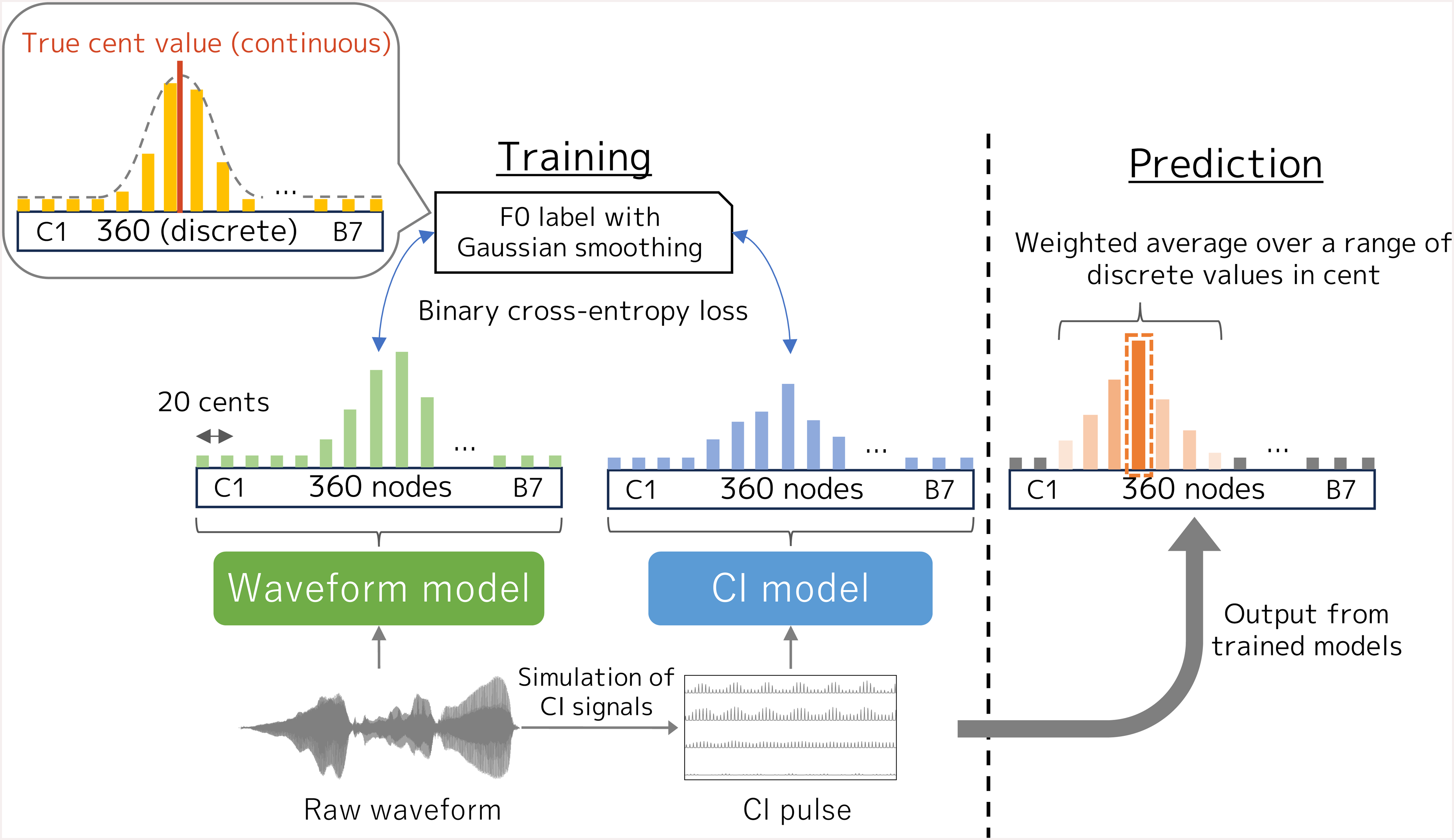
Overview of training and prediction schemes for waveform and CI models. Left and right panels illustrate training and prediction processes, respectively.

The models’ training and estimation target was the discrete values $f_{i}$ ( $i \in {1, \dots, 360}$ ) of F0 ranging from 32.7 Hz (C1) to 3,951.07 Hz (B7) and was divided into 359 intervals of a width of 20 cents (one-fifth of a semitone); hence, the dimensions of the final linear layer used in the models was 360. The value in cents $i$ corresponding to $f_{i}$ was calculated from the following function:

i = 1200 \log_{2} \frac{f_{i}}{f_{r e f}},

where

f_{r e f}

denotes a reference frequency and was 10 Hz for all experiments.

To train the models, the binary cross-entropy loss $L_{B C E}$ was computed from the output probability of each node ${\hat{y}}_{i}$ of the final layer and target label $y_{i}$ as follows:

L_{B C E} = \sum_{i = 1}^{360} (- y_{i} \log {\hat{y}}_{i} - (1 - y_{i}) \log (1 - {\hat{y}}_{i})) .

Since the frequency or cent values are continuous and a ground-truth label

_{gt}

contained in the datasets did not necessarily match with

_{i}

_{gt}

cannot be assigned to a one-hot vector. Therefore,

y_{i}

was determined from a soft label on the basis of Gaussian smoothing

y_{i} = \exp (- \frac{(_{i} -_{gt})^{2}}{2_{std}^{2}}),

where

_{gt}

is in cents, and the standard deviation

_{std}

was fixed to 25 cents in all experiments. As a result, the

y_{i}

was treated as the magnitude of the cent bin covering 20 cents, and the CI and waveform models were dedicated to solving a multi-label classification task and estimating each magnitude. In accordance with CREPE (Kim et al., 2018)¹, when evaluating the chosen model, the estimation results ^∧ were derived from the weighted average over a range of discrete values from

_{j - k}

_{j + k}

, where j is index having the maximum probability of

{\hat{y}}_{i}

\hat{=} \frac{\sum_{i = j - k}^{j + k} {\hat{y}}_{i} i}{\sum_{i = j - k}^{j + k} {\hat{y}}_{i}}, j = \underset{i}{a r g m a x} {\hat{y}}_{i} .

In this experiment, k was set to 4. To estimate the performance variability due to the random initialization of DNN parameters, the models with five variations each were trained by initializing parameters with different random seeds.

Training and Test Datasets

Datasets for Model Training

To train and evaluate the waveform and CI models, we conducted the experiment with three open-access datasets: MDB-stem-synth (Salamon et al., 2017), bach10 (Duan et al., 2010), and nsynth (Engel et al., 2017). The datasets contain singing and instrumental sounds consisting of a single musical note or melody to simulate situations that could be listened to in daily life. The sounds were represented with a sampling frequency of 16 kHz and 16-bit quantization. MDB-stem-synth and nsynth contain only monophonic sounds, and bach10 contains monophonic and polyphonic sounds, but only the monophonic part was used in this study. All datasets contain clear F0 annotations and corresponding time information; hence, the sound portion for training was extracted with 1,024 points centered on that time point. The nsynth dataset (Engel et al., 2017) had been initially partitioned into training, development, and evaluation sets, but MDB-stem-synth (Salamon et al., 2017) and bach10 (Duan et al., 2010) were not. Since each file for those two datasets was composed for each piece of music, the files were divided per piece of music to ensure that similar timbres and F0s were not included in the training and evaluation set (i.e., preventing data leakage). Specifically, the number of files was split into a 3:1:1 ratio for the training:development:test sets in each dataset. Therefore, the amount of combined data after partitioning was 121.8, 22.2, and 80.1 hours for training, development, and test, respectively.

In addition to the above datasets consisting of the target sounds in isolation (quiet condition), we generated noisy-conditioned datasets in which the above data were superimposed with samples from the noise dataset JEIDA-NOISE (Itahashi, 1990). This was done to simulate daily situations in which signals of interest are mixed with background noise. JEIDA-NOISE consists of 17 types of real-recorded sources featuring mostly stationary environmental noise. Specifically, it includes two types of in-car noise, two types of exhibition hall noise, station noise, telephone-booth noise, two types of factory noise, highway noise, crowd noise, two types of train noise, two types of computer-room noise, two types of air-conditioner noise, and elevator lobby noise. The total duration of this noise dataset is 66.7 hours. Since very few recordings in this dataset had a clear F0 or explicit harmonic structures, there was no need to relabel the F0 values in the training data when simulating natural noisy conditions. The noise data in JEIDA-NOISE has power concentrated in a low-frequency band similar to pink noise. During superimposing, 1,024 segments were randomly selected from among all sound sources, and the signal-to-noise ratio (SNR) was randomly selected from 0 to 15 dB. This SNR range is based on common everyday listening situations (Smeds et al., 2015). We evaluated the waveform and CI models trained with mixed data of quiet and noisy conditions.

Datasets for Model Evaluation

The evaluation process was conducted on two realistic test sets simulating sounds that could be encountered in daily life. The evaluation data simulated quiet and noisy conditions as described in Section “Datasets for Model Training”. The analyses of the evaluation results (described later) were conducted separately for quiet and noisy conditions. Note that the F0 range for the evaluation set was from 32.7 to 1,975.5 Hz.

Evaluation Measures

A percentage of correct answers (percent correct) was used as the performance measure representing the overall F0-estimation accuracy of the model (Kim et al., 2018; Salamon et al., 2014). The estimation was regarded as “correct” when the estimated F0 fell within 50 cents (half a semitone) around the ground-truth value. Furthermore, to analyze values near the ceiling, we also presented the performance using rationalized arcsine units (RAU) (Studebaker, 1985).

Simulation of Cochlear-Implant Signals

Among the several signal-processing strategies for CI (Loizou, 1999; Vandali et al., 2000; Wilson et al., 1991; Zeng et al., 2008), we focused on the classic continuous-interleaved sampling (CIS) strategy (Wilson et al., 1991), which has been available for major CI manufacturers.² Figure 2 shows the generation procedure for 4 channels (Loizou, 1998; Loizou, 1999: Loizou, 2006; Wilson et al., 1991; Zeng et al., 2008).

Figure 2.

Basic CIS strategy. PEF, BPF, and HWR denote pre-emphasis filter, band-pass filter, and half-wave rectifier, respectively.

A waveform signal $x_{n}$ at time n was first pre-processed using a pre-emphasis filter with a first-order filter:

y_{n} = x_{n} - α \cdot x_{n - 1},

where y and

α

are the output waveform and pre-emphasis coefficient, respectively. The experiment was conducted with

α = 0.97

. Through a sixth-order Butterworth band-pass filter bank (BPF), y was then split into the desired number of electrode channels. The envelope of the signal in each band was then extracted. There are variants for extracting the envelope such as a Hilbert transform and a full-wave or half-wave rectifier with/without low-pass filter (Loizou, 2006: Wilson, 2015). In the present study, we applied the simplest and traditional method using a half-wave rectifier followed by a sixth-order Butterworth low-pass filter. The cut-off frequency of the low-pass filter was set to 300 Hz. The envelope

s_{env}

was then compressed logarithmically to adapt the dynamic range of the acoustic signal to the narrower electric dynamic range:

s_{cmp} = \frac{\ln (1 + β s_{env})}{\ln (1 + β)},

where

s_{cmp}

was the compressed envelope and the constant

β

controls the steepness of the compression. We used

β = 200

. This value was selected to achieve compression similar to the well-performing power-law function in a previous study (Fu & Shannon, 1998). In our preliminary experiments, no significant differences in accuracy were observed when adjusting the

β

around 200. Finally, an interleaved (i.e., non-simultaneous) pulse was amplitude modulated with

s_{cmp}

to obtain the final output, which was analogous to an electric pulse from the CI device. For the pulse signal, we approximated the carrier trains of interleaved biphasic pulses adopted in the traditional CIS strategy (Loizou, 1999) with those of interleaved Gaussian pulses. This approximation was adopted as a compromise to satisfy the conditions of high pulse rate with our technical constraints: to implement temporally non-overlapping pulses with high rate and many channels, a high sampling frequency is required. For example, when generating a train of interleaved biphasic pulses for a signal with 10 channels at 1,200 pps, at least a 24-kHz sampling frequency is required (in the case that one biphasic pulse is represented by one adjacent positive and one negative samples). However, due to our limitation of computational resources for the DNN analyses, the maximum practical sampling rate could not exceed 16 kHz. As a compromise, we first generated interleaved pulse trains (one positive sample per pulse) at a sampling rate of 64 kHz, convolved them with a 25-ms long Gaussian pulse (σ = 5 ms), then downsampled them to 16 kHz. Although the resulting pulses could be temporally overlapped across channels, we do not consider it critical assuming that the nerve responses to the pulses are smoothed and could also be temporally overlapped.

In accordance with the user configurability of a CI device, we investigated various pulse rates of the interleaved Gaussian pulse and various numbers of channels. Specifically, five pulse rates of 400, 600, 800, 1,200, and 2,000 pps and 1, 4, 8, 12, 16, and 20 channels were used. Although the condition at 400 pps could be affected by aliasing due to the 300-Hz cut-off frequency for extracting the amplitude envelope (i.e., it is desirable to sample above 600 pps according to the sampling theorem), we included this experimental condition for reference (for the analysis of the aliasing effect caused by pulse rate, see the supplemental material). Note that we define the pulse rate as the value for each channel; hence, if the simulation ran with 10 channels at 1,200 pps, the total pulse rate of the input signal would be 12,000 pps. The cut-off frequency of the BPF for each channel was determined on a logarithmic scale between 0 and 8,000 Hz starting at 250 Hz. For example, for 4 channels, the bands were 0–250, 250–793.7, 793.7–2,519.8, and 2,519.8–8,000 Hz, and for 6 channels, 0–250, 250–500, 500–1,000, 1,000–2,000, 2,000–4,000, and 4,000–8,000 Hz. Figure 3 illustrates examples of output CI signals for two musical tones at two different F0 values (98.0 and 493.9 Hz). The left panel shows clear periodicity corresponding to F0, highlighting strong temporal cues. The right panel, representing a relatively higher F0, illustrates poor temporal envelope cues but clear place cues, which show higher values in the channels related to F0.

Figure 3.

Example of input waveform and output CI signals. Each column visualizes outcomes from waveforms at different F0: (a) 98.0 Hz (G2) and (b) 493.9 Hz (B4). CI signal is generated by interleaved Gaussian pulse with 1 or 20 channels and 1,200 pps. Electrode number with highest value corresponds to electrode position being at apical place. Bandwidths of electrodes 1 to 20 are, respectively, 6,666.1–8,000.0, 5,554.6–6,666.1, 4,628.4–5,554.6, 3,856.7–4,628.4, 3,213.6–3,856.7, 2,677.8–3,213.6, 2,231.3–2,677.8, 1,859.3–2,231.3, 1,549.3–1,859.3, 1,290.9–1,549.3, 1,075.7–1,290.9, 896.3–1,075.7, 746.9–896.3, 622.3–746.9, 518.6.5–622.3, 423.1–518.6, 360.1–432.1, 300.0–360.1, 250.0–300.0, and 0.0–250.0 Hz. Red line indicates extracted envelope after amplitude compression.

Results

Examples of F0 Tracking

An example of F0-estimation time series for an excerpt of jazz music is shown in Figure 4. From Figure 4(a), the waveform model (raw waveform inputs as a performance upper bound) achieved a near-perfect tracking result (the orange lines, indicating the model estimates, overlap with the black-dashed lines, indicating ground truth). The estimates from the CI model with 20 channels also followed the general patterns of the ground truth (Figure 4(b)). However, in the case of the 1-channel CI model (Figure 4(c)), there were notable failures in certain instances, particularly at higher F0 values (≥500 Hz). We can interpret the difference between the performances of the waveform and CI models as reflecting the loss of pitch-related information by the CI encoding.

Figure 4.

Example tracking results of F0 estimated from (a) waveform model, (b) CI model with 20 channels and (c) CI model with 1 channel. Each panel shows time series of F0 estimations as orange (blue) solid line for waveform model (CI model) and ground-truth values as black-dashed line for first 20 seconds from evaluation example, specifically “MusicDelta_ModalJazz_STEM_04.RESYN.wav” in MDB-stem-synth. Pulse rate of CI models (i.e., panels (b) and (c)) is 2,000 pps.

Overall Accuracy of F0 Estimation

Figure 5 summarizes the accuracy of F0 estimation. The percent correct (the percentage of instances in which the model estimates fall in a certain range around the ground truth; see Section “Evaluation Measures”) is plotted as a function of the number of electrode channels for various pulse rates (indicated with different symbols). The transformed proportion correct in RAU is also shown in the bottom panels. The dashed lines indicate the performance of the waveform model (serving as an upper bound model where all information on the waveform is available). The red line with open triangles is the condition when the input was a continuous amplitude envelope (Env model).

Figure 5.

Performance of F0 estimation models under (a) quiet condition and (b) noisy condition. Panels show percent correct (top) and rationalized arcsine units (RAU) (bottom) as function of number of channels of CI signal. Each line indicates differences in pulse rate and other temporal constraints. Black-dashed line indicates percent correct or RAU of waveform model. Each value shows mean of five networks initializing parameters with different random seeds, and shaded region shows 95% bootstrap confidence intervals of mean.

Under the quiet condition (Figure 5(a)), the percent correct from the CI model generally increased with increasing pulse rate and number of channels, approaching that from the waveform model. When the number of channels was 8 or more, CI models had no marked difference with any pulse rates.

Under the noisy condition (Figure 5(b)), the percent correct was generally lower than under the quiet condition for both the waveform and CI models. There was also a tendency for percent correct improvement with increasing pulse rate and number of channels. However, in contrast to the quiet condition, when the pulse rate was 400 pps, even with 8 channels, the percent correct falls short compared with the other four CI model versions with higher pulse rates (see the vertical differences between the lines in the figure). To achieve a certain level of performance (e.g., percent correct of ∼75%), as few as 4 channels were sufficient when the pulse rate was 600 pps, while a large number of channels (12) were required when the pulse rate was 400 pps. We also confirmed a similar pattern for the 400 pps condition in the RAU-transformed percent correct (shown in the bottom panels of Figure 5), suggesting that ceiling effects had only a minor impact on the performance differences.

We can assume that the pulse rate determines the temporal resolution of the envelope representation of the original input signal because the CI signal was generated by superimposing an amplitude envelope with a pulse sequence, which can be considered as the pulse-vocoded signal (cf., noise-vocoded speech signal; Shannon et al., 1995). Thus, the above results indicate the importance of the temporal resolution of the envelope signal, especially for fewer channels (<8 channels). When we trained and tested for one of the CI model versions with an input of intact envelop signal (i.e., with maximum temporal resolution; red triangles in Figure 5), the percent correct of the Env model was superior or similar to the CI model in most cases, as expected. When the number of channels was 8 or higher, the performance of the CI models was comparable to that of the Env model regardless of the pulse rate.

Comparison of Ground-Truth and Estimation

We explored the nature of F0-estimation errors. Figure 6 shows confusion matrices comparing ground-truth and estimated F0s. The left and right panels represent quiet and noisy conditions, respectively. The top panels are for the waveform model, while the middle and bottom panels are for the CI models with 1 and 20 channels, respectively, both operating at a pulse rate of 2,000 pps. Each cluster in the figure represents the proportion of stimuli by color for a particular pair of a ground-truth (horizontal axis) and estimated value (vertical axis). A high number of estimations around the diagonal of the figure suggest that a model was able to estimate F0 with high accuracy. The percent correct described in the previous section reflects the total number of estimations on the diagonal line. As expected by the relatively high percent correct values shown in Figure 5(a), there is a high number of estimations on the diagonal lines in Figure 6(a) (quiet condition). Under the noisy condition (Figure 6(b)), the clusters far from the diagonal were more apparent, confirming that F0 estimation was more difficult than that under the quiet condition. There were discrete lines that paralleled the diagonal. The lines separated from the diagonal by about one octave, indicating the octave error. Comparing the CI models with different numbers of channels, we also note that F0 estimation was challenging at higher frequencies under the 1-channel condition, which has weak place cues. Nevertheless, even in the 20-channel condition, octave errors were still present at the highest F0s tested, suggesting that this type of confusion could, in principle, be conveyed by place cues (with relatively weaker temporal cues) in the CI output.

Figure 6.

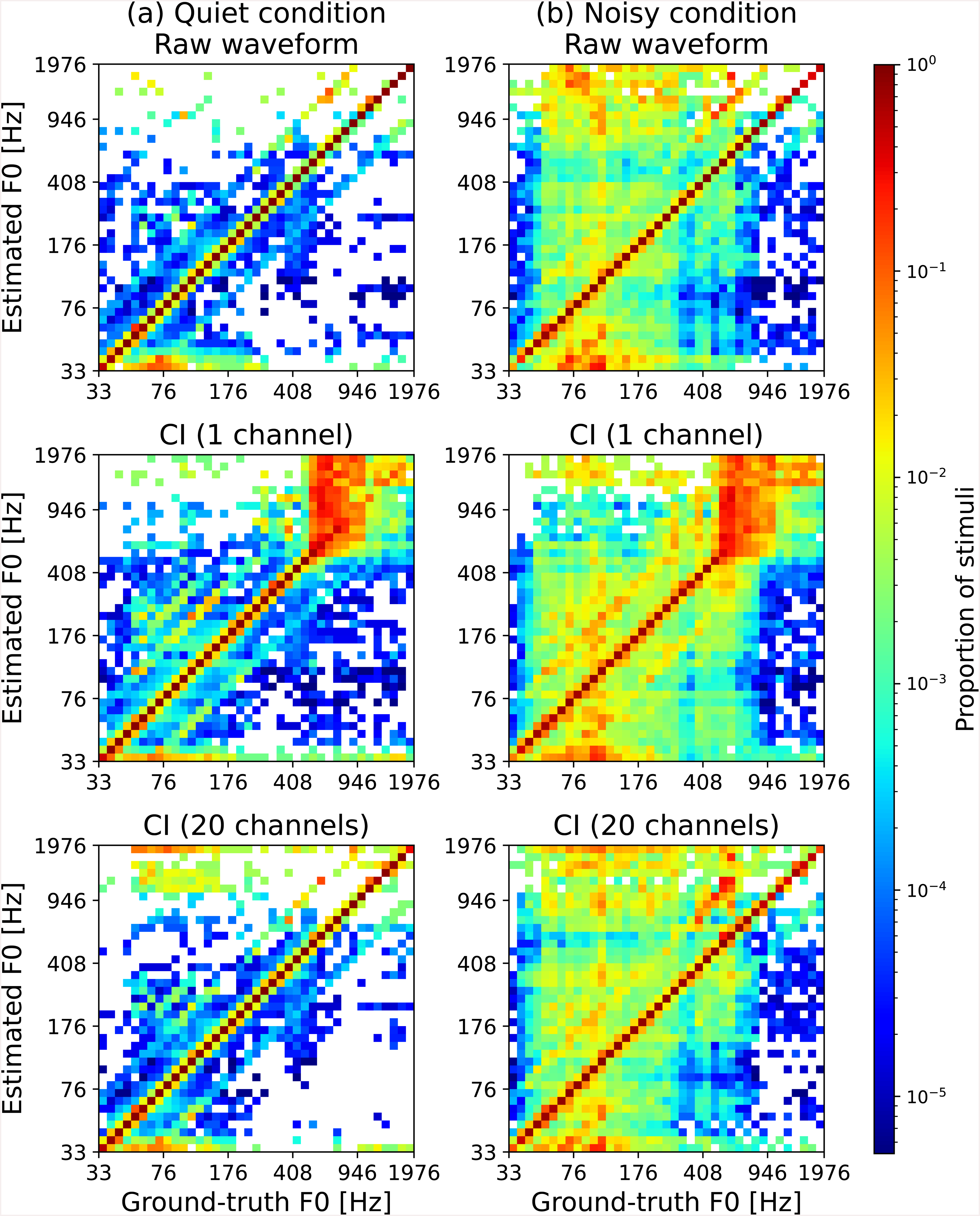
Confusion matrices between ground-truth F0 and estimated F0. Each column shows results under (a) quiet condition and (b) noisy condition. Top panels represent results for waveform model, while middle and bottom panels show matrices for CI model with 1 and 20 channels (both with pulse rate of 2,000 pps). Axes of all panels are on log scale. For easier identification of clusters with relatively lower counts, count represented as proportion is on log scale, and number of samples in each column was normalized to sum to one. Empty clusters indicate that count is zero. Note that this figure plots results of one of trained models with different random seeds.

Figure 7 summarizes the estimation errors (i.e., the difference from the ground truth), representing the mean absolute error (MAE) of F0. The analysis results were consistent with those on the percent correct described earlier: for all the configurations of the CI model, the degree of error under the quiet condition (Figure 7(a)) was smaller than that under the noisy condition (Figure 7(b)), confirming the distractive effect of background noise in general. The effect of the pulse rate was apparent, particularly under the noisy condition (i.e., smaller pulse rate resulting in larger MAE).

Figure 7.

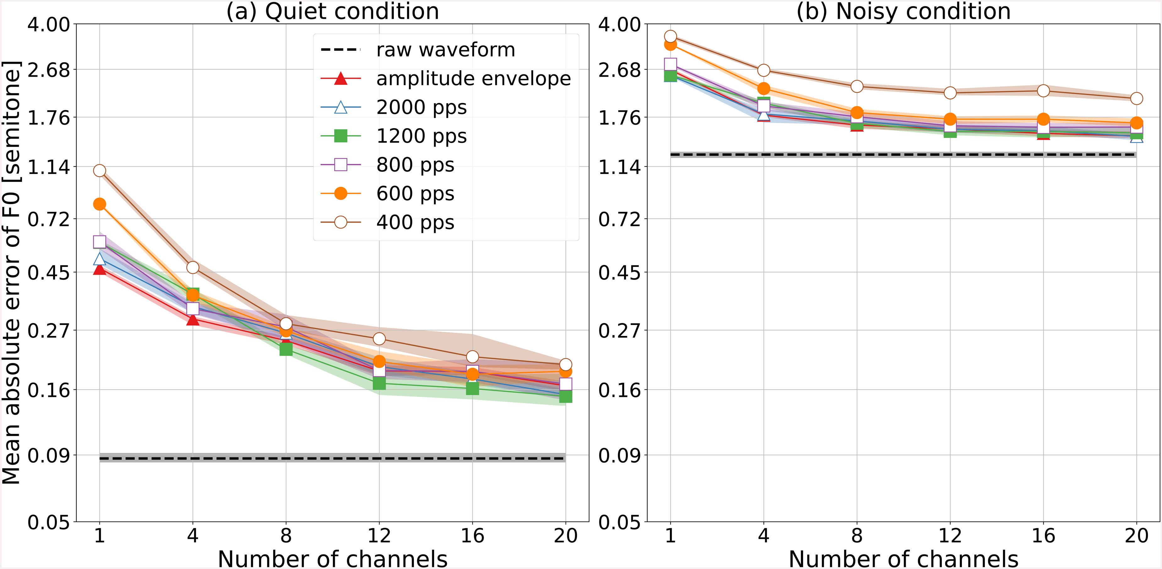
Mean absolute error (MAE) of F0 between predicted and ground-truth values in semitones on log scale under (a) quiet condition and (b) under noisy condition. Panels show MAE as function of number of channels of CI signal. Each line indicates differences in pulse rate, specifically 2,000, 1,200, 800, and 400 pps. Black-dashed line indicates MAE of waveform model. MAE shows mean of five networks initializing parameters with different random seeds, and shaded region shows 95% bootstrap confidence intervals of mean.

Relationship Between Performance and Signal-to-Noise Ratio

Section “Overall Accuracy of F0 Estimation” indicated that model performance was generally worse under noisy conditions than under quiet conditions, and this was true for both the waveform and CI models. We further explored the noise effect and examined how the SNR affected performance. To calculate the percent correct for each SNR condition, we randomly extracted 5,000 samples from the original clean test set and added noise samples, randomly extracted from JEIDA-NOISE, to them at levels ranging from 0 to 15 dB in 3-dB increments. In this process, the noise differed between samples but was the same across different dB conditions. We focused on the CI model configured with 2,000 pps and 20 or 1 channels. Figure 8 plots the percent correct as a function of SNR. To assess the effect of SNR on the performance of F0 estimation, we applied a linear mixed model (LMM) with SNR as a fixed effect and the F0-estimation model as a random effect. For each F0-estimation model, five networks were trained with initial parameters generated by different random seeds. The percent correct values were RAU-transformed and served as the response variables in the LMM. The LMM revealed a significant positive effect of SNR on the RAU-transformed percent correct (coefficient = 1.717, standard error = 0.030, P < .001), indicating that the performance varied significantly across SNR levels, with higher accuracy observed in high SNR conditions compared to low SNR conditions.

Figure 8.

Effect of noise intensity on model performance. This panel plots percent correct as function of SNR from 0 to 15 dB in increments of 3 dB. Red circles, blue triangles, and green squares indicate waveform model, CI model (2,000 pps, 20 channels), and CI model (2,000 pps, 1 channel), respectively. Percent correct shows mean of five networks initializing parameters with different random seeds, and shaded region shows 95% bootstrap confidence intervals of mean.

The three functions (i.e., the red, blue, and green lines) were generally parallel. To achieve a given percent correct (e.g., 90%), the CI model with 20 channels required about a 6-dB higher SNR than the waveform model. While the differences in the number of channels (place cues) affected the overall performance, there was no significant difference in the performance with respect to SNR (slope of each line).

Relationship Between F0 and Accuracy

The “Comparison of Ground-Truth and Estimation” section suggests that place cues, determined by the number of channels, play an important role in accurately estimating higher F0. We elaborated this by plotting percent correct as a function of ground-truth F0 for conditions with different numbers of channels (Figure 9). The line color represents each pulse rate. For each frequency range, we randomly sampled 2,000 instances per range to ensure an equal number of instances falling in each ground-truth F0 range for deriving the percent correct. For both quiet (Figure 9(a)) and noisy conditions (Figure 9(b)), poor place cues (i.e., conditions of using around 1 to 8 channels) degraded accuracy in the higher F0 range. However, accuracy in the lower F0 range, below approximately 300 Hz, was high, as it would provide sufficient temporal cues below the cut-off frequency of the low-pass filter.

Figure 9.

Performance of F0 estimation models (a) under quiet condition and (b) noisy condition. Panels show percent correct as function of ground-truth F0 range. Each line indicates differences in pulse rate, while each row represents channel. Percent correct shows mean of five networks initializing parameters with different random seeds, and shaded region shows 95% bootstrap confidence intervals of mean.

Impact of the Upper-Cut-Off Frequency of the Temporal Envelope Cues

We further investigated the effect of temporal envelope cues by investigating different cut-off frequencies of the low-pass filter used for envelope extraction, that is, 50, 100, 200, 300, and 600 Hz. The panels in Figures 10 and 11 are analogous to those in Figures 5 and 9, respectively, but controlling cut-off frequency instead of pulse rate. In this analysis, the pulse rate for all CI models was 2,000 pps. The overall performance illustrated in Figure 10 suggests that finer temporal cues provide better accuracy. At 600 Hz, which was higher than the commonly used 300 Hz, performance was comparable to those with raw waveforms. The greater the number of channels, the smaller the accuracy differences between the CI models with different cut-off frequencies. However, the poorest temporal-cue condition (50 Hz) showed significantly poorer performance, even in the finest place-cue condition (20 channels), compared with other models. The details of this accuracy are illustrated for each F0 range in Figure 11. From the results under the 1-channel condition in a quiet environment (Figure 11(a)), the accuracy was high when the F0 range was below the cut-off frequency, indicating that the cut-off frequency dictates the temporal cues necessary to accurately estimate F0. With a larger number of channels, accuracy improved, especially in the higher F0 range, as also shown in Figure 9. However, the performance of the CI model with a 50-Hz cut-off frequency (i.e., the temporal envelope cues are presented minimally) could not be fully compensated even with finer place cues (20 channels) within the 60- to 180-Hz ground-truth F0 range. Under noisy conditions (Figure 11(b)), the CI model with the lowest cut-off frequency demonstrated poor accuracy across all channels, even when the true F0 range was below 60 Hz.

Figure 10.

Performance of F0 estimation models (a) under quiet condition and (b) noisy condition. Panels show percent correct (top) and rationalized arcsine units (RAU) (bottom) as function of number of channels of CI signal. Each line indicates differences in cut-off frequency of low-pass filter. Pulse rate for all CI models is 2,000 pps. Black-dashed line indicates percent correct or RAU of waveform model. Each value shows mean of five networks initializing parameters with different random seeds, and shaded region shows 95% bootstrap confidence intervals of mean.

Figure 11.

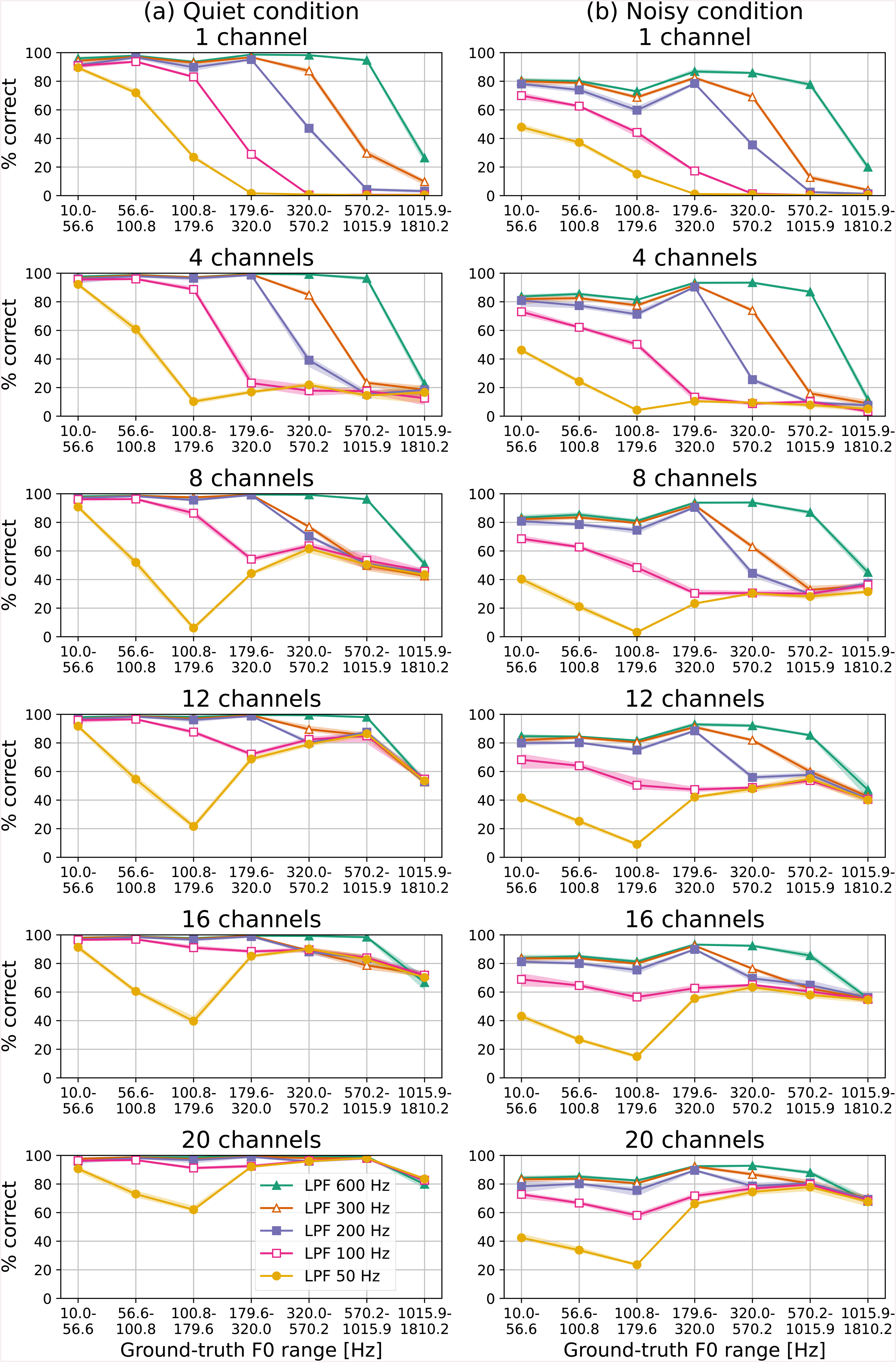
Performance of F0 estimation models (a) under quiet condition and (b) noisy condition. Panels show percent correct as function of ground-truth F0 range. Each line indicates differences in cut-off frequency of low-pass filter, while each row represents channel. Percent correct shows mean of five networks initializing parameters with different random seeds, and shaded region shows 95% bootstrap confidence intervals of mean.

Discussion

Previous studies have shown that a CI group was less accurate than a normal hearing group in a pitch-discrimination task, but some CI users were able to discriminate with high accuracy despite the degradation in the CI signal. This study was mainly motivated by those findings, and we systematically investigated the upper limit of the amount of F0 information contained in the CI signal, along with the effect of the number of channels and pulse rate. The results under the quiet condition indicate that the CI signal had sufficient information for estimating the F0 with a certain number of channels. In contrast, under the noisy condition, it was difficult to estimate F0 from the CI signal, and the performance gap between the CI and waveform models was greater than that under the quiet condition. As expected, there was a clear correlation between the SNR and F0-estimation performance.

In the quiet condition, the CI signal contained substantial F0 information under conditions where the pulse signals were generated with almost 8 channels regardless of the pulse rate (Figure 5(a)). Thanks to the introduction of multi-channel CI devices, around 8 channels are practical for any manufacturer (Zeng et al., 2008). Moreover, our results indicate that increasing the number of channels to 8 or more further improves F0 estimation. This is comparable to recent studies (Berg et al., 2019; Croghan et al., 2017), which demonstrated that speech intelligibility improved with more than 7 to 10 channels. On the other hand, some studies have shown that increasing the number of electrodes beyond 7 to 10 channels does not necessarily improve speech performance under both quiet and noisy conditions (Fishman et al., 1997; Friesen et al., 2001). These discrepancies highlight the need for further investigation to better understand the relationship between the number of channels and auditory outcomes. The CI models were also able to estimate F0 with an MAE within a fraction of a semitone under quiet conditions (Figure 7(a)). From the above findings, current CI users may in principle exhibit higher pitch perception, no matter what device they use. In fact, a previous study (Nimmons et al., 2008) has shown that some CI users could identify one-semitone difference in a pitch-discrimination task. Therefore, the results under the quiet condition suggest that the main reason for the deterioration in the pitch sensitivity of CI users is due to neuroplasticity of relevant brain areas induced by auditory experience or implantation age, along with other patient-oriented and/or surgical-oriented factors such as neural survival, and insertion depth of electrode array, rather than device-oriented factors.

Contrary to the results under the quiet condition, the difficulty of F0 estimation was demonstrated under noisy conditions (Figure 5(b)). This was consistent with previous studies showing that CI listeners had not fully recovered their hearing ability under noisy conditions compared with normal-hearing listeners. For example, a scoping review (Boisvert et al., 2020) summarized an almost 30% performance gap in a sentence-recognition task under a noisy condition compared with under a quiet condition. The main reasons for this negative impact were the vulnerability of the temporal envelope against interference sounds and the absence of a temporal fine structure (TFS) in the CI signal, which was impaired in the process of deriving the envelope from the raw waveform (Moore, 2019). The TFS cue has played a critical role in perceiving speech in the presence of competing sounds through experiments on normal-hearing listeners by using a vocoded signal in English (Hopkins & Moore, 2010) and in Mandarin (Kong & Zeng, 2006). In fact, the Env model (i.e., received an amplitude envelope as input) performed significantly poorer than the waveform model (Figures 5(b) and 7(b)). Nevertheless, there is no compelling evidence that adding TFS cues helps CI users’ perception, and this topic remains a subject of ongoing debate (Carlyon & Goehring, 2021; Wouters et al., 2015).

The performance differences within CI model versions were relatively slight for 8 or more channels compared with fewer channels, regardless of pulse rate under the quiet condition or over 600 pps under the noisy condition. It seems that with a limited number of channels (<8 channels), the place cue became unreliable, prompting reliance on the temporal cue. Similarly, with a low pulse rate (<600 or 800 pps), the temporal cue was unreliable, leading to reduced accuracy. The tendency led to the importance of combining the place cues and rate of stimulation (or temporal cues), as shown in previous CI studies (Bissmeyer & Goldsworthy, 2022; Erfanian Saeedi et al., 2017; Luo et al., 2012). We can interpret the present data as indicating that the contemporary CI configuration, with over 600 or 800 pps and more than 8 channels, is near optimal for the purpose of extracting F0 information from the envelope.

To determine model performance with actual listeners in a realistic noise environment, we should examine a wide range of environmental sounds as the background noise. The current study involved using one class of environmental sounds, that is, real-recorded sounds, which had essentially no harmonic structure, hence, no F0 information. Future studies may include other types of noise with a certain amount of F0 information, which would compete with the target F0.

We also recognize that the simulations of CI signals used in the present study did not sufficiently cover the properties of modern CI devices currently available. Factors that can affect the performance include the bandwidth or filter-shape configurations of the band-pass filter, characteristics of the microphone, automatic gain control, and other signal processing functions. We also simulated a CIS strategy, but did not test, for example, the fine structure processing strategy (Wilson & Dorman, 2008; Wilson et al., 2005; Wouters et al., 2015), which was proposed for better music appreciation (Müller et al., 2012). Nevertheless, the contribution of the present paper is demonstrating the significance of directly extracting F0 information using DNNs from the basic pulsatile CI signal. Future studies may take advantage of this approach as a tool for evaluating the benefits of various parameters and strategies including n-of-m strategies such as used in the Cochlear make of CI.

Another concern is that our approach did not explicitly incorporate auditory neural representations of CI users into the model. For example, a previous study (Saddler et al., 2021) used simulated auditory nerve representations as the input to DNN models to develop a model of pitch perception. Another DNN study (Brochier et al., 2022) used neural excitation patterns converted from CI device outputs to predict speech perception of CI. For this study, the pulsatile signal derived from CI processors was applied to DNN models to determine whether the primary cause of the deterioration in CI users’ pitch sensitivity is the CI signal, rather than biological, patient-specific, or surgical factors. Future studies may include the simulation of auditory nerve responses to acoustic stimuli to investigate the effects of channel interaction, neural survival, and electrode-array insertion depth.

The analyses under noisy conditions (400 pps of the pulse rate in Figure 5(b)) further revealed the importance of the resolution of the temporal envelope information determined from the pulse rate of CI signals. The effect of varying the pulse rate has been explored in several studies (Arora, 2012; Arora et al., 2009; Fu & Shannon, 2000; Loizou et al., 2000; Shannon et al., 2011). The study by Arora (2012), for example, has shown that CI users improved their speech recognition, especially under noisy condition, as the pulse rate increased to about 500 pps per channel. Our analyses indicate that under the quiet condition (Figure 5(a)), the signal with 400 pps and 8 channels would be sufficient for the CI model to achieve the same performance as that of an Env model (regarded as the condition of no information loss by temporal sampling). Under the noisy condition (Figure 5(b)), however, the same input was not sufficient to reach the Env model's performance, even though the signal with 800 pps and the 8 channels would be sufficient. While our results indicate that increasing the pulse rate generally led to performance improvements, the speech perception of CI users does not consistently improve with higher pulse rates and can sometimes even worsen (Brochier et al., 2017). Therefore, future work may include considering factors such as between-channel interactions induced by high pulse rates (Boulet et al., 2016).

It is important to point out that actual CI listeners do not always take advantage of high pulse rates in pitch discrimination on the basis of temporal information, which has been demonstrated in several earlier studies. For example, when the stimuli were simple pulse trains, in which a higher pulse rate is expected to evoke a higher pitch percept, most CI users exhibited difficulty in discriminating the pulse rate with a baseline pulse rate above approximately 300 pps, which is much smaller than a normal hearing listener (Carlyon et al., 2010; Moore & Carlyon, 2005; Vandali et al., 2013; Venter & Hanekom, 2014; Zeng, 2002; Zhou et al., 2019). We should note that it is difficult to determine the “true” upper-bound pulse rate: The task performance varied considerably among CI users (some are able to detect rate changes around 700 or 1,000 pps; Kong & Carlyon, 2010; Townshend et al., 1987). Furthermore, the upper limit of pulse rate discrimination may also change due to improvements brought by perceptual learning (Bissmeyer et al., 2020; Goldsworthy & Shannon, 2014), although these improvements may stem from procedural or task-specific factors, such as an increased understanding of the task requirements or perhaps picking up on extraneous cues specific to the experiment, limiting their generalizability to real-life situations. Another form of temporal information that could be associated with pitch perception is the amplitude envelope as a modulator of the pulse train. Studies that assessed the detection or discrimination of the amplitude envelope with various pulse rates (Fraser & McKay, 2012; Galvin & Fu, 2005; Green et al., 2012; Pfingst et al., 2007) indicate that increased pulse rates of the pulse train could induce no effect or even degraded performance under conditions such as exceptionally high carrier rate (e.g., 4,000 pps) or reduction in the level of carrier.

As shown in Figures 9, 10, and 11, we examined the interplay between the fidelity of place-of-excitation and temporal cues with the F0 range by varying the number of channels and pulse rate or cut-off frequency for envelope extraction. The results indicate that accurate estimation of low F0 was possible even in the absence of place cues (i.e., with just one channel) and that the cut-off frequency affected the estimable low F0 range, highlighting the importance of temporal-envelope-cue fidelity. Conversely, estimating higher F0 required a certain number of channels, indicating the contribution of place cues. This aligns with previous studies, which demonstrated that the number of channels affects the accuracy of melody perception at high F0 ranges (from 414 to 1,046 Hz; primarily place cues) (Singh et al., 2009). As shown in Figure 3, these tendencies are somewhat natural, as a CI signal can provide strong temporal cues for low F0 and strong place cues but no timing cues for high F0. We also observed a similar trend in the F0 tracking results shown in Figure 4. Even when temporal cues had very limited fidelity (e.g., the LPF 50-Hz condition in Figure 11, where LPF denotes low-pass filter), performance at high F0 was well compensated by increasing the number of channels. Several studies of CI users explored the contributions of place and temporal pitch for melody recognition using different F0 ranges comprised of pure or harmonic tones (Singh et al., 2009; Swanson et al., 2019). While different studies reported varying performances between F0 ranges, possibly due to differences in stimulus composition (e.g., harmonic composition), our CI model with sufficient temporal and place cues demonstrated almost no differences and achieved nearly perfect performance under quiet conditions.

It is interesting that the CI models with more than a certain number of channels and pulse rates achieved almost perfect accuracy in estimating the F0 under quiet condition, while a previous study (Erfanian Saeedi et al., 2017) demonstrated only slight, better-than-chance performance, also under quiet condition. One possible reason for the marked difference between the studies is the difference in the model structure. The model in the previous study had a single feed-forward layer with pre-extracted features, while the CI model is capable of acquiring more complex expressions in “raw” signals. We trained models with a much larger amount of data than previous studies, as typical for DNN models. Another factor could be differences in the input signals to the model. The previous study used the across-time average of the cochleogram as a place cue and inter-spike-interval histogram as a temporal cue, while we used the two-dimensional pulsatile CI signal for the model input. The CI model could have acquired latent features other than the above two cues. For example, when the temporal cues had been extracted, all spikes were integrated between channels to calculate input features, presumably leading to the loss of temporal cues per channel. However, a previous biologically-motivated modeling study (Shamma & Dutta, 2019) has shown that the processing procedure of an unresolved pitch would differ from a resolved pitch in the temporal axis. The CI model may have implicitly enabled such different processing between channels. We hope that future studies exploring the detailed internal representations of a DNN model (Adadi & Berrada, 2018; Arrieta et al., 2020) will reveal specific cues and processing strategies to take advantage of the latent features in CI signals.

Supplemental Material

sj-docx-1-tia-10.1177_23312165241298606 - Supplemental material for Estimating Pitch Information From Simulated Cochlear Implant Signals With Deep Neural Networks

Supplemental material, sj-docx-1-tia-10.1177_23312165241298606 for Estimating Pitch Information From Simulated Cochlear Implant Signals With Deep Neural Networks by Takanori Ashihara, Shigeto Furukawa and Makio Kashino in Trends in Hearing

Footnotes

Declaration of Conflicting Interests

The authors declared no potential conflicts of interest with respect to the research, authorship, and/or publication of this article.

Funding

The authors disclosed receipt of the following financial support for the research, authorship, and/or publication of this article: This work was supported by the Japan Society for the Promotion of Science (grant number JP23H01063).

ORCID iD

Shigeto Furukawa

Supplemental Material

Supplemental material for this paper is available online.

Notes

References

Adadi

Berrada

(2018). Peeking inside the black-box: A survey on explainable artificial intelligence (XAI). IEEE Access, 6, 52138–52160. https://doi.org/10.1109/ACCESS.2018.2870052

Arora

(2012). Cochlear implant stimulation rates and speech perception. In Ramakrishnan

(Ed.), Modern speech recognition. IntechOpen. https://doi.org/10.5772/49992

Arora

Dawson

Dowell

Vandali

(2009). Electrical stimulation rate effects on speech perception in cochlear implants. International Journal of Audiology, 48(8), 561–567. https://doi.org/10.1080/14992020902858967

Arrieta

A. B.

Díaz-Rodríguez

Del Ser

Bennetot

Tabik

Barbado

Garcia

Gil-Lopez

Molina

Benjamins

Chatila

Herrera

(2020). Explainable artificial intelligence (XAI): Concepts, taxonomies, opportunities and challenges toward responsible AI. Information Fusion, 58, 82–115. https://doi.org/10.1016/j.inffus.2019.12.012

Berg

K. A.

Noble

J. H.

Dawant

B. M.

Dwyer

R. T.

Labadie

R. F.

Gifford

R. H.

(2019). Speech recognition as a function of the number of channels in perimodiolar electrode recipients. The Journal of the Acoustical Society of America, 145(3), 1556–1564. https://doi.org/10.1121/1.5092350

Bissmeyer

S. R. S.

Goldsworthy

R. L.

(2022). Combining place and rate of stimulation improves frequency discrimination in cochlear implant users. Hearing Research, 424, 108583. https://doi.org/10.1016/j.heares.2022.108583

Bissmeyer

S. R. S.

Hossain

Goldsworthy

R. L.

(2020). Perceptual learning of pitch provided by cochlear implant stimulation rate. PLOS One, 15(12), e0242842. https://doi.org/10.1371/journal.pone.0242842

Bittner

R. M.

McFee

Salamon

Bello

J. P.

(2017). Deep salience representations for F0 estimation in polyphonic music. International Society for Music Information Retrieval Conference, 63–70.

Boisvert

Reis

Cowan

Dowell

R. C.

(2020). Cochlear implantation outcomes in adults: A scoping review. PLOS ONE, 15(5), 1–26. https://doi.org/10.1371/journal.pone.0232421

10.

Boulet

White

Bruce

I. C.

(2016). Temporal considerations for stimulating spiral ganglion neurons with cochlear implants. Journal of the Association for Research in Otolaryngology : JARO, 17(1), 1–17. https://doi.org/10.1007/s10162-015-0545-5

11.

Brochier

McDermott

H. J.

McKay

C. M.

(2017). The effect of presentation level and stimulation rate on speech perception and modulation detection for cochlear implant users. The Journal of the Acoustical Society of America, 141(6), 4097. https://doi.org/10.1121/1.4983658

12.

Brochier

Schlittenlacher

Roberts

Goehring

Jiang

Vickers

Bance

(2022). From microphone to phoneme: An end-to-end computational neural model for predicting speech perception with cochlear implants. IEEE Transactions on Biomedical Engineering, 69(11), 3300–3312. https://doi.org/10.1109/TBME.2022.3167113

13.

Carlyon

R. P.

Deeks

J. M.

McKay

C. M.

(2010). The upper limit of temporal pitch for cochlear-implant listeners: Stimulus duration, conditioner pulses, and the number of electrodes stimulated. The Journal of the Acoustical Society of America, 127(3), 1469–1478. https://doi.org/10.1121/1.3291981

14.

Carlyon

R. P.

Goehring

(2021). Cochlear implant research and development in the twenty-first century: A critical update. Journal of the Association for Research in Otolaryngology, 22(5), 481–508. https://doi.org/10.1007/s10162-021-00811-5

15.

Clark

G. M.

(2015). The multi-channel cochlear implant: Multi-disciplinary development of electrical stimulation of the cochlea and the resulting clinical benefit. Hearing Research, 322, 4–13. https://doi.org/10.1016/j.heares.2014.08.002

16.

Crew

J. D.

Galvin

J. J.

(2012). Channel interaction limits melodic pitch perception in simulated cochlear implants. The Journal of the Acoustical Society of America, 132(5), 429–435. https://doi.org/10.1121/1.4758770

17.

Croghan

N. B. H.

Duran

S. I.

Smith

Z. M.

(2017). Re-examining the relationship between number of cochlear implant channels and maximal speech intelligibility. The Journal of the Acoustical Society of America, 142(6), EL537. https://doi.org/10.1121/1.5016044

18.

Dorman

M. F.

Loiselle

L. H.

Cook

S. J.

Yost

W. A.

Gifford

R. H.

(2016). Sound source localization by normal-hearing listeners, hearing-impaired listeners and cochlear implant listeners. Audiology and Neurotology, 21(3), 127–131. https://doi.org/10.1159/000444740

19.

Drennan

W. R.

Rubinstein

J. T.

(2008). Music perception in cochlear implant users and its relationship with psychophysical capabilities. Journal of Rehabilitation Research and Development, 45(5), 779–789. https://doi.org/10.1682/jrrd.2007.08.0118

20.

Duan

Pardo

Zhang

(2010). Multiple fundamental frequency estimation by modeling spectral peaks and non-peak regions. IEEE Transactions on Audio, Speech, and Language Processing, 18(8), 2121–2133. https://doi.org/10.1109/TASL.2010.2042119

21.

Engel

Resnick

Roberts

Dieleman

Norouzi

Eck

Simonyan

(2017). Neural audio synthesis of musical notes with WaveNet autoencoders. In Proceedings of the 34th International Conference on Machine Learning (ICML), 1068–1077. https://proceedings.mlr.press/v70/engel17a.html

22.

Erfanian Saeedi

Blamey

P. J.

Burkitt

A. N.

Grayden

D. B.

(2014). Application of a pitch perception model to investigate the effect of stimulation field spread on the pitch ranking abilities of cochlear implant recipients. Hearing Research, 316, 129–137. https://doi.org/10.1016/j.heares.2014.08.006

23.

Erfanian Saeedi

Blamey

P. J.

Burkitt

A. N.

Grayden

D. B.

(2017). An integrated model of pitch perception incorporating place and temporal pitch codes with application to cochlear implant research. Hearing Research, 344, 135–147. https://doi.org/10.1016/j.heares.2016.11.005

24.

Fishman

K. E.

Shannon

R. V.

Slattery

W. H.

(1997). Speech recognition as a function of the number of electrodes used in the SPEAK cochlear implant speech processor. Journal of Speech, Language, and Hearing Research, 40(5), 1201–1215. https://doi.org/10.1044/jslhr.4005.1201

25.

Fraser

McKay

C. M.

(2012). Temporal modulation transfer functions in cochlear implantees using a method that limits overall loudness cues. Hearing Research, 283(1–2), 59–69. https://doi.org/10.1016/j.heares.2011.11.009

26.

Friesen

L. M.

Shannon

R. V.

Baskent

Wang

(2001). Speech recognition in noise as a function of the number of spectral channels: Comparison of acoustic hearing and cochlear implants. The Journal of the Acoustical Society of America, 110(2), 1150–1163. https://doi.org/10.1121/1.1381538

27.

Q. J.

Shannon

R. V.

(1998). Effects of amplitude nonlinearity on phoneme recognition by cochlear implant users and normal-hearing listeners. The Journal of the Acoustical Society of America, 104(5), 2570–2577. https://doi.org/10.1121/1.423912

28.

Q. J.

Shannon

R. V.

(2000). Effect of stimulation rate on phoneme recognition by nucleus-22 cochlear implant listeners. The Journal of the Acoustical Society of America, 107(1), 589–597. https://doi.org/10.1121/1.428325

29.

Galvin

J. J.

Q. J.

(2005). Effects of stimulation rate, mode and level on modulation detection by cochlear implant users. Journal of the Association for Research in Otolaryngology, 6, 269–279. https://doi.org/10.1007/s10162-005-0007-6

30.

Geurts

Wouters

(2001). Coding of the fundamental frequency in continuous interleaved sampling processors for cochlear implants. The Journal of the Acoustical Society of America, 109(2), 713–726. https://doi.org/10.1121/1.1340650

31.

Gfeller

Turner

Mehr

Woodworth

Fearn

Knutson

J. F.

Witt

Stordahl

(2002). Recognition of familiar melodies by adult cochlear implant recipients and normal-hearing adults. Cochlear Implants International, 3(1), 29–53. https://doi.org/10.1179/cim.2002.3.1.29

32.

Goldsworthy

R. L.

Shannon

R. V.

(2014). Training improves cochlear implant rate discrimination on a psychophysical task. The Journal of the Acoustical Society of America, 135(1), 334–341. https://doi.org/10.1121/1.4835735

33.

Green

Faulkner

Rosen

(2012). Variations in carrier pulse rate and the perception of amplitude modulation in cochlear implant users. Ear and Hearing, 33(2), 221–230. https://doi.org/10.1097/AUD.0b013e318230fff8

34.

Hopkins

Moore

B. C. J.

(2010). The importance of temporal fine structure information in speech at different spectral regions for normal-hearing and hearing-impaired subjects. The Journal of the Acoustical Society of America, 127(3), 1595–1608. https://doi.org/10.1121/1.3293003

35.

Itahashi

(1990). Recent speech database projects in Japan. In International Conference on Spoken Language Processing (ICSLP), pp. 1081–1084.

36.

Kang

Liu

Drennan

Longnion

Ruffin

Nie

Won

Worman

Yueh

Rubinstein

(2009). Development and validation of the University of Washington Clinical Assessment of Music Perception test. Ear and Hearing, 30(4), 411–418. https://doi.org/10.1097/AUD.0b013e3181a61bc0

37.

Kenway

Tam

Y. C.

Vanat

Harris

Gray

Birchall

Carlyon

Axon

(2015). Pitch discrimination: An independent factor in cochlear implant performance outcomes. Otology & Neurotology, 36(9), 1472–1479. https://doi.org/10.1097/MAO.0000000000000845

38.

Kim

J. W.

Salamon

Bello

J. P.

(2018). CREPE: A convolutional representation for pitch estimation. In IEEE International Conference on Acoustics, Speech and Signal Processing (ICASSP), 161–165, https://doi.org/10.1109/ICASSP.2018.8461329

39.

Kong

Y. Y.

Carlyon

R. P.

(2010). Temporal pitch perception at high rates in cochlear implants. The Journal of the Acoustical Society of America, 127(5), 3114–3123. https://doi.org/10.1121/1.3372713

40.

Kong

Y.-Y.

Cruz

Jones

J. A.

Zeng

F.-G.

(2004). Music perception with temporal cues in acoustic and electric hearing. Ear and Hearing, 25(2), 173–185. https://doi.org/10.1097/01.aud.0000120365.97792.2f

41.

Kong

Y.-Y.

Zeng

F.-G.

(2006). Temporal and spectral cues in Mandarin tone recognition. The Journal of the Acoustical Society of America, 120(5), 2830–2840. https://doi.org/10.1121/1.2346009

42.

Kral

Sharma

(2012). Developmental neuroplasticity after cochlear implantation. Trends in Neurosciences, 35(2), 111–122. https://doi.org/10.1016/j.tins.2011.09.004

43.

Limb

C. J.

Roy

A. T.

(2014). Technological, biological, and acoustical constraints to music perception in cochlear implant users. Hearing Research, 308, 13–26. https://doi.org/10.1016/j.heares.2013.04.009

44.

Loizou

(1998). Mimicking the human ear. IEEE Signal Processing Magazine, 15(5), 101–130. https://doi.org/10.1109/79.708543

45.

Loizou

(1999). Signal-processing techniques for cochlear implants. IEEE Engineering in Medicine and Biology Magazine, 18(3), 34–46. https://doi.org/10.1109/51.765187

46.

Loizou

P. C.

(2006). Speech processing in vocoder-centric cochlear implants. Advances in Oto-Rhino-Laryngology, 64, 109–143. https://doi.org/10.1159/000094648

47.

Loizou

P. C.

Poroy

Dorman

(2000). The effect of parametric variations of cochlear implant processors on speech understanding. The Journal of the Acoustical Society of America, 108(2), 790–802. https://doi.org/10.1121/1.429612

48.

Looi

McDermott

McKay

Hickson

(2004). Pitch discrimination and melody recognition by cochlear implant users. International Congress Series, 1273, 197–200. https://doi.org/10.1016/j.ics.2004.08.038

49.

Luo

Padilla

Landsberger

D. M.

(2012). Pitch contour identification with combined place and temporal cues using cochlear implants. The Journal of the Acoustical Society of America, 131(2), 1325–1336. https://doi.org/10.1121/1.3672708

50.

McDermott

H. J.

(2004). Music perception with cochlear implants: A review. Trends in Amplification, 8(2), 49–82. https://doi.org/10.1177/108471380400800203

51.

McDermott

J. H.

Oxenham

A. J.

(2008). Music perception, pitch, and the auditory system. Current Opinion in Neurobiology, 18(4), 452–463. https://doi.org/10.1016/j.conb.2008.09.005

52.

Mehta

A. H.

Oxenham

A. J.

(2017). Vocoder simulations explain complex pitch perception limitations experienced by cochlear implant users. Journal of the Association for Research in Otolaryngology, 18(6), 789–802. https://doi.org/10.1007/s10162-017-0632-x

53.

Moore

B. C. J.

(2019). The roles of temporal envelope and fine structure information in auditory perception. Acoustical Science and Technology, 40(2), 61–83. https://doi.org/10.1250/ast.40.61

54.

Moore

B. C. J.

Carlyon

R. P.

(2005). Perception of pitch by people with cochlear hearing loss and by cochlear implant users. In Pitch. Springer Handbook of Auditory Research (Vol. 24). Springer. https://doi.org/10.1007/0-387-28958-5_7

55.

Müller

Brill

Hagen

Moeltner

Brockmeier

S. J.

Stark

Helbig

Maurer

Zahnert

Zierhofer

Nopp

Anderson

(2012). Clinical trial results with the MED-EL fine structure processing coding strategy in experienced cochlear implant users. ORL; Journal for Oto-Rhino-Laryngology and its Related Specialties, 74(4), 185–198. https://doi.org/10.1159/000337089

56.

Nagels

Gaudrain

Vickers

Hendriks

Başkent

(2024). Prelingually deaf children with cochlear implants show better perception of voice cues and speech in competing speech than postlingually deaf adults with cochlear implants. Ear and Hearing, 45(4), 952–968. https://doi.org/10.1097/AUD.0000000000001489

57.

Naik

A. N.

Varadarajan

V. V.

Malhotra

P. S.

(2021). Early pediatric cochlear implantation: An update. Laryngoscope Investigative Otolaryngology, 6(3), 512–521. https://doi.org/10.1002/lio2.574

58.

Nicholas

Geers

(2007). Will they catch up? The role of age at cochlear implantation in the spoken language development of children with severe to profound hearing loss. Journal of Speech, Language, and Hearing Research (JSLHR), 50(4), 1048–1062. https://doi.org/10.1044/1092-4388(2007/073)

59.

Nikolopoulos

T. P.

O’Donoghue

G. M.

Archbold

(1999). Age at implantation: Its importance in pediatric cochlear implantation. The Laryngoscope, 109(4), 595–599. https://doi.org/10.1097/00005537-199904000-00014

60.

Nimmons

G. L.

Kang

R. S.

Drennan

W. R.

Longnion

Ruffin

Worman

Yueh

Rubinstein

J. T.

(2008). Clinical assessment of music perception in cochlear implant listeners. Otology & Neurotology, 29(2), 149–155. https://doi.org/10.1097/mao.0b013e31812f7244

61.

Niparko

J. K.

Tobey

E. A.

Thal

D. J.

Eisenberg

L. S.

Wang

N.-Y.

Quittner

A. L.

Fink

N. E.

& CDaCI Investigative Team (2010). Spoken language development in children following cochlear implantation. JAMA, 303(15), 1498–1506. https://doi.org/10.1001/jama.2010.451

62.

Oxenham

A. J.

(2008). Pitch perception and auditory stream segregation: Implications for hearing loss and cochlear implants. Trends in Amplification, 12(4), 316–331. https://doi.org/10.1177/1084713808325881

63.

Oxenham

A. J.

(2012). Pitch perception. Journal of Neuroscience, 32(39), 13335–13338. https://doi.org/10.1523/JNEUROSCI.3815-12.2012

64.

Peterson

N. R.

Pisoni

D. B.

Miyamoto

R. T.

(2010). Cochlear implants and spoken language processing abilities: Review and assessment of the literature. Restorative Neurology and Neuroscience, 28(2), 237–250. https://doi.org/10.3233/RNN-2010-0535

65.

Pfingst

B. E.

Thompson

C. S.

(2007). Effects of carrier pulse rate and stimulation site on modulation detection by subjects with cochlear implants. The Journal of the Acoustical Society of America, 121(4), 2236–2246. https://doi.org/10.1121/1.2537501

66.

Ping

Yuan

Feng

(2012). Musical pitch discrimination by cochlear implant users. Annals of Otology, Rhinology & Laryngology, 121(5), 328–336. https://doi.org/10.1177/000348941212100508

67.

Prevoteau

Chen

S. Y.

Lalwani

A. K.

(2018). Music enjoyment with cochlear implantation. Auris, Nasus, Larynx, 45(5), 895–902. https://doi.org/10.1016/j.anl.2017.11.008

68.

Saddler

M. R.

Gonzalez

McDermott

J. H.

(2021). Deep neural network models reveal interplay of peripheral coding and stimulus statistics in pitch perception. Nature Communications, 12, 7278. https://doi.org/10.1038/s41467-021-27366-6

69.

Salamon

Bittner

Bonada

Bosch

Gomez

Bello

(2017). An analysis/synthesis framework for automatic F0 annotation of multitrack datasets. Proceedings of the 18th International Society for Music Information Retrieval Conference (ISMIR), 71–78.

70.

Salamon

Gomez

Ellis

D. P. W.

Richard

(2014). Melody extraction from polyphonic music signals: Approaches, applications, and challenges. IEEE Signal Processing Magazine, 31(2), 118–134. https://doi.org/10.1109/MSP.2013.2271648

71.

Shamma

Dutta

(2019). Spectro-temporal templates unify the pitch percepts of resolved and unresolved harmonics. The Journal of the Acoustical Society of America, 145(2), 615–629. https://doi.org/10.1121/1.5088504

72.

Shannon

R. V.

Cruz

R. J.

Galvin

J. J.

(2011). Effect of stimulation rate on cochlear implant users’ phoneme, word and sentence recognition in quiet and in noise. Audiology and Neurotology, 16(2), 113–123. https://doi.org/10.1159/000315115

73.

Shannon

R. V.

Zeng

F.-G.

Kamath

Wygonski

Ekelid

(1995). Speech recognition with primarily temporal cues. Science, 270(5234), 303–304. https://doi.org/10.1126/science.270.5234.303

74.

Singh

Kong

Y. Y.

Zeng

F. G.

(2009). Cochlear implant melody recognition as a function of melody frequency range, harmonicity, and number of electrodes. Ear and Hearing, 30(2), 160–168. https://doi.org/10.1097/AUD.0b013e31819342b9

75.

Smeds

Wolters

Rung

(2015). Estimation of signal-to-noise ratios in realistic sound scenarios. Journal of the American Academy of Audiology, 26(02), 183–196. https://doi.org/10.3766/jaaa.26.2.7

76.

Studebaker

G. A.

(1985). A “rationalized” arcsine transform. Journal of Speech and Hearing Research, 28(3), 455–462. https://doi.org/10.1044/jshr.2803.455

77.

Sucher

C. M.

McDermott

H. J.

(2007). Pitch ranking of complex tones by normally hearing subjects and cochlear implant users. Hearing Research, 230(1), 80–87. https://doi.org/10.1016/j.heares.2007.05.002

78.

Swanson

B. A.

Marimuthu

V. M. R.

Mannell

R. H.

(2019). Place and temporal cues in cochlear implant pitch and melody perception. Frontiers in Neuroscience, 13, 1266. https://doi.org/10.3389/fnins.2019.01266

79.

Townshend

Cotter

Van Compernolle

White

R. L.

(1987). Pitch perception by cochlear implant subjects. The Journal of the Acoustical Society of America, 82(1), 106–115. https://doi.org/10.1121/1.395554

80.

Vandali

A. E.

Sly

Cowan

van Hoesel

R. J. M.

(2013). Pitch and loudness matching of unmodulated and modulated stimuli in cochlear implantees. Hearing Research, 302, 32–49. https://doi.org/10.1016/j.heares.2013.05.004

81.

Vandali

A. E.

Sucher

Tsang

D. J.

McKay

C. M.

Chew

J. W. D.

McDermott

H. J.

(2005). Pitch ranking ability of cochlear implant recipients: A comparison of sound-processing strategies. The Journal of the Acoustical Society of America, 117(5), 3126–3138. https://doi.org/10.1121/1.1874632

82.

Vandali

A. E.

Whitford

L. A.

Plant

K. L.

Clark

G. M.

(2000). Speech perception as a function of electrical stimulation rate: Using the nucleus 24 cochlear implant system. Ear and Hearing, 21(6), 608–624. https://doi.org/10.1097/00003446-200012000-00008

83.

Venter

P. J.

Hanekom

J. J.

(2014). Is there a fundamental 300Hz limit to pulse rate discrimination in cochlear implants? Journal of the Association for Research in Otolaryngology : JARO, 15(5), 849–866. https://doi.org/doi.:10.1007/s10162-014-0468-6

84.

Verschuur

C. A.

Lutman

M. E.

Ramsden

Greenham

O’Driscoll

(2005). Auditory localization abilities in bilateral cochlear implant recipients. Otology & Neurotology, 26(5), 965–971. https://doi.org/10.1097/01.mao.0000185073.81070.07

85.

Wilson

B. S.

(2015). Getting a decent (but sparse) signal to the brain for users of cochlear implants. Hearing Research, 322, 24–38. https://doi.org/10.1016/j.heares.2014.11.009

86.

Wilson

B. S.

Dorman

M. F.

(2008). Cochlear implants: A remarkable past and a brilliant future. Hearing Research, 242(1), 3–21. https://doi.org/10.1016/j.heares.2008.06.005

87.

Wilson

B. S.

Finley

C. C.

Lawson

D. T.

Wolford

R. D.

Eddington

D. K.

Rabinowitz

W. M.

(1991). Better speech recognition with cochlear implants. Nature, 352(6332), 236–238. https://doi.org/10.1038/352236a0

88.

Wilson

B. S.

Schatzer

Lopez-Poveda

E. A.

Sun

Lawson

D. T.

Wolford

R. D.

(2005). Two new directions in speech processor design for cochlear implants. Ear and Hearing, 26(4 Suppl), 73S–81S. https://doi.org/10.1097/00003446-200508001-00009

89.

Wouters

McDermott

H. J.

Francart

(2015). Sound coding in cochlear implants: From electric pulses to hearing. IEEE Signal Processing Magazine, 32(2), 67–80. https://doi.org/10.1109/MSP.2014.2371671

90.

Zeng

F. G.

(2002). Temporal pitch in electric hearing. Hearing Research, 174(1–2), 101–106. https://doi.org/10.1016/S0378-5955(02)00644-5

91.

Zeng

F. G.

Rebscher

Harrison

Sun

Feng

(2008). Cochlear implants: System design, integration, and evaluation. IEEE Reviews in Biomedical Engineering, 1, 115–142. https://doi.org/10.1109/RBME.2008.2008250

92.

Zeng

F.-G.

Tang

(2014). Abnormal pitch perception produced by cochlear implant stimulation. PLOS ONE, 9(2), 1–8. https://doi.org/10.1371/journal.pone.0088662

93.

Zhou

Mathews

Dong

(2019). Pulse-rate discrimination deficit in cochlear implant users: Is the upper limit of pitch peripheral or central? Hearing Research, 371, 1–10. https://doi.org/10.1016/j.heares.2018.10.018

Supplementary Material

Please find the following supplemental material available below.

For Open Access articles published under a Creative Commons License, all supplemental material carries the same license as the article it is associated with.

For non-Open Access articles published, all supplemental material carries a non-exclusive license, and permission requests for re-use of supplemental material or any part of supplemental material shall be sent directly to the copyright owner as specified in the copyright notice associated with the article.

0.00 MB

0.19 MB