Sage Journals: Discover world-class research

Abstract

Decoding speech envelopes from electroencephalogram (EEG) signals holds potential as a research tool for objectively assessing auditory processing, which could contribute to future developments in hearing loss diagnosis. However, current methods struggle to meet both high accuracy and interpretability. We propose a deep learning model called the auditory decoding transformer (ADT) network for speech envelope reconstruction from EEG signals to address these issues. The ADT network uses spatio-temporal convolution for feature extraction, followed by a transformer decoder to decode the speech envelopes. Through anticausal masking, the ADT considers only the current and future EEG features to match the natural relationship of speech and EEG. Performance evaluation shows that the ADT network achieves average reconstruction scores of 0.168 and 0.167 on the SparrKULee and DTU datasets, respectively, rivaling those of other nonlinear models. Furthermore, by visualizing the weights of the spatio-temporal convolution layer as time-domain filters and brain topographies, combined with an ablation study of the temporal convolution kernels, we analyze the behavioral patterns of the ADT network in decoding speech envelopes. The results indicate that low- (0.5–8 Hz) and high-frequency (14–32 Hz) EEG signals are more critical for envelope reconstruction and that the active brain regions are primarily distributed bilaterally in the auditory cortex, consistent with previous research. Visualization of attention scores further validated previous research. In summary, the ADT network balances high performance and interpretability, making it a promising tool for studying neural speech envelope tracking.

Keywords

electroencephalogram neural envelope tracking deep learning transformer interpretability

Introduction

The reconstruction of speech information from electroencephalogram (EEG) signals encompasses a diverse array of speech features, including Mel spectra (Ramirez-Aristizabal & Kello, 2022; Zhou et al., 2022), speech envelopes (Accou et al., 2023), fundamental frequency (Van Canneyt et al., 2021), semantic differences (Broderick et al., 2018), and word surprises (Brodbeck et al., 2018). Such methods hold profound implications for the objective diagnosis of hearing loss (Bidelman et al., 2020), the prediction of speech intelligibility (Accou et al., 2021), and the exploration of cerebral mechanisms underlying speech processing (Gonzalez et al., 2024; Van Canneyt et al., 2021). These stem from the EEG's ability to reflect the brain's auditory responses, which vary across different hearing states. Employing EEG-based reconstruction of speech information in a clinical setting to evaluate hearing loss necessitates a method capable of accurately capturing speech features from EEG, which is very challenging (Accou et al., 2023).

In previous studies, linear models have been prevalently employed for the reconstruction of speech features, utilizing methods such as the multivariate temporal response function (mTRF) (Bialas et al., 2023; Crosse et al., 2016; Ding & Simon, 2012b, 2012a; O'Sullivan et al., 2015), mutual information (De Clercq et al., 2023), and canonical correlation analysis (De Cheveigné et al., 2018). These approaches conceptualize the brain's processing of speech through linear frameworks. Notably, mTRF has emerged as a critical instrument in EEG audiology research due to its robust interpretability. However, when tasked with reconstructing speech envelopes from EEG signals, these linear methodologies frequently yield suboptimal results (Thornton et al., 2022). Typically, linear techniques achieve reconstruction scores (Pearson correlation coefficient) ranging merely from 0 to 0.1. Furthermore, they often necessitate the formulation of distinct linear models for each individual, a practice that is impractical in clinical environments.

In contrast to linear methods, nonlinear methods based on neural networks have shown excellent performance in EEG-based speech tasks. In speech recognition tasks, long short-term memory and generative adversarial networks have been able to decode the speech spectrum contained therein and provide preliminary results for further speech synthesis (Krishna et al., 2020). For stereo EEG (Petrosyan et al., 2021) and electrocorticography (Wang et al., 2020) based speech decoding tasks, a number of nonlinear methods combining both lightness and interpretability have also been proposed. In addition, some researchers have also used neural network models to decode music directly from EEG and functional magnetic resonance imaging (fMRI) (Daly, 2023). The advantages of nonlinear neural networks are also evident in the task of speech envelope reconstruction. Early attempts to use deep learning methods for reconstructing speech from EEG signals can be traced back to Ciccarelli et al. (2019), who compared nonlinear neural networks with linear methods for two-talker attention decoding. Building upon this work, Thornton et al. (2022) further explored the application of deep learning in speech envelope reconstruction from EEG signals. They compared fully connected neural network (FCNN) and convolutional neural network (CNN) to the linear methods, demonstrating that nonlinear methods can robustly reconstruct speech envelopes from EEG signals. Despite leveraging insights from previous EEG signal processing methodologies, the performance of these approaches in accurately restoring speech envelopes is hampered by the oversimplified structures of the models. Accou et al. (2023) introduced a more sophisticated decoding network called the very large augmented auditory inference (VLAAI) network, designed specifically for reconstructing speech envelopes from EEG signals. Nevertheless, the complexity of the VLAAI network hinders its interpretability, potentially limiting its applicability in clinical settings.

In this study, we propose a novel architecture dubbed the auditory decoding transformer (ADT) network, which leverages a transformer decoder-based structure for reconstructing natural speech envelopes from EEG signals. The efficacy of the ADT network in speech envelope reconstruction was evaluated across two distinct datasets. Our methodology incorporates spatio-temporal convolution for EEG feature extraction, followed by reconstruction of the speech envelope utilizing an anticausal masked transformer decoder. The contributions of our ADT network to the field are multifaceted:

Utilizing a spatio-temporal convolution for feature extraction, the ADT network achieves efficient feature extraction and enables the elucidation of the feature extractor's behavior through visualized weights. This renders the ADT network a less opaque entity.

The ADT network is designed to disregard EEG signals preceding speech onset by implementing anticausal masking within the transformer decoder layers. This constraint enhances realism and fortifies the robustness of speech envelope reconstruction.

The ADT network's capability in envelope reconstruction was rigorously tested using the SparrKULee and DTU datasets. Comparative analyses indicate that the ADT network's performance in studying neural envelope tracking is comparable to other nonlinear methods, demonstrating improved reconstruction performance.

Materials and Methods

Datasets and Preprocessing

To evaluate the ADT network, we engaged the publicly accessible SparrKULee dataset furnished by Katholieke Universiteit Leuven in Belgium (Bollens et al., 2023). In addition, to further scrutinize the ADT network's capacity for generalization, we employed a subset of the DTU dataset, which is also publicly accessible (Fuglsang et al., 2018). The SparrKULee dataset comprises data from 85 participants, all of whom have normal hearing and are aged between 18 and 30 years. Before participating in the study, individuals were mandated to complete a questionnaire verifying the absence of any neurological or auditory conditions. The study's eligibility was contingent upon hearing thresholds below 25 dBHL, ascertained through a pure tone audiogram. During experiments, EEG recordings were obtained as participants engaged with 2–8 (average 6) individual stories, which were presented in a randomized sequence. These stories, narrated in Flemish (Belgian Dutch) by a native speaker, varied across participants to ensure that a broad spectrum of unique speech content was covered. Breaks were interspersed throughout the recording sessions to maintain participant comfort. This dataset features approximately 157 h of EEG data. For all subjects, the intensity of the auditory stimuli was uniformly maintained at 62 dBA for each ear. Recordings were conducted in an environment that was both soundproof and electromagnetically shielded.

The DTU dataset consists of EEG recordings from 18 Danish participants exposed to natural Danish speech articulated by one or two speakers under different reverberation conditions. This dataset has been previously utilized in studies conducted by Fuglsang et al. (2018) and Wong et al. (2018). For our research, we focused exclusively on the trials involving a single speaker. Each trial spanned roughly 50 s, providing each participant with a total of 500 s of auditory data. It is important to note that this data was utilized strictly for evaluation purposes and did not contribute to the training dataset.

The extraction of the speech envelopes involved using a gammatone filter bank composed of 28 filters. These filters were evenly distributed across equivalent rectangular bandwidths, with their center frequencies spanning from 50 Hz to 5 kHz. The envelope of the filtered signal was then determined using the Hilbert transform, further refined by applying a power of 0.6 to accentuate its features. Aggregating the outputs from all filters provided the final speech stimulus envelope. The EEG signal was processed through meticulous steps, beginning with high-pass filtering. A first-order Butterworth filter was applied with a cutoff frequency set at 0.5 Hz. To preserve the phase information, zero-phase filtering was conducted in both forward and reverse directions, eliminating phase distortion. The MWF Toolbox (https://github.com/exporl/mwf-artifact-removal) was employed to address artifacts within the EEG signal, effectively enhancing signal clarity. After artifact removal, both EEG and speech envelope were downsampled to 64 Hz. The partitioning of each EEG record into training, validation, and test sets followed, comprising 80%, 10%, and 10% of the data, respectively. To mitigate potential artifacts prevalent at the beginning and end of the recordings, the validation and test sets were meticulously extracted from the central portion of each record. Normalization processes were then applied to both the EEG and speech envelope data within the training set, calculating the mean and variance for each channel. This normalization, involving the subtraction of the mean and division by the variance, was extended to the training, validation, and test sets to ensure consistency across data. Given the DTU dataset's exclusive use for evaluation, each trial therein was individually normalized, thereby serving as a distinct test set.

Auditory Decoding Transformer Network

Figure 1 illustrates the architecture of the ADT network, which adopts a decoder-only design derived from the transformer model. A unique feature of this configuration is the integration of a spatio-temporal convolutional layer strategically positioned to capture the spatio-temporal characteristics embedded within EEG signals. This preprocessing step ensures that the EEG signals are optimally conditioned before their progression through the successive layers of the transformer, facilitating a more nuanced and effective decoding of auditory information.

Figure 1.

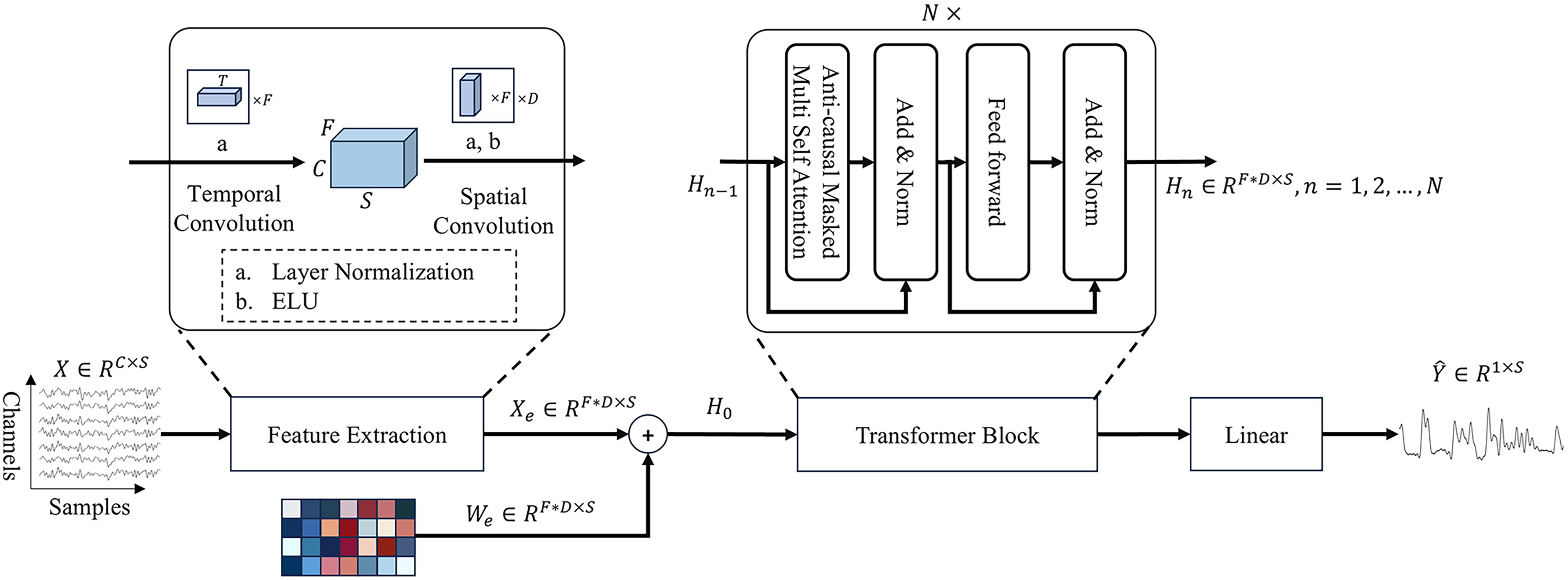
The structure of the auditory decoding transformer (ADT) network consists of three parts: feature extraction layer, transformer block, and linear layer.

The processing of an EEG signal segment $X \in R^{C \times S}$ , where C is the number of EEG electrodes (channels) and S is the total number of samples, commences with a spatio-temporal convolutional layer, which serves to extract both temporal and spatial features. This operation can be encapsulated by the equation:

X_{o} = Act (LN (SC (LN (TC (X)))))

where

TC (\cdot)

denotes temporal convolution,

SC (\cdot)

denotes spatial convolution,

LN (\cdot)

denotes layer normalization (Ba et al., 2016),

Act (\cdot)

is the activation function, and

X_{o} \in R^{F * D \times S}

is the output of feature extraction layer, where F is the number of temporal kernels and D is the number of spatial kernels. In our research,

F = 8

and

D = 4

Subsequent to the feature extraction, the features undergo further processing via a multilayer transformer decoder, a specialized variant of the original transformer architecture proposed by Vaswani et al. (2017). This phase includes the execution of the anticausal masked self-attention mechanism on the input features, followed by the decoding of the speech envelope's high-dimensional features through a forward network layer, culminating in the envelope's derivation through a linear transformation:

H_{0} = X_{o} + PE

H_{n} = transformer_block (H_{n - 1}), \forall n = 1, 2, \dots, N

\hat{Y} = Linear (H_{n})

where N is the number of transformer blocks,

H_{n}

denotes the intermediate features,

\hat{Y}

denotes the estimated envelope,

transformer_block (\cdot)

denotes the transformer block with the anticausal masking, and

PE \in R^{F * D \times S}

denotes the positional encoding matrix from Vaswani et al. (2017) given by

{PE}_{(2 i, pos)} = \sin (pos / 10, 000^{2 i / (F * D)})

{PE}_{(2 i + 1, pos)} = \cos (pos / 10, 000^{2 i + 1 / (F * D)})

where pos is the position and i is the dimension.

The core of $transformer_block$ is the self-attention mechanism with anticausal masking. For the input $H_{n}$ , the output is given by the equation:

AMMSA (H_{n}) = Concat ({head}_{1}, \dots, {head}_{m}) W^{o}

{head}_{i} = softmax (\frac{(H_{n} W_{i}^{Q}) {(H_{n} W_{i}^{K})}^{T}}{\sqrt{F * D}} + Mask) (H_{n} W_{i}^{V})

where m is the number of heads of self-attention,

AMMSA (\cdot)

denotes the anticausal masked multihead self-attention,

W_{i}^{Q}, W_{i}^{K}, W_{i}^{V} \in R^{F * D \times F * D}

, and

W^{o} \in R^{n * F * D \times F * D}

. And

Mask \in R^{F * D \times F * D}

is given by

{Mask}_{i j} = {\begin{matrix} 0, i \geq j \\ - \infty, i < j \end{matrix}

The other component of the $transformer_block$ is the feedforward network, which is implemented using two 1D convolutions with a kernel size of 3 and a hidden dimension of 128. The anticausal masked self-attention layer and the feedforward network layer are connected using residual connections and layer normalization.

The network is optimized using a loss function defined as the negative Pearson correlation coefficient:

Loss = - \frac{\sum_{i = 1}^{S} (\hat{Y_{i}} - \bar{\hat{Y}}) (Y_{i} - \bar{Y})}{\sqrt{\sum_{i = 1}^{S} {(\hat{Y_{i}} - \bar{\hat{Y}})}^{2}} \sqrt{\sum_{i = 1}^{S} {(Y_{i} - \bar{Y})}^{2}}}

where Y denotes the real envelope and S denotes the length of segmentation of envelope. This approach underscores the importance of closely mirroring the true envelope, fostering a deepened understanding and enhanced reconstruction of speech signals from EEG signals.

Why Anticausal Masking? To accurately replicate the anticausal dynamics of speech envelope reconstruction from EEG signals, we incorporate an anticausal masking strategy within the self-attention mechanism of the transformer block. This carefully designed masking approach ensures that, during signal processing at any given moment, the model is restricted to using information from concurrent and future data points only, effectively ignoring preceding signal details. This methodology effectively mirrors the inherent causal sequence from audio stimuli to brain responses, as illustrated in Figure 2, forcing the model to emulate physiological processes in reverse by relying solely on subsequent EEG signals for speech signal reconstruction. By adopting this technique, our model achieves improved accuracy in predicting and reconstructing speech envelopes from EEG inputs, aligning closely with the intrinsic logic and physiological principles governing speech information decoding from EEG signals.

Figure 2.

Three different mechanisms of self-attention. (Left) Anticausal masked self-attention means that reconstructing the speech envelope at the current time depends only on the current and subsequent electroencephalogram (EEG) signal, while causal masked self-attention (right) is the opposite. Normal self-attention (middle) receives information within the entire time samples.

Models for Comparison

Linear Model . The linear decoder model facilitates the reconstruction of the speech envelope from EEG signals by applying linear transformations across all channels and defined temporal windows (500 ms). This model is uniquely implemented using a CNN without any activation functions, distinguishing it from conventional approaches. In a departure from typical methodologies, where a distinct linear decoder is tailored for each participant, this study adopts a unified linear decoder architecture. This design choice is made to ensure a fair comparison with other models evaluated in this research (Accou et al., 2023).

FCNN . The second comparative model in our study is the FCNN, as introduced by Thornton et al. (2022). This architecture is characterized by its multilayer perceptron framework, which employs the Tanh nonlinearity for activation, complemented by batch normalization and dropout strategies to enhance generalization and mitigate overfitting. Drawing upon the insights from Accou et al. (2023), we meticulously selected hyperparameters to optimize the model's performance. These include a learning rate set at 10–3, a batch size of 256, weight decay at 10–6, and a dropout rate of 0.35. The model architecture further incorporates two hidden layers equipped with 1110 and 555 nodes, respectively.

CNN . The third model under comparison is a CNN based on the EEGNet architecture, as described by Thornton et al. (2022), following the principles established by Lawhern et al. (2018). This model is architecturally composed of four key convolutional layers: it initiates with a temporal convolution, succeeded by a deep convolution that amalgamates the channels from the temporal layer. This is followed by an additional deep convolution traversing the temporal dimension. Post each deep convolution phase, a sequence of operations is applied to refine the signal processing: batch normalization to stabilize learning, the exponential linear unit for introducing nonlinearities without hindering the flow of gradients, time-averaged pooling to reduce the dimensionality while preserving temporal features, and spatial dropout to prevent overfitting by randomly omitting units during training. Culminating the architecture, the output from the final convolutional layer is flattened, and an aggregation of all samples is achieved through a fully connected layer endowed with linear activation to make the final predictions. The chosen hyperparameters are as follows: a learning rate of 0.001, a dropout rate of 0.5, F1 set at 4 and F2 at 32 to determine the number of filters in the convolutional layers, D at 8 representing the number of spatial filters, and kernel sizes of 2 and 5 for the average pooling operations.

VLAAI . The fourth model in our comparison is the VLAAI network, proposed by Accou et al. (2023). The VLAAI network is distinguished by its assembly of multiple iterative blocks, each composed of a CNN stack, a fully connected layer, and an output context layer for temporal synthesis. The CNN stack is meticulously designed with five layers, deploying 256 filters in the initial three for broad feature capture and 128 filters in the subsequent two for refined processing. This setup is complemented by a fully connected layer with 64 units and an output context layer that integrates temporal data through additional convolutional layers with 32 and 64 filters. Enhanced with layer normalization, LeakyReLU activation, zero padding for consistent time dimensionality, and jump connections to preserve signal integrity, the network culminates in a linear layer that accurately transforms its complex multilayered output into a concise speech envelope, embodying a cutting-edge approach to auditory signal processing.

Happyquokka . The final model in our comparative analysis is the winner of the Auditory EEG Challenge 2023 (https://exporl.github.io/auditory-eeg-challenge-2023/). It harnesses the power of preconvolution techniques alongside a series of stacked transformers to adeptly decode speech envelopes from EEG signals. In tailoring this award-winning approach to our specific research needs, we undertook strategic optimizations and hyperparameter adjustments. Notably, we streamlined the model by eliminating feature injections related to identity, enhancing its focus on the core task of speech envelope decoding. Additionally, we fine-tuned the architecture by setting the number of stacked transformer blocks to 4, optimizing the balance between complexity and performance (Piao et al., 2023).

Experimental Setups

In this study, we implemented the ADT network utilizing TensorFlow 2.8.0 alongside the recreation of all the comparative models previously discussed. The training process for all models was standardized, using the negative Pearson correlation coefficient as the loss function and the Adam optimizer. The optimizer settings included a learning rate of 10–3, with a decay factor of 0.5 applied after a patience interval after 5 epochs without improvement and an early stopping mechanism activated after 10 epochs without improvement. This rigorous training process was conducted on an NVIDIA RTX A6000 GPU.

For evaluating the models’ performance on the SparrKULee and DTU datasets, we employed the Wilcoxon signed-rank test from the scipy package with Benjamini–Hochberg correction from the statsmodels package. This statistical method was chosen to provide a robust comparison of the models’ output. This analytical approach ensures a thorough and scientifically sound assessment of each model's capability to decode speech envelopes from EEG signals, grounding our findings in statistical significance.

Results

Experiment 1: Self Evaluation

This section focuses on optimizing the hyperparameters for the ADT, specifically the embedding dimension. The initial configuration set the embedding dimension to 64, and the ADT network was trained comprehensively. Upon completion of the training phase, an examination of the linear layer's parameters reveals a significant finding: 40 weights register nearly negligible (absolute value less than 0.05), suggesting a more efficient embedding dimension could be 32. To corroborate this inference, a subsequent visualization of the ADT network, now with the embedding dimension set to 32, was conducted. This adjustment resulted in a more concentrated distribution of parameters within the linear layer, confirming the suitability of a 32-dimensional embedding. Figure 3 illustrates the comparative densities of the linear layer's weights across both ADT networks’ configurations, providing a clear visual endorsement of the 32-dimensional embedding as the more optimal choice.

Figure 3.

Visualization of the weights of the linear layer in auditory decoding transformer (ADT) networks with embed dimensions of 64 (up) and 32 (down). The horizontal coordinate indicates the serial number and the vertical coordinate indicates the value of the weights. Points in blue indicate that the absolute value of the weights is less than 0.05.

Following the selection of the embedding dimension, our next step involved identifying the optimal count of transformer blocks for the ADT network. Figure 4 (left) displays a comparative analysis of the ADT network's performance across a range of transformer block quantities, specifically 1, 2, 4, and 8, on the SparrKULee dataset. Based on this evaluation, we concluded that setting the number of transformer blocks to four strikes the best balance between complexity and performance.

Figure 4.

(Left) Auditory decoding transformer (ADT) network's performance with different transformer blocks; (right) ADT network's training process on SparrKULee dataset.

The configuration of the remaining hyperparameters was informed by insights gained from previous experiments: temporal kernels $(F)$ of 8, spatial kernels $(D)$ of 4, a count of 4 attention heads, a feedforward hidden layer dimension of 128, and an integration window set to 250 ms. In particular, the feedforward neural network consists of two 1D convolution layers of convolution kernels of length 3. Figure 4 (right) then presents the performance metrics, specifically the Pearson correlation coefficients, for both training and validation datasets under these specified conditions. This figure illustrates the model's learning dynamics, demonstrating that a well-optimized ADT network has been established.

Experiment 2: Performance Evaluation

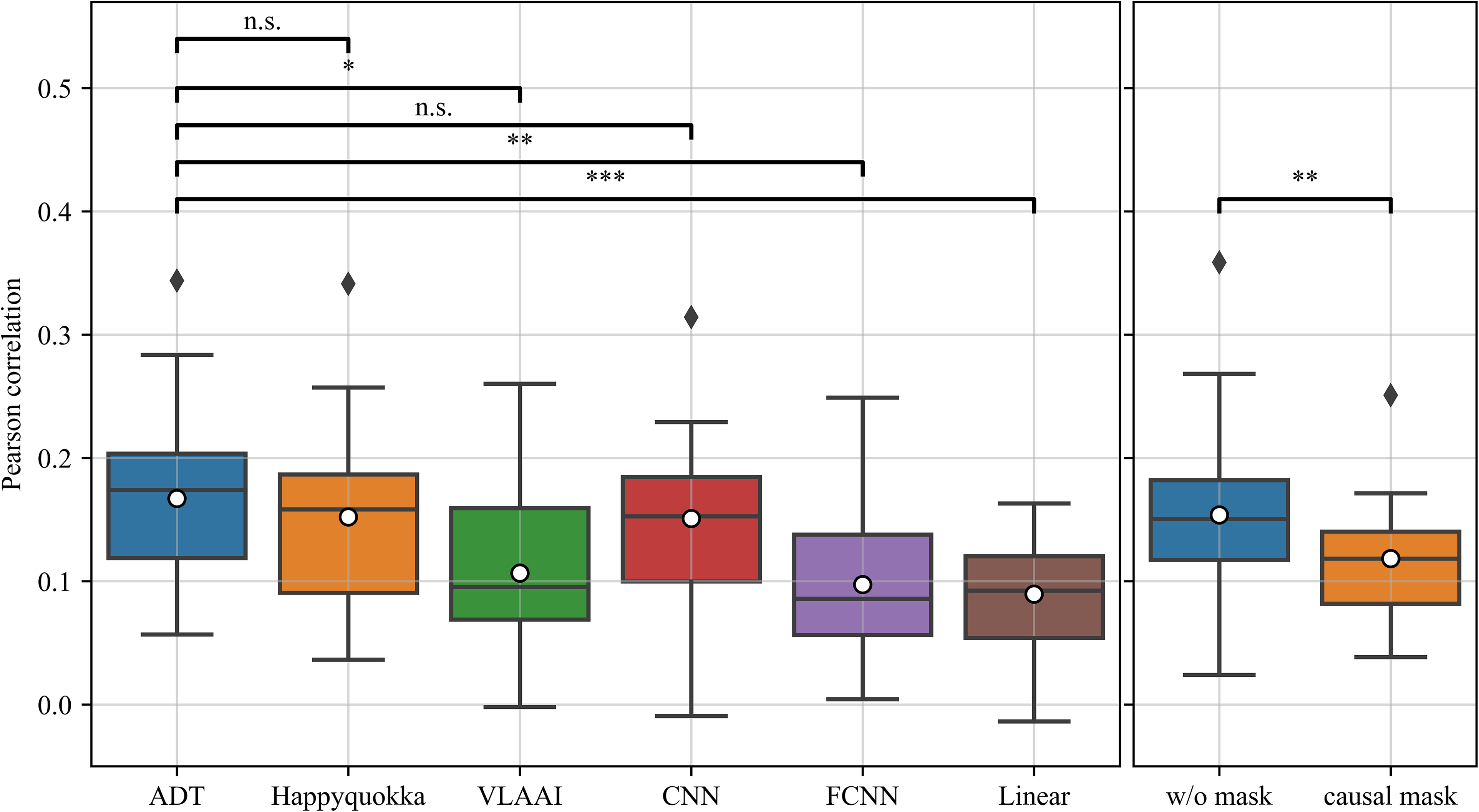
This section presents the performance of ADT on the SparrKULee dataset and the DTU dataset. Figure 5 displays the reconstruction scores of six models in the SparrKULee data. The data points in the figure represent the average reconstruction scores of each subject on the test set. The ADT network has an average reconstruction score of 0.168, which is higher than the average reconstruction scores of 0.159 for Happyquokka (p < .01), 0.130 for VLAAI (p < .001), 0.147 for CNN (p < .001), 0.094 for FCNN (p < .001), and 0.093 for linear model (p < .001). As a complement, we trained the ADT network without masking and using the causal mask with the same conditions. The average reconstruction score of the ADT network without masking is 0.161, which is lower than that of the ADT network with anticausal masking (p < .001) and close to Happyquokka (p > .5). The average reconstruction score for the ADT network with causal masking was 0.146, lower than the ADT network with anticausal masking (p < .001), the ADT network without masking (p < .001), Happyquokka (p < .001), and CNN (p > .05). Theoretically, the ADT network with the causal mask is more suitable as a baseline for envelope reconstruction for nonlinear methods.

Figure 5.

(Left) Comparison of the performance of the auditory decoding transformer (ADT) network and other models on the test set of the SparrKULee dataset. (Right) Comparison of the performance of the ADT network without masking and with causal masking on the test set of the SparrKULee dataset. Each point in the box-and-line plot is a subject's average reconstruction score over all stimuli (n.s.: $p \geq .05$ , *: $.01 \leq p < .05$ , **: $.001 \leq p < .01$ , ***: $p < .001$ ).

Figure 6 displays the reconstruction scores of the six models on the DTU dataset, which was completely invisible to the models during training. The data points in the figure represent the average reconstruction scores for each subject. The average reconstruction score for the ADT network is 0.167, slightly higher than 0.152 for Happyquokka and 0.151 for CNN, but not significantly different. However, it is higher than 0.107 for VLAAI (p < .05), 0.097 for FCNN (p < .01), and 0.090 for linear model (p < .001).

Figure 6.

(Left) Comparison of the performance of the auditory decoding transformer (ADT) network and other models on the DTU dataset. (Right) Comparison of the performance of the ADT network without masking and with causal masking on the DTU dataset. Each point in the box-and-line plot is a subject's average reconstruction score over all stimuli (n.s.: $p \geq .05$ , *: $.01 \leq p < .05$ , **: $.001 \leq p < .01$ , ***: $p < .001$ ).

The average reconstruction score of the ADT network without masking is 0.154, which is slightly lower than that of the ADT network with anticausal masking (p > .05) and close to Happyquokka (p > .5). The average reconstruction score for the ADT network with causal masking was 0.118, lower than the ADT network with anticausal masking (p < .05), the ADT network without masking (p < .01), Happyquokka (p < .05), and CNN (p < .05). Performance evaluation on both datasets demonstrates that the ADT network's ability to reconstruct speech envelopes is comparable to existing state-of-the-art models.

Experiment 3: Interpretability Analysis

In this section, we delve into the interpretability of the ADT network by visualizing its feature extraction layer. This is the advantage of ADT network over other deep learning models. Drawing inspiration from analogous research, our objective is to shed light on the internal mechanics of the ADT network, particularly the construction of the feature representation. Figure 7 showcases the visualization of parameters within the spatio-temporal convolution network layer of the ADT network. This analysis treats the temporal convolution kernels as filters that capture temporal dynamics, while the spatial convolution kernels are projected onto a brain topography. This projection enables visual discernment of the specific contributions of different frequency bands and brain regions to the task of speech envelope reconstruction. This visualization enhances understanding of the ADT network's functionality and facilitates comparison between artificial neural networks and human knowledge.

Figure 7.

Visualization of feature extraction layer’s weights. Each of the eight columns shows the learned temporal kernel and its corresponding frequency domain representation for the 0.25-s window and the four associated spatial kernels. 24 electrodes associated with the temporal lobe were labeled in the brain topography, including 10 temporal lobe electrodes: “F7,” “F8,” “T7,” “T8,” “P7,” “P8,” “FT7,” “FT8,” “TP7,” “TP8,” and 14 electrodes adjacent to the temporal lobe: “F5,” “F6,” “C5,” “C6,” “P5,” “P6,” “AF7,” “AF8,” “FC5,” “FC6,” “CP5,” “CP6,” “PO7,” and “PO8.”

Figure 7 offers a compelling visual distinction among the temporal kernels within the frequency domain. Notably, kernels 4 and 7 demonstrate a pronounced concentration of power within the beta frequency band, signifying their specialized role in extracting information pertinent to this segment of the EEG signal. Moreover, the spatial kernels reveal a pronounced intensity within the temporal lobe region (e.g., spat. kernel 1, temp. kernel 1; spat. kernel 1, temp. kernel 2; spat. kernel 1, temp. kernel 7), a critical area known for processing auditory stimuli and encompassing the auditory cortex. The visualization underscores a darker hue in this region, which aligns seamlessly with clinical insights regarding the auditory cortex's pivotal role in sound perception (Hickok & Poeppel, 2007). Furthermore, some of the spatial kernels display an apparent left–right symmetric distribution (e.g., spat. kernel 2, temp. kernel 6; spat. kernel 3, temp. kernel 8), a pattern that closely mirrors findings from previous studies on reconstructing speech features from EEG signals (Gillis et al., 2022; Van Canneyt et al., 2021; Weissbart et al., 2020). This symmetry reinforces the ADT network's processing fidelity in relation to established neuroscientific observations and highlights its ability to accurately capture and utilize bilateral auditory processing pathways in the brain.

Some spatial kernels show strong activity in the prefrontal lobes (e.g., spat. kernel 2, temp. kernel 3; spat. kernel 3, temp. kernel 2). When combined with the energy distributions in their corresponding temporal kernels, these brain topographies resemble those used to extract eye movements. This is because when independent component analysis (ICA) is used to remove artifacts, similar components to the eye components are usually removed. Previous studies have similarly considered the ability of deep learning models to actively remove noise (Bertoni et al., 2021; Liu et al., 2024).

Following the visualization and analysis phase, we embarked on a further investigation by selectively removing the eight temporal kernels to discern their individual and collective impact on the model's overall performance. To facilitate this, we categorized the temporal kernels into three groups based on their predominant frequency domain characteristics, aiming to unveil the distinct contributions of each frequency band to the speech envelope reconstruction process. These categorizations are as follows: temporal kernels 1, 3, and 6 are associated with low-frequency bands (0.5–8 Hz), serving as indicators of slower neural oscillations; temporal kernels 2, 5, and 8 correspond to mid-frequency bands (8–14 Hz), capturing intermediate neural dynamics; and finally, temporal kernels 4 and 7 are linked to high-frequency bands (14−32 Hz), reflective of rapid neural activities.

To quantitatively assess the influence of these categorically differentiated kernels, we conducted combinatorial ablation studies. In this experimental setup, each kernel or group of kernels was systematically nullified within the model to observe the resultant effect on reconstruction scores. Table 1 presents the outcomes of these ablation studies, showcasing the reconstruction scores on the SparrKULee test set following the strategic zeroing out of specific temporal kernels.

Table 1.

Reconstruction Scores When Temporal Kernel(s) Was/Were Removed in the Test Set of the SparrKULee Dataset.

Kernel(s) removed	Average	SD (±)	Difference
1	0.1035	0.0426	0.0645
2	0.1041	0.0378	0.0638
3	0.1078	0.0433	0.0602
4	0.1018	0.0464	0.0662
5	0.0957	0.0436	0 . 0723
6	0.1013	0.0441	0.0667
7	0.0818	0.0338	0.0862
8	0.1041	0.0430	0.0639
4, 7	0.0683	0.0337	0.0997
1, 3, 6	0.0696	0.0343	0.0983
2, 5, 8	0.0842	0.0323	0.0838
None	0.1680	0.0590	0.0000

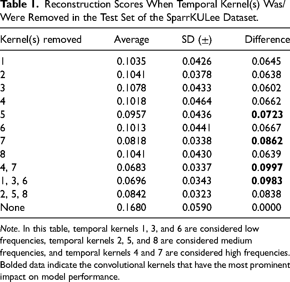
Note. In this table, temporal kernels 1, 3, and 6 are considered low frequencies, temporal kernels 2, 5, and 8 are considered medium frequencies, and temporal kernels 4 and 7 are considered high frequencies.

Bolded data indicate the convolutional kernels that have the most prominent impact on model performance.

In the ablation study, we noted a pronounced impact on the ADT network's performance, particularly when temporal kernels 5 and 7 were subjected to ablation, more so than with the other temporal kernels. Moreover, the removal of temporal kernels associated with high-frequency bands (4 and 7) markedly influenced the ADT's functionality. This observation brings an interesting perspective to the discourse initiated by Thornton et al. (2022) regarding the presumed negligible impact of high-frequency bands on speech envelope reconstruction. Our designation of high-frequency bands within the temporal kernels is predicated on the prominence of their peak frequencies within the frequency domain. Nonetheless, this classification does not imply an exclusive concentration of their energy within the high-frequency spectrum. Notably, temporal kernel 4 retains a portion of its energy within the mid and low-frequency bands, suggesting a potential role in providing auxiliary energy for the reconstruction process.

Finally, we performed a detailed visual analysis of the attention scores. Figure 8 shows the average attention scores in the test set of the SparrKULee dataset. Particularly in the first layer, head 1 and head 4 demonstrate a diagonal pattern, revealing how the ADT network relies on EEG signals within 0–0.5 s to accurately reconstruct the current speech envelope. The discovery of this diagonal pattern not only demonstrates the network's efficiency in time-series analysis but also echoes similar patterns found in previous studies, where time-aligned features are crucial for decoding speech signals.

Figure 8.

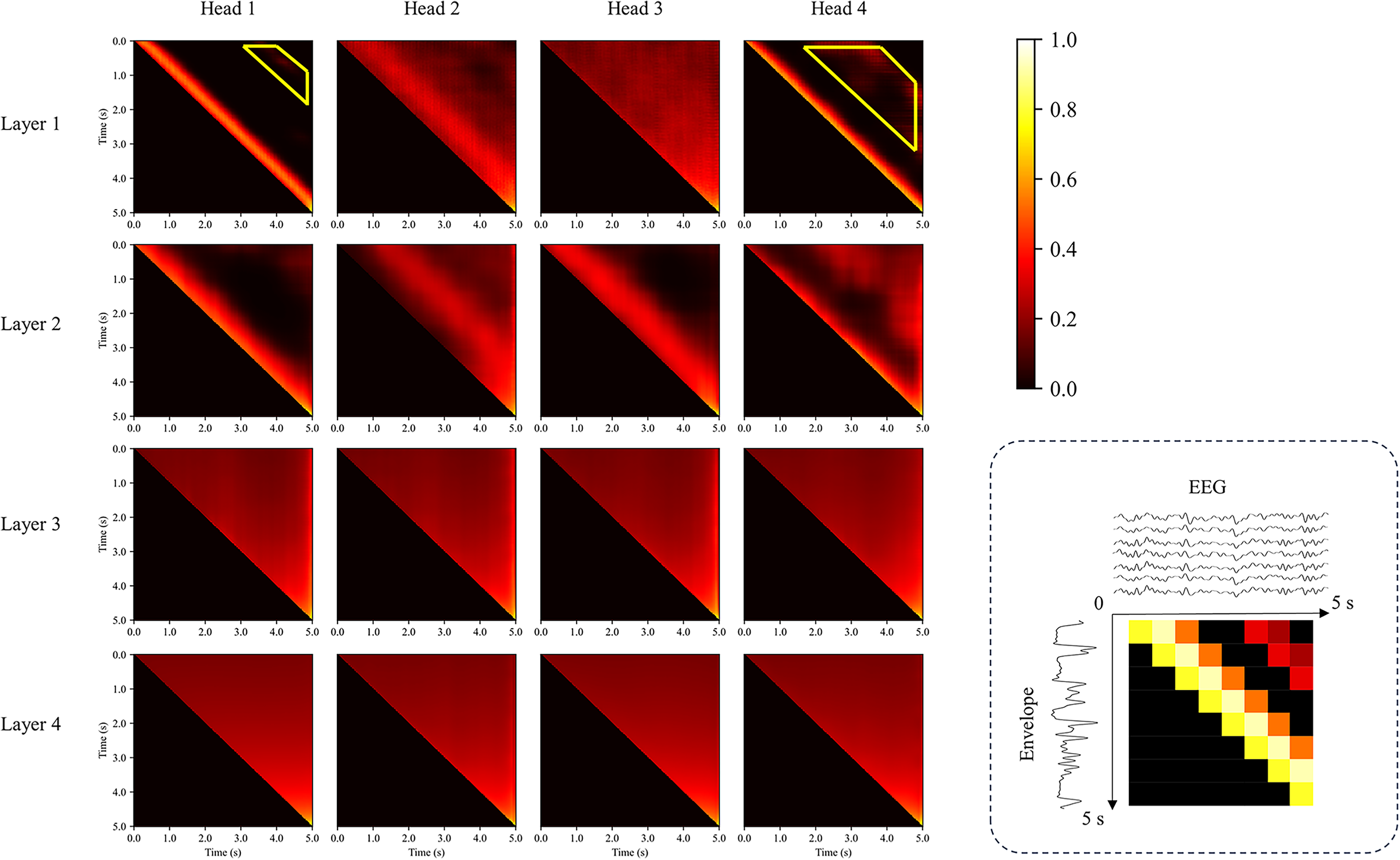
Visualization of attention scores. To enhance image contrast, attention scores are nonlinearly transformed. Attention scores are averaged over a sample of the test set, and they explain the correlation between the envelope and the EEG at different times. The subfigure in the lower right corner is a simple example. Both the horizontal and vertical axes are time axes and are 5 s in length.

Discussion

In this study, we visualized the linear layers within the output layer of the ADT network to determine the embedding dimensions of the model. We also tested the number of transformer blocks to identify the optimal configuration. This parameter adjustment method significantly reduced our workload. Although we did not conduct an exhaustive search of all parameters, the reconstruction performance of the ADT network was comparable to many existing methods used for reconstructing speech envelopes. The ADT network demonstrated impressive performance on the SparrKULee dataset, showcasing its reconstruction capabilities, and also showed generalization capability on the DTU dataset involving cross-linguistic data.

ADT network employs spatio-temporal convolution to extract features from EEG signals, which not only makes the feature extraction process interpretable but also yields compact and informative features. In addition, ADT network introduces the structure of the transformer based on inverse causal masking. Transformer has achieved great success in various time-series tasks by its powerful attention mechanism and parallel processing capability (Wen et al., 2023). By applying transformer to EEG signal decoding, ADT network can better model the long-range dependency between EEG signals and speech envelopes and extract richer and finer speech features.

More importantly, the design of anticausal masking is consistent with the causal relationship of speech signal processing: the brain's response to speech always occurs after the speech signal, but not before it. By using anticausal masking, ADT network can only access the EEG signals of the current and future moments when reconstructing the speech envelope of each moment, but not the past EEG information. This information limitation forces the model to learn more accurate and reliable speech–brain mapping relationships. Experimental results show that anticausal masking significantly improves the envelope reconstruction performance of ADT network compared to variants with no masking or causal masking, confirming the effectiveness of anticausal masking in modeling speech-evoked brain responses. In contrast, other nonlinear models, such as Happyquokka, tend to overlook the speech–brain mapping relationship, which may lead to suboptimal or less stable reconstruction performance. This is evidenced by the observation that Happyquokka's performance is comparable to that of ADT network without masking.

In the medical field, deep learning models often face skepticism due to their lack of interpretability, despite their accuracy and efficiency (Ribeiro et al., 2016). The same challenge exists in deep learning-based speech envelope reconstruction, where the “black box” nature of these networks limits their applicability. Although neural networks like VLAAI have been able to stably reconstruct speech envelopes from EEG signals, mTRF remains the most widely used method (Gonzalez et al., 2024).

To improve the interpretability of the model, we visualized the spatio-temporal convolutional layer parameters and attention scores, revealing the inner workings of the ADT network. This approach aligns with previous research and provides insights that are difficult to obtain in nonlinear models. However, our interpretations of the ADT network, particularly those involving spatial kernels, remain somewhat subjective. Fully quantifying the interpretability of the ADT network and comparing it with traditional linear methods remain a challenge.

We also encountered some issues in interpreting the ADT network. For instance, the yellow trapezoidal region marked in Figure 8 indicates that EEG signals 2–4 s after an event still respond to the current speech, which is significantly more noticeable than in adjacent regions. The reason for this phenomenon remains unclear. This might suggest that nonlinear methods have a potential advantage in capturing long-distance information, which linear methods typically cannot.

Future research should focus on several areas: first, more comprehensive optimization of the model's parameters to further enhance its performance; second, the development of better visualization and interpretation tools to improve model interpretability; and third, validating the model on larger and more diverse datasets to ensure its generalization capability and practical applicability. With these efforts, we believe that the application prospects of the ADT network in the field of speech envelope reconstruction will be further broadened.

Conclusion

This study introduces the ADT network, which utilizes anticausal masking to effectively reconstruct speech envelopes from EEG signals. The ADT network generates embedded features through spatiotemporal convolutions and decodes the speech envelope using stacked anticausal masking transformers. The ADT network achieves performance comparable to state-of-the-art methods while offering interpretability through the visualization of spatiotemporal convolutional layer parameters. It provides new insights into how EEG models can better capture and explain features in recorded EEG responses. The code for the ADT network is made public to maximize its usefulness. The code for this study can be found at https://github.com/ruix6/ADT_Network.

Supplemental Material

sj-docx-1-tia-10.1177_23312165241282872 - Supplemental material for ADT Network: A Novel Nonlinear Method for Decoding Speech Envelopes From EEG Signals

Supplemental material, sj-docx-1-tia-10.1177_23312165241282872 for ADT Network: A Novel Nonlinear Method for Decoding Speech Envelopes From EEG Signals by Ruixiang Liu, Chang Liu, Dan Cui, Huan Zhang, Xinmeng Xu, Yuxin Duan, Yihu Chao, Xianzheng Sha, Limin Sun, Xiulan Ma, Shuo Li and Shijie Chang in Trends in Hearing

Footnotes

Declaration of Conflicting Interests

The authors declared no potential conflicts of interest with respect to the research, authorship, and/or publication of this article.

Funding

The authors disclosed receipt of the following financial support for the research, authorship, and/or publication of this article: This work was supported by the National Key Research and Development Program of China, Natural Science Foundation of Liaoning Province, General Research Program of Liaoning Provincial Department of Education (Grant Nos. 2022YFF1202800, 2021-YGJC14, and JYTMS20230133).

ORCID iD

Shijie Chang

Supplemental Material

Supplemental material for this paper is available online.

References

Accou

Jalilpour Monesi

Van Hamme

Francart

(2021). Predicting speech intelligibility from EEG in a non-linear classification paradigm. Journal of Neural Engineering, 18(6), 066008. https://doi.org/10.1088/1741-2552/ac33e9

Accou

Vanthornhout

Hamme

H. V.

Francart

(2023). Decoding of the speech envelope from EEG using the VLAAI deep neural network. Scientific Reports, 13(1), 812. https://doi.org/10.1038/s41598-022-27332-2

J. L.

Kiros

J. R.

Hinton

G. E.

(2016). Layer normalization. arXiv:1607.06450. http://arxiv.org/abs/1607.06450

Bertoni

Montobbio

Sarti

Citti

(2021). Emergence of lie symmetries in functional architectures learned by CNNs. Frontiers in Computational Neuroscience, 15, 694505. https://doi.org/10.3389/fncom.2021.694505

Bialas

Dou

Lalor

E. C.

(2023). mTRFpy: A Python package for temporal response function analysis. Journal of Open Source Software, 8(89), 5657. https://doi.org/10.21105/joss.05657

Bidelman

G. M.

Price

C. N.

Mahmud

M. S.

Yeasin

(2020). Decoding hearing loss from brain signals. The Hearing Journal, 73(11), 42,44,45. https://doi.org/10.1097/01.HJ.0000722524.69484.01

Bollens

Accou

Van Hamme

Francart

(2023). SparrKULee: A speech-evoked auditory response repository of the KU Leuven , containing EEG of 85 participants. KU Leuven RDR.

Brodbeck

Hong

L. E.

Simon

J. Z.

(2018). Rapid transformation from auditory to linguistic representations of continuous speech. Current Biology, 28(24), 3976–3983.e5.e5. https://doi.org/10.1016/j.cub.2018.10.042

Broderick

M. P.

Anderson

A. J.

Di Liberto

G. M.

Crosse

M. J.

Lalor

E. C.

(2018). Electrophysiological correlates of semantic dissimilarity reflect the comprehension of natural, narrative speech. Current Biology, 28(5), 803–809.e3. https://doi.org/10.1016/j.cub.2018.01.080

10.

Ciccarelli

Nolan

Perricone

Calamia

P. T.

Haro

O’Sullivan

Mesgarani

Quatieri

T. F.

Smalt

C. J.

(2019). Comparison of two-talker attention decoding from EEG with nonlinear neural networks and linear methods. Scientific Reports, 9(1), 11538. https://doi.org/10.1038/s41598-019-47795-0

11.

Crosse

M. J.

Di Liberto

G. M.

Bednar

Lalor

E. C.

(2016). The Multivariate Temporal Response Function (mTRF) toolbox: A MATLAB toolbox for relating neural signals to continuous stimuli. Frontiers in Human Neuroscience, 10, 604. https://doi.org/10.3389/fnhum.2016.00604

12.

Daly

(2023). Neural decoding of music from the EEG. Scientific Reports, 13(1), 624. https://doi.org/10.1038/s41598-022-27361-x

13.

De Cheveigné

Wong

D. D. E.

Di Liberto

G. M.

Hjortkjær

Slaney

Lalor

(2018). Decoding the auditory brain with canonical component analysis. NeuroImage, 172, 206–216. https://doi.org/10.1016/j.neuroimage.2018.01.033

14.

De Clercq

Vanthornhout

Vandermosten

Francart

(2023). Beyond linear neural envelope tracking: A mutual information approach. Journal of Neural Engineering, 20(2), 026007. https://doi.org/10.1088/1741-2552/acbe1d

15.

Ding

Simon

J. Z.

(2012a). Emergence of neural encoding of auditory objects while listening to competing speakers. Proceedings of the National Academy of Sciences, 109(29), 11854–11859. https://doi.org/10.1073/pnas.1205381109

16.

Ding

Simon

J. Z.

(2012b). Neural coding of continuous speech in auditory cortex during monaural and dichotic listening. Journal of Neurophysiology, 107(1), 78–89. https://doi.org/10.1152/jn.00297.2011

17.

Fuglsang

S. A.

Wong

D. D. E.

Hjortkjær

(2018). EEG and audio dataset for auditory attention decoding. Version 1. Zenodo.

18.

Gillis

Decruy

Vanthornhout

Francart

(2022). Hearing loss is associated with delayed neural responses to continuous speech. European Journal of Neuroscience, 55(6), 1671–1690. https://doi.org/10.1111/ejn.15644

19.

Gonzalez

J. E.

Nieto

Brusco

Gravano

Kamienkowski

J. E.

(2024). Speech-induced suppression during natural dialogues. Communications Biology, 7(1), 291. https://doi.org/10.1038/s42003-024-05945-9

20.

Hickok

Poeppel

(2007). The cortical organization of speech processing. Nature Reviews. Neuroscience, 8(5), 393–402. https://doi.org/10.1038/nrn2113

21.

Krishna

Han

Tran

Carnahan

Tewfik

A. H.

(2020). State-of-the-art speech recognition using EEG and towards decoding of speech spectrum from EEG. arXiv:1908.05743. http://arxiv.org/abs/1908.05743

22.

Lawhern

V. J.

Solon

A. J.

Waytowich

N. R.

Gordon

S. M.

Hung

C. P.

Lance

B. J.

(2018). EEGNet: A compact convolutional neural network for EEG-based brain–computer interfaces. Journal of Neural Engineering, 15(5), 056013. Article 5. https://doi.org/10.1088/1741-2552/aace8c

23.

Liu

Chao

Sha

Sun

Chang

(2024). ERTNet: An interpretable transformer-based framework for EEG emotion recognition. Frontiers in Neuroscience, 18, 1320645. https://doi.org/10.3389/fnins.2024.1320645

24.

O’Sullivan

J. A.

Power

A. J.

Mesgarani

Rajaram

Foxe

J. J.

Shinn-Cunningham

B. G.

Slaney

Shamma

S. A.

Lalor

E. C.

(2015). Attentional selection in a cocktail party environment can be decoded from single-trial EEG. Cerebral Cortex, 25(7), 1697–1706. https://doi.org/10.1093/cercor/bht355

25.

Petrosyan

Voskoboynikov

Ossadtchi

(2021). Compact and interpretable architecture for speech decoding from stereotactic EEG. In 2021 Third International Conference Neurotechnologies and Neurointerfaces (CNN) (pp. 79–82). https://doi.org/10.1109/CNN53494.2021.9580381

26.

Piao

Kim

Yoon

Kang

H.-G.

(2023). HappyQuokka system for ICASSP 2023 Auditory EEG challenge. arXiv:2305.06806. http://arxiv.org/abs/2305.06806

27.

Ramirez-Aristizabal

A. G.

Kello

(2022). EEG2Mel: Reconstructing sound from brain responses to music. arXiv:2207.13845. http://arxiv.org/abs/2207.13845

28.

Ribeiro

M. T.

Singh

Guestrin

(2016). Why should I trust you?”: Explaining the predictions of any classifier. Proceedings of the 22nd ACM SIGKDD international conference on knowledge discovery and data mining (pp. 1135–1144).

29.

Thornton

Mandic

Reichenbach

(2022). Robust decoding of the speech envelope from EEG recordings through deep neural networks. Journal of Neural Engineering, 19(4), 046007. https://doi.org/10.1088/1741-2552/ac7976

30.

Van Canneyt

Wouters

Francart

(2021). Neural tracking of the fundamental frequency of the voice: The effect of voice characteristics. European Journal of Neuroscience, 53(11), 3640–3653. https://doi.org/10.1111/ejn.15229

31.

Vaswani

Shazeer

Parmar

Uszkoreit

Jones

Gomez

A. N.

Kaiser

Polosukhin

(2017). Attention is all you need .

32.

Wang

Chen

Khalilian-Gourtani

Chen

Flinker

Wang

(2020). Stimulus speech decoding from human Cortex with generative adversarial network transfer learning. 2020 IEEE 17th international symposium on biomedical imaging (ISBI) (pp. 390–394).

33.

Weissbart

Kandylaki

K. D.

Reichenbach

(2020). Cortical tracking of surprisal during continuous speech comprehension. Journal of Cognitive Neuroscience, 32(1), 155–166. https://doi.org/10.1162/jocn_a_01467

34.

Wen

Zhou

Zhang

Chen

Yan

Sun

(2023). Transformers in time series: A survey. arXiv:2202.07125. http://arxiv.org/abs/2202.07125

35.

Wong

D. D. E.

Fuglsang

S. A.

Hjortkjær

Ceolini

Slaney

De Cheveigné

(2018). A comparison of regularization methods in forward and backward models for auditory attention decoding. Frontiers in Neuroscience, 12, 531. https://doi.org/10.3389/fnins.2018.00531

36.

Zhou

Unoki

Zhang

Dang

(2022). Reconstruction of speech spectrogram based on non-invasive EEG signal. 2022 13th international symposium on chinese spoken language processing (ISCSLP) (pp. 275–279).

Supplementary Material

Please find the following supplemental material available below.

For Open Access articles published under a Creative Commons License, all supplemental material carries the same license as the article it is associated with.

For non-Open Access articles published, all supplemental material carries a non-exclusive license, and permission requests for re-use of supplemental material or any part of supplemental material shall be sent directly to the copyright owner as specified in the copyright notice associated with the article.

0.00 MB

2.21 MB