
Abstract
Most human auditory psychophysics research has historically been conducted in carefully controlled environments with calibrated audio equipment, and over potentially hours of repetitive testing with expert listeners. Here, we operationally define such conditions as having high ‘auditory hygiene’. From this perspective, conducting auditory psychophysical paradigms online presents a serious challenge, in that results may hinge on absolute sound presentation level, reliably estimated perceptual thresholds, low and controlled background noise levels, and sustained motivation and attention. We introduce a set of procedures that address these challenges and facilitate auditory hygiene for online auditory psychophysics. First, we establish a simple means of setting sound presentation levels. Across a set of four level-setting conditions conducted in person, we demonstrate the stability and robustness of this level setting procedure in open air and controlled settings. Second, we test participants’ tone-in-noise thresholds using widely adopted online experiment platforms and demonstrate that reliable threshold estimates can be derived online in approximately one minute of testing. Third, using these level and threshold setting procedures to establish participant-specific stimulus conditions, we show that an online implementation of the classic probe-signal paradigm can be used to demonstrate frequency-selective attention on an individual-participant basis, using a third of the trials used in recent in-lab experiments. Finally, we show how threshold and attentional measures relate to well-validated assays of online participants’ in-task motivation, fatigue, and confidence. This demonstrates the promise of online auditory psychophysics for addressing new auditory perception and neuroscience questions quickly, efficiently, and with more diverse samples. Code for the tests is publicly available through Pavlovia and Gorilla.
Introduction
Much of what we know about the function of the auditory system is due to a century of auditory psychophysical behavioral paradigms in human listeners. Auditory psychophysics tends to rely on strongly sound-attenuated environments, finely calibrated equipment, and small numbers of expert or highly trained listeners who are motivated and compliant with task demands. This high level of what we term ‘auditory hygiene’ is important: seemingly minute differences in stimulus delivery and timing, background noise levels, or participant engagement during attention-demanding paradigms for measuring perceptual thresholds can dramatically affect experimental results (Green, 1995; Manning et al., 2018; Rinderknecht et al., 2018).
The COVID pandemic taught us the utility of online testing and challenged how we maintain auditory hygiene when lab facilities are inaccessible; the need to include more diverse and representative participant samples has also driven a move toward more inclusive experimental environments (Henrich et al., 2010; Rad et al., 2018) particularly using online experimentation services (Anwyl-Irvine et al., 2020; Buhrmester et al., 2011; Peirce et al., 2019, p. 2; Sauter et al., 2020). As highlighted in a recent report by the ASA Task Force on Remote Testing (https://tcppasa.org/remote-testing/) human auditory researchers have created a number of methods to maintain high standards using out-of-laboratory testing. For instance, several groups have created tests for ensuring participants are using headphones rather than speakers (Milne et al., 2020; Woods et al., 2017), and that they are engaging with the experimental task, rather than haphazardly pressing buttons (Bianco et al., 2021; Mok et al., 2021; Zhao et al., 2019). Such innovations notwithstanding, uncontrolled online experimental situations are particularly challenging for auditory paradigms that deliver stimuli within a range of sound pressure levels, or that require sustained vigilance to respond consistently to an ever more difficult-to-perceive target sound.
Control of the range of sound pressure levels is important for ensuring participants’ well-being, making sure they are not exposing themselves to overly loud sounds. Sound pressure level is also important because neuronal responses from the cochlea to cortex are known to differ as a function of overall level. For instance, subpopulations of auditory nerve fibers differing in spontaneous firing rates respond at different acoustic stimulation levels (Horst et al., 2018; Taberner & Liberman, 2005). Across the peripheral and central auditory systems, single neuronal responses tend to be level-dependent, with frequency selectivity typically broadening with increasing sound amplitude levels (Bizley et al., 2005; Schreiner et al., 2000). Behaviorally derived auditory filter widths have also been shown to be level-dependent (Glasberg & Moore, 2000; Pick, 1980). This is particularly important for experiments that aim to compare perceptual versus attentional auditory filters, such as in the classic 'probe-signal' paradigm presented below (Anandan et al., 2021; Borra et al., 2013; Botte, 1995; Dai & Buus, 1991; Dai et al., 1991; Green & McKeown, 2001; Greenberg & Larkin, 1968; Macmillan & Schwartz, 1975; Moore et al., 1996; Scharf et al., 1987; Scharf et al., 1987; Tan et al., 2008).
Many auditory experiments, including the probe-signal paradigm, typically ask listeners to perceive stimuli at or near their perceptual thresholds for hearing out a stimulus in quiet or in a masking noise or background. These thresholds can differ considerably across individuals, so often experimental sessions will begin by running adaptive psychophysical paradigms to estimate the individual's relevant perceptual thresholds. Obtaining reliable auditory psychophysical thresholds can be challenging, even in laboratory conditions with experienced and motivated adult listeners. For example, thresholds-in-quiet have been shown to be affected by the duration of time spent in a ‘quiet’ environment (Bryan et al., 1965; Steed & Martin, 1973) such as an audiometric booth. Even supra-threshold detection tasks performed by experienced listeners can be affected by presentation level (Williams et al., 1978). Determining reliable psychoacoustical thresholds may be especially hard with inexperienced listeners (Kopiez & Platz, 2009) or in the presence of distracting events (Ruggles et al., 2011) typical of a home environment.
Especially for online studies where participants are in their home environments, reduced levels of engagement and vigilance due to listeners’ motivation, fatigue, and confidence can inject additional noise and bias (general discussion in Elfadaly et al., 2020). This is particularly true when paradigms required to set perceptual levels for the actual experiments of interest are themselves potentially tedious and unrewarding (reviewed in Jones, 2019). Multiple long thresholding tracks also add considerable expense to online experiments, which tend to rely on shorter experimental sessions with larger numbers of participants to compensate for participant variability. A number of investigators have optimized psychophysics techniques for measuring perceptual thresholds in different populations. For instance, Dillon et al. (Dillon et al., 2016) used Monte Carlo simulations to create an efficient adaptive algorithm for telephone-based speech-in-noise threshold measurement. Others have designed 'participant-friendly' procedures for pediatric psychoacoustics testing (for example, Halliday et al., 2017) that manipulate different stepping rules, for instance changing reversal rules once a first error has been made (Baker & Rosen, 2001).
Nonetheless, lapses in attentive listening in repetitive and challenging tasks like the staircase threshold setting procedures described above can dramatically impact experimental results. Thus, concern that anonymous, online participants may be less motivated to perform to the best of their abilities, as compared to more traditional in-person expert listeners has contributed to reticence in moving auditory investigation online.
In a set of three experiments, we address the challenges of sound level setting, psychophysical threshold estimation, and participant motivation, engagement and vigilance in online auditory psychophysics experiments. To this end, we test new online versions of level setting and threshold-in-noise paradigms, as well as a short-duration online version of the aforementioned probe-signal paradigm. We also evaluate whether results are potentially modulated by participants’ motivation and fatigue levels.
In Experiment 1, we assess a method for controlling the range of experimental stimulus levels (within ± 10 dBA SPL) in online testing conducted in uncontrolled environments. To do this, we have participants act as a 'self-calibrated audiometer' by listening to a white or pink noise stimulus with a particular root-mean-square amplitude (RMS), then adjusting the volume setting on their own computer to a just-detectable threshold. 1 To assess the validity of this approach, participants take part in the online amplitude setting task in uncontrolled environments and in the laboratory.
In Experiment 2, we incorporate the level-setting paradigm introduced in Experiment 1, then ask whether small adjustments to standard thresholding procedures for a classic psychophysical task (tone detection in white noise) will permit fast (2–3 min) and reliable estimation of thresholds among participants recruited and tested online. Specifically, we evaluate three factors. One, we test the reliability of estimates over three short (40-trial) staircase-based thresholding tracks. Two, we examine whether a simple estimator of psychophysical threshold - the statistical mode of levels across a thresholding track (e.g., the most frequently visited level) - is as robust or more robust at estimating threshold as traditional estimators based on staircase reversals. Three, we determine whether and how online psychophysical thresholds are related to established assays of participant fatigue, apathy, and task confidence.
In Experiment 3, we use the online tone-in-noise thresholding procedure from Experiment 2 to set participants thresholds for a new online version of the probe-signal paradigm (Botte, 1995; Dai & Buus, 1991; Dai et al., 1991; Greenberg & Larkin, 1968; Moore et al., 1996; Scharf et al., 1987). After completing the online threshold-setting procedure of Experiment 2, the same online participants heard continuous noise in which an above-threshold tone was followed by two listening intervals. Participants reported the interval in which a near-threshold tone was embedded in the noise, with the tone frequency matching the cue on 75% of trials and mismatching the cue at one of four other frequencies on 25% of the trials. We sought to determine whether patterns of frequency-selective attention: 1) can be replicated in uncontrolled online testing environments with naive listeners; 2) are evident in the short testing sessions necessitated by online testing; 3) change and develop over testing trials; and 4) are related to established assays of participant fatigue, apathy, and task confidence.
We provide code for each of these approaches to facilitate improved ‘auditory hygiene’ in online experiments, and to demonstrate the possibilities for asking new questions in auditory science with classic, yet challenging, online psychophysical paradigms. Our goal is to test and validate procedures for good 'auditory hygiene' in less controlled environments so that online studies can be as rigorous as (and directly compared to) in-lab studies.
Experiment 1
In the four conditions of Experiment (Expt) 1a-d (see Table 1), we ask whether we can control the range of experimental stimulus levels in online testing conducted in different environments. Our approach involves playing a reference white or pink noise segment and having young adult online participants with healthy hearing adjust the volume setting on the computer to just-detectable levels. Rather like the “biological check” employed daily to confirm (though not adjust) level calibration in most audiology clinics, this procedure allows for each participant to use their normal hearing thresholds to adjust for their unique testing equipment and acoustic environment. The RMS amplitude of the white noise stimulus used for setting this detection threshold is then used as a reference value for setting the amplitude of subsequent experimental stimuli during the same session.
Overview of Experiment 1. Details Differentiating Experiments 1a-d are Shown.
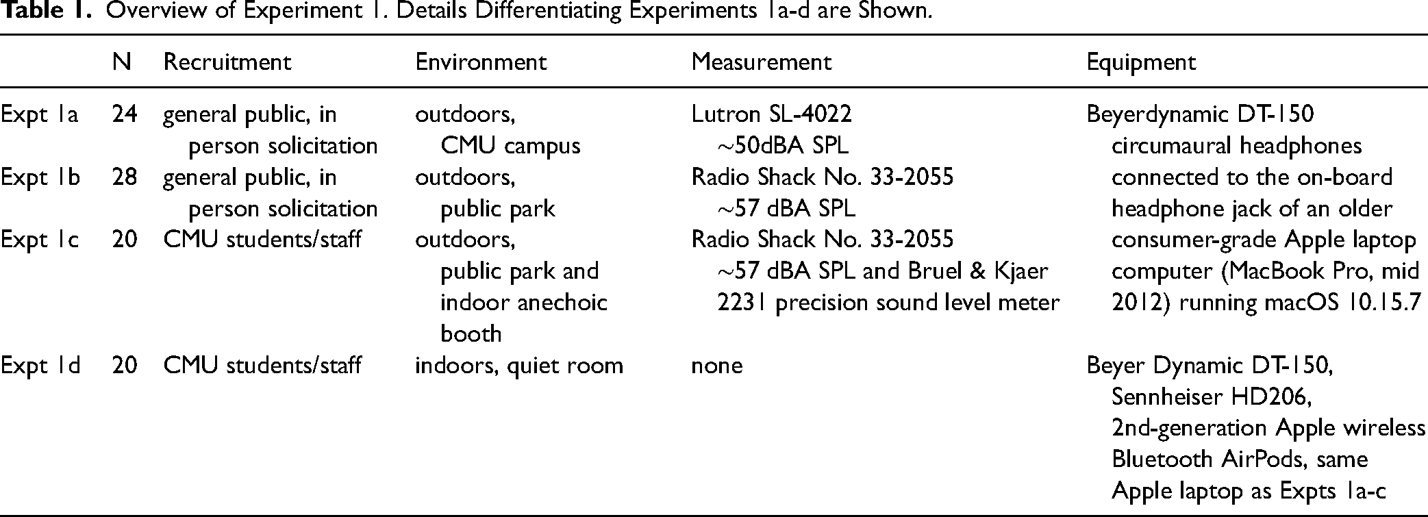
In Expt conditions 1a and 1b, we tested different members of the general public outdoors using a pulsed bandpass-filtered white noise; given the level of distraction and background sound, these experiments provide initial real-world tests of the level setting paradigm. In condition 1c, we tested a group of Carnegie Mellon University affiliates to assess the reliability of the level setting paradigm over different listening conditions by having the same participants complete the task outdoors and in an anechoic chamber. Finally, in condition 1d, we tested another group of Carnegie Mellon University affiliates with bandpass-filtered white and pink noise to ask how level setting might be affected by spectral shape; to assess consistency across headphones, the same participants were also tested with white noise only using two different headphones as well as a popular brand of earbuds.
Methods
Participants
Validation of the online level setting procedure required testing in-person participants on a common consumer laptop with consumer headphones (with headphone type manipulated across conditions). For Expts 1a and 1b, recruitment was primarily conducted via informal in-person solicitation in outdoor environments due to COVID-related restrictions on indoor activities that were in place during data collection, and because the total task duration was approximately 2 min. For Expt 1a, participants (N = 24) were recruited in an open lawn on the Carnegie Mellon University campus; a subset of participants were graduate students at a departmental gathering, others were undergraduate students as well as parents visiting for graduation ceremonies. Expt 1a participants were asked only whether they were at least 18 years of age, and considered their hearing to be within normal ranges, similar to the information that is solicited in many online studies. For Expt 1b, participants (N = 28) were recruited in a central Pittsburgh park from a more heterogenous pool; here, participants were asked to note their age (mean age = 27.9 years (SD 10.2), ranging between 18 and 55 years). One of these participants mentioned that they occasionally wore hearing aids. For Expt 1c, all participants were Carnegie Mellon or University of Pittsburgh students or staff (N = 20; mean age = 30.1 years (SD 9.2), age range 17–47 years); here the same individuals were tested in the outdoor environment as well as in an anechoic sound booth under well-controlled laboratory conditions. For Expt 1d, all participants were Carnegie Mellon students or staff (N = 20, mean age = 25.4 years (SD 5.2, age range 18–37 years; these were not the same participants as Expt 1c).
The study was approved by the Birkbeck College ethics committee (181941/200518) for online testing without geographic restrictions, and took approximately 2 min to complete, including reading and completing the consent form, reading instructions, and performing the amplitude-setting task. Face-to-face participants were covered by local Carnegie Mellon University or University of Pittsburgh IRB protocols, as appropriate.
Stimuli and Equipment
Using Praat 6.0.17 (Boersma & Weenink, 2021) a 1 s Gaussian white noise was generated, and band-pass filtered between 80–8000 Hz to restrict high-frequency contributions to overall intensity and low-frequency line noise. The RMS amplitude within Praat was adjusted to 0.000399 (26 dB). This amplitude setting was chosen as pilot testing suggested it allowed thresholds-in-quiet to be achieved within the range of laptop volume control settings (see Stimulus Analysis section below for analysis of analog stimulus output from two laptops).
Raised-cosine onset and offset ramps of 100 ms were added, so that when played on a continuous loop without gaps, it would sound like a sequence of pulsed noises. The audio data were stored in the WAV file format, then exported in Sox (http://sox.sourceforge.net/) to a stereo (diotic) sound file in the lossless FLAC format. This RMS level of this stimulus file serves as the amplitude reference for the sound stimuli in Expts 2 and 3. For Expt 1d only, a pink noise stimulus (with 1/f power spectral density) with the same duration, onset/offset ramps, and RMS as the white noise was also saved to FLAC format.
For Expts 1a-c, stimuli were presented using Beyerdynamic DT-150 circumaural headphones connected to the on-board headphone jack of an older consumer-grade Apple laptop computer (MacBook Pro, mid 2012) running macOS 10.15.7. For Expt 1d, which tested the procedure with different grade headphones, the Beyerdynamic DT-150 (∼$200 US), along with Sennheiser HD206 (∼$20 US), and 2nd-generation Apple wireless Bluetooth AirPods (∼$150 US) were used with the same Apple laptop.
For experiments 1a-c, outdoor sound levels were measured using a Lutron SL-4022 (Expt 1a) or a Radio Shack Cat No. 33-2055 sound level meter (Expt 1b and 1c). For Expt 1a, Baseline average sound levels were ∼50 dB SPL A-weighted; for Expt 1b, they were somewhat higher, with an average of ∼57 dBA SPL, ranging between ∼53–67 dBA SPL. For Expt 1c, sound levels were an average of 31 dBA SPL indoors in the anechoic chamber (using a Bruel & Kjaer 2231 precision sound level meter) and 57 dBA SPL outdoors. As with many real-world listening environments, the outdoor environments included frequent sound events of somewhat higher amplitude (bird chirps, conversations of passing people, motorized skateboards, and helicopters flying overhead). See Supplemental Figure S1 for power spectral densities of the acoustic environments used in Expt 1c. (Expt 1d was conducted indoors in quiet rooms so we did not measure ambient sound levels).
Calibration
For each volume setting increment on the MacBook Pro, dB SPL measurements were obtained using a Bruel & Kjaer 2231 precision sound level meter set to slow averaging and A-scale weighting and Bruel & Kjaer 4155 ½” microphone mounted in a Bruel & Kjaer 4152 artificial ear with a flat-plate coupler, coupled to the same set of Beyer DT-150 headphones used for data collection. Stimuli were played with exactly the same procedure and Macbook Pro as used for participant testing. This calibration routine was conducted in an anechoic chamber located on the University of Pittsburgh campus with an ambient noise floor measured to be about 31 dBA SPL using the same Bruel & Kjaer meter and coupler set up, as detailed above, but with the headphones disconnected. Note that the coupler simulates ear canal resonance, which when paired with A-Scale weighting, magnified the associated band-pass filtering and thus likely underestimated SPL at the eardrum.
Because the SPL of the stimulus at the lowest volume settings was below this noise floor, the white noise stimulus was digitally increased in level by 10 and 20 dB, and SPL values were then recorded at all volume settings for these two more intense stimuli, as well as for the original stimulus used during testing. The SPL-Volume setting functions generated using the more intense stimuli were then used to extrapolate the same function from the original stimulus below the noise floor (See Figure 1). Volume setting adjustments were determined to be linear on the MacBook Pro used in the amplitude setting experiment, e.g., a given increment in volume setting generated a relatively consistent change in dBA SPL at both high and low overall levels. This result gave us confidence that we could extrapolate downward to and below the noise floor. For a fuller picture of measuring below the noise floor, please see Ellingson et al. (2015) and Whittle and Evans (1972).
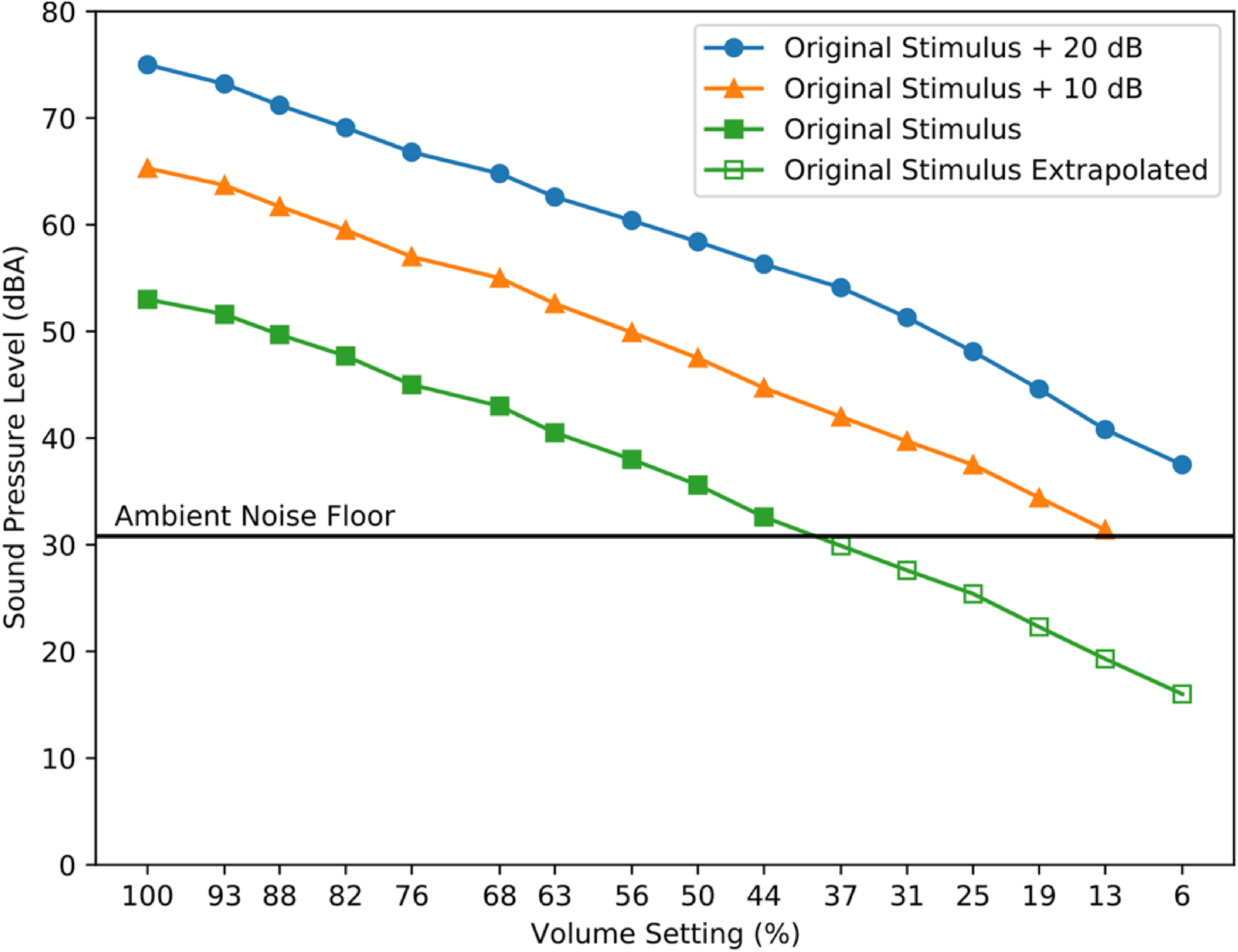
Sound pressure levels of the noise stimulus as a function of computer volume setting percentages. The noise stimulus was the same bandpass-filtered white noise used for testing or was increased in intensity by 10 or 20 dB. Measurements were made by playing each stimulus at each volume setting of the Macbook Pro using the headphones used in Experiments 1a-1c, coupled to an artificial ear. Because the SPL of the stimulus at the RMSv used for testing was below the ambient noise floor at lower volume setting values, the volume-setting functions at + 10 and + 20 dB were used to extrapolate the test stimulus function. SPL is in dBA.
The results of this acoustic analysis indicated that the highest volume setting (100%) produced a stimulus presentation level of 55 dBA SPL, and the lowest (6%) corresponded to 19.3 dBA SPL. Figure 1 shows dBA SPL values for the band-passed white noise stimulus at various levels (original level used during testing, and + 10 and + 20 dB) at each volume setting.
Recording and Analysis of Laptop Stimulus Output to Headphones
In order to deliver sound levels near detection threshold via standard laptops and headphones, the RMS of the white noise audio file needed to be very low (0.000399), raising the possibility that the signal would be distorted due to low bit depth, and would also fall below the noise floor of the sound card. To test this, we recorded the electric headphone jack output of a MacBook Pro as well as an older Asus Windows laptop, and compared the power spectrum of line noise alone to that of the white noise stimulus at the laptop volume settings corresponding to the range of participants’ reported thresholds (See Supplemental Materials and Figure S1 for full details). Power across stimulated frequencies was consistently above noise floor for all volume settings reported as white noise thresholds (from ∼ + 5dB to + ∼14dB for MacBookPro volume setting 18 to 44%), did not change appreciably in spectral shape, and floor noise levels are consistent across volume settings. We also tested the pink noise thresholding stimulus with same RMS as the white noise (used in Expt 1d below); as would be expected, at lower frequencies (< ∼1 kHz) there was a greater difference in power between the pink noise stimulus and noise floor than with the white noise (see Supplemental Materials).
Experimental Procedure
For all experimental conditions, sounds were presented with the Pavlovia.org (Peirce et al., 2019) online experimental platform using Google Chrome version 09.0.4430.212 via wireless connections to various broadband providers. Written instructions presented on the laptop screen asked participants to adjust the computer’s volume setting to about 50% and then to click a button labeled ‘play’ to hear the pulsed noise played on a continuous loop until the participant pressed pause or proceeded to the next page. The continuous loop was achieved by in-house JavaScript code and no gap was inserted between the repetitions. Next, participants were instructed to use the computer’s volume setting buttons on the keyboard to adjust the level of the noise so that it was barely audible. Specific instructions directed participants to slowly lower the volume setting until they could no longer hear the noise, and then to increase the volume setting one increment at a time, until they could again just barely hear the noise. After the participant was satisfied with their setting, the experimenter manually recorded the final volume setting as a percentage of full volume. As with many computers, the Mac volume setting buttons permit only a discrete range of percentage values. The only possible percentage settings were [0 6 12 19 25 31 38 44 50 56 62 69 75 81 88 94 100]. A demonstration of the procedure is available at [https://run.pavlovia.org/sijiazhao/volumechecking_demo]. The implementation is available in JavaScript [https://gitlab.pavlovia.org/sijiazhao/volumechecking_demo] and via the Gorilla experimental platform [https://gorilla.sc/openmaterials/261557].
For Expt 1a and 1b (outdoor experiments), participants only performed the task once. For Expt 1c, participants performed the task once outdoors, and then once in the anechoic chamber. For Expt 1d, participants performed four variants of the paradigm. Wearing the Beyer Dynamic DT-150 headphones, participants set levels using 1) white and 2) pink noise stimuli. They also set levels using the white noise stimulus only while wearing 3) Sennheiser HD206 headphones and 4) Apple AirPods. The order of these four variations was counterbalanced over the 20 participants.
Results
Experiment 1a (Participants Tested Outdoors at Carnegie Mellon University)
Participants set their “just detectable” levels, an estimate of the audibility threshold, by choosing volume settings that were between 19–50%, a range that corresponds to 22.3–35.6 dBA SPL, with a mean dBA SPL setting of 29.43 (standard deviation (SD) 3.95, Figure 2(a)).

Perceptual thresholds set in expt 1a-c. (a) Frequency histogram showing the number of Expt 1a participants who set their perceptual threshold at each volume setting/dBA SPL level, as established in the anechoic calibration procedure. The top row of the x-axis shows estimated dBA SPL level; the bottom row of the x-axis shows the range of the corresponding MacBook Pro volume settings. (b) Frequency histogram showing the number of Expt 1b participants who set their perceptual threshold at each dBA SPL. The top row of the x-axis shows estimated dBA SPL; the bottom row of the x-axis shows the range of the corresponding MacBook Pro volume settings. (c) Scatterplot showing Expt 1c data from the same participants, collected indoors in the anechoic chamber (x-axis), and outdoors in a Pittsburgh park (y-axis). The black line shows best linear fit; individual data points are slightly jittered to show all 20 individuals. (d) Frequency histogram showing the number of Expt 1c participants who set their perceptual threshold at each dBA SPL, for indoor (anechoic chamber) and outdoor (park) settings.
Experiment 1b (Participants Tested Outdoors in Central Pittsburgh Park)
Participants’ white noise perceptual thresholds were somewhat broader than in Expt 1a. Volume settings were between 19 and 76%, a range corresponding to 22.3–45.0 dBA SPL, and a mean dBA SPL of 33.05 (SD 5.62, Figure 2(b)).
Experiment 1c (Participants Tested Both Outdoors and in Psychoacoustic Laboratory Settings)
As with the previous experiments, participants’ white noise detection thresholds were converted from the MacBook Pro percent volume setting to dB SPL using the data and extrapolation shown in Figure 1. Results in both settings replicated the previous experiments, with participants’ indoor volume settings ranging between 19–50% (22.3–35.6 dBA SPL, mean 26.59 dBA SPL, SD 3.83), and outdoor settings ranging between 25–63% (25.4–40.5 dBA SPL, mean 31.24 dBA SPL, SD 4.31).
Figure 2(c) shows that participants’ noise detection thresholds in anechoic and outdoor conditions were highly correlated (Pearson r = 0.82, p < .001, verified using nonparametric Spearman rho = 0.70, p < .001). There was a modest average increase of 4.66 dBA SPL in the threshold values from anechoic to outdoor settings (Figure 2(d)). This mean increase in threshold seems reasonable despite the relatively large difference in ambient noise levels (31 dBA SPL indoors, and 57 dBA SPL outdoors). An inspection of the relative power spectral densities (see Supplementary Materials Figure S2) shows that while there are large differences at low frequencies, those differences are smaller near the upper end of the frequency band of the test stimulus (indicated by the shaded area). It may also be that the outdoor noise sources are relatively localizable, and thus more easily segregated from the stimulus during testing.
Because participant age can interact with both pure-tone hearing thresholds as well as listening in noise, we assessed the potential effects of age on estimated thresholds in outdoor settings by combining data from Expts 1b and 1c (Figure 3(a)). Using a regression analysis including age in years as well as cohort (participants in Expt 1b or Expt 1c), the overall model was significant (ANOVA, F(2,45) = 4.87, p < .0121), with no significant effect of cohort (t = 1.60, p = .12), and a significant moderate effect of age (t = 2.84, p = .0067, slope estimate 0.204). There were two people who had relatively high thresholds (45 dBA SPL); one participant (age 40) mentioned they occasionally wore hearing aids.

Perceptual thresholds in expt 1a-c. (a) Scatterplot showing the relationship between Expt 1b and 1c participant age (on the x-axis) and estimated dBA SPL threshold on the y-axis. The crosses present the individual data from Expt 1b and the gray circles present the individual data from Expt 1c (two experiments N = 48 in total). The thick and thin dashed lines show the best fit between age and dBA SPL threshold when cohort (participants in Expt 1b or 1c) is included in the regression model. (b) Histogram of perceptual thresholds set by participants who were tested outdoors in all Expts 1a-1c (n = 72) is shown, with the black bins indicating the number of participants who set their perceptual threshold at each dBA SPL.
Across Expts 1a-1c (N = 72 total participants tested outdoors, Figure 3(b)), the median noise detection threshold was 29.90 dBA SPL, with the 10th and 90th percentiles at 25.40 and 38 dBA SPL. For very quiet indoor settings, extrapolating from the Expt 1c outdoor versus indoor within-subjects experiment showing a 4.66 dB level difference, we would expect a median detection threshold of 25.95 dBA SPL with 10th and 90th percentiles of 22.30 and 32.75 dBA SPL. The 25.15 dB (14.1 to 39.25 dBA SPL) range of sound detection thresholds is similar to the ∼25dB range of hearing reported for the 5th-95th percentile of normal hearing adults 18–40 years of age (Park et al., 2016); this assumes that assessment of auditory thresholds with different pure tone frequencies and 80 Hz–8000 Hz bandpass-filtered white noise are comparable, an assumption with limited evidence, to our knowledge (Carrat et al., 1975).
Experiment 1d (Participants Tested Using White and Pink Noise, and Different Headphones and Earbuds)
We first compared levels set using white and pink noise while participants wore the Beyer Dynamics D-150 headphones in quiet conditions. Participants’ white noise thresholds ranged between 25–44% volume setting (25.4–32.6 dBA SPL) and were very highly correlated with their pink noise thresholds (Spearman's rho = 0.83, p < .0001, see Figure 4(a)). There was a significant offset, where levels set with pink noise were on average one volume increment higher compared to white noise (Wilcoxon signed-rank, S = 100, p < .0001), corresponding to a ∼2dB difference. Next, we compared white noise thresholds set when using the Beyer Dynamics D-150 versus the Sennheiser HD206 and Apple AirPods. Thresholds set with the Beyer Dynamics D-150 were significantly correlated with those set with the Sennheisers (Spearman's rho = 0.65, p = .0021; Figure 4(b)), and with the AirPods (Spearman's rho = 0.69, p = .0008; Figure 4(c)). Threshold volume settings were on average reliably but just slightly (0.75 volume control increments) higher with the Beyer Dynamics (mean = 33.2%) than with the Sennheisers (mean = 28.5%, Wilcoxon signed-rank, S = 82.5, p < .001). By comparison, threshold volume settings were an average of 3.05 higher with the AirPods (mean volume setting = 52%, Wilcoxon signed-rank, S = 105, p < .0001). As would be expected given the relatively young (18–37-year-old) cohort in this condition, there were no significant correlations between age and amplitude setting threshold (all p > .1).

Comparison of volume using different noises and different headphones in expt 1d (n = 20). (a) Scatterplot showing the relationship between the thresholds set using white noise (y-axis) and those using pink noise (x-axis) while listeners wore Beyer Dynamics D-150 headphones in quiet conditions. The light blue circles present the individual data (N = 20). A small amount of jitter (<10% of one standard deviation of the value range) was applied to the overlapping points in both x and y directions. The black line shows the best fit between two estimates. Both Pearson and Spearman’s correlations statistics are shown above the plot. (b) Scatterplot showing the relationship between the thresholds using white noise wearing Beyer Dynamics D-150 (y-axis) and Sennheisers HD206 (x-axis). (C) Scatterplot showing the relationship between the thresholds using white noise wearing Beyer Dynamics (y-axis) and AirPods (x-axis).
In sum, Expt 1 establishes the feasibility of having participants act as their own reference for setting sound levels, even under worst-case listening conditions in public outdoor spaces. Although the approach is quite a departure from the high level of control typical of laboratory studies, it presents a practical alternative for online auditory psychophysical paradigms in which stimulus amplitude must fall within a constrained range of audibility.
Experiment 2
Experiment 2 makes use of the noise detection threshold setting procedure, validated in Expt 1, to set stimulus levels for a classic psychophysical task -- tone detection in noise -- among online participants. We first ask if reliable, well-behaved psychophysical threshold tracks can be obtained online. Second, we examine whether small adjustments to traditional threshold-setting procedures might permit fast (1–3 min) and reliable threshold estimates online. Given the risk of reduced participant vigilance and attentiveness during online studies, minimizing the amount of time devoted to establishing a psychophysical threshold is particularly important. Thus, the first goal of Expt 2 is to investigate the minimum number of trials needed to derive a reliable threshold estimate. Modern online testing platforms also make the study of human psychophysics available to a wide cross-section of would-be researchers, including students and other non-experts. In this light, another goal of Expt 2 is to determine whether the standard method of estimating a threshold -- the mean across a set number of reversals -- can be simplified while still upholding high psychophysical standards. We examine whether a simple estimate of the mode across all levels encountered in the staircase procedure is as robust or more robust at estimating threshold as traditional estimators based on staircase reversals. This adds to previous efforts to optimize the efficiency and precision of auditory threshold setting techniques (e.g., Dillon et al., 2016; Gallun et al., 2018; Grassi & Soranzo, 2009). A third goal of Expt 2 is to ask whether individual differences in threshold levels might be influenced by online participants’ arousal, engagement, or fatigue (Bianco et al., 2021; Libera & Chelazzi, 2006; Shen & Chun, 2011). To this end, we surveyed these characteristics at multiple timepoints during the threshold setting procedures.
Methods
Participants
60 online participants took part via the Prolific recruitment platform (prolific.co, Damer & Bradley, 2014; see Table 2 for demographics); all gave electronic informed consent prior to the experiment, with ethical approval granted by the Birkbeck College Psychological Sciences ethics committee (see Expt 1). Data collection occurred between 11th and 14th May 2021 with participants paid to complete the study.
Self-Reported Participant Demographics. *One Participant did not Complete the Apathy Motivation Index Questionnaire.

Participants were selected from a large pool of individuals from across the world. As Prolific is available in most of OECD countries except for Turkey, Lithuania, Colombia and Costa Rica and also available in South Africa, most prolific participants are residents in these countries. In our sample, the 60 participants were residents from 13 different countries including United States, United Kingdom, Canada, Poland, Spain, Germany, South Africa, Belgium, Chile, Mexico, Portugal, France and New Zealand. We utilized Prolific.co pre-screening options to refine eligible participants to those who were between 18 and 40 years of age, reported no hearing difficulties, and had a 100% Prolific.co approval rate. 91 participants began the experiment online, and of these, 31 dropped out either before or after the headphone test (see below), or during the main experiment.
Stimuli and Procedure
The experiment was implemented using PsychoPy v2021.1.2 and hosted on PsychoPy’s online service, Pavlovia (pavlovia.org). A demo is available at [https://run.pavlovia.org/sijiazhao/threshold_demo]. Participants were required to use the Chrome internet browser on a laptop or desktop computer (no smartphone or tablet) to minimize the variance in latency caused by differences among browsers and devices. Operating system was not restricted. Before the start of the online experiment, participants were explicitly reminded to turn off computer notifications.
Amplitude Setting
Participants first followed the amplitude setting procedure described for Expt 1. As described above, this brief (<2 min including form-filling) procedure had participants adjust the volume setting on their computer so that the stimulus was just detectable, thereby serving as their own level reference.
Headphone Check
After that, we screened for compliance in wearing headphones using the dichotic Huggins Pitch approach described by Milne et al. (2020). Here, a faint pitch can be detected in noise only when stimuli are presented dichotically, thus giving higher confidence that headphones are being worn. The code was implemented in JavaScript and integrated with Pavlovia using the web tool developed by author SZ [https://run.pavlovia.org/sijiazhao/headphones-check/].
The headphone check involved 6 trials, each with three one-second-long white noise intervals. Two of the intervals presented identical white noise delivered to each ear. The third interval, random in its temporal position, was a Huggins Pitch stimulus (Cramer & Huggins, 1958) for which white noise was presented to the left ear and the same white noise, phase shifted 180° over a narrow frequency band centered at 600 Hz (±6%), was presented to the right ear to create a Huggins Pitch percept (Chait et al., 2006; Yost & Watson, 1987).
Participants were instructed that they would hear three noises separated by silent gaps and that their task was to decide which noise contained a faint tone. Perfect accuracy across six trials was required to begin the main experiment. Participants were given two attempts to pass the headphone check before the experiment was terminated. The procedure took approximately 3 min to complete.
To get an overall idea of attrition, we counted how many participants returned the test on Prolific. A total of 91 participants started the test, 7 participants quit the test after passing the headphone test, and 24 returned the test before the main experiment started. However, of these 24 returned participants, it is unclear whether they completed the headphone test or not, as they might have quit even before the headphone test started. Nevertheless, our total attrition for Experiment 2 (including before or after the headphone test and drop-out during the main experiment) is 34.1% (31/91).
Adaptive Staircase Threshold Setting Procedure
Two simple acoustic signals comprised the stimuli for the adaptive threshold setting procedure. A 250 ms, 1000 Hz pure tone with 10 ms raised-cosine amplitude onset/offset ramps was generated at a sampling rate of 44.1kHz (16-bit precision) in the FLAC format using the Sound eXchange (SoX, http://sox.sourceforge.net/) sound processing software. This tone served as the target for detection in the threshold setting procedure.
A 300 s duration white noise with 200 ms cosine on/off ramps served as a masker; this was generated using the same procedure as described for Expt 1, except that it was adjusted in amplitude to 0.0402 RMS rather than 0.000399 RMS as in the amplitude setting experiment (Expt 1). The white noise masker was thus 40 dB suprathreshold (20 * log(.0402 / .000399) = 40.07. To estimate the sound pressure level of the masker as delivered to Expt 2 participants, we averaged Expt 1c's indoor and outdoor extrapolated dBA SPL (mean 22 dBA SPL, SD 4.3) and added 40 dB, arriving at an estimate of 66 (±4.3) dBA SPL average masker intensity. This is similar to many probe signal experiments, including the original Greenberg and Larkin (1968) study (65 dBA SPL), as well as a recent replication and extension (65 dBA SPL, Anandan et al., 2021).
The noise masker was continuous, with onset commencing as soon as participants began the threshold procedure and looping until the end of the experiment. At the end of each five-minute loop, there was a slight 'hiccup' as the noise file reloaded which occurred at different times for each participant, as several of the experimental parts were self-paced. Simultaneous presentation of a long masking sound - or indeed any long continuous sound - is challenging for experimental presentation software, particularly online. However, transient noise onsets and offsets - for instance, starting and stopping the noise masker for each trial - can have surprisingly large effects on perception, with Dai and Buus (1991) showing that use of noise bursts versus continuous noise maskers essentially eliminates the probe signal effect (Dai & Buus, 1991).
The staircase threshold procedure followed the headphone check. The threshold procedure trial design is shown in Figure 5. Each trial was a three-interval forced choice: the 1000 Hz signal tone could appear during any one of the three 250 ms response intervals with equal probability. Response intervals were separated from each other by 250 ms. The intervals were labeled with the digits ‘1’, ‘2’ and ‘3’ displayed visually at the center of a screen and participants responded using their computer keyboard by pressing the number corresponding to the interval in which they heard the signal. All symbols and instructions were presented as black text on a white background.
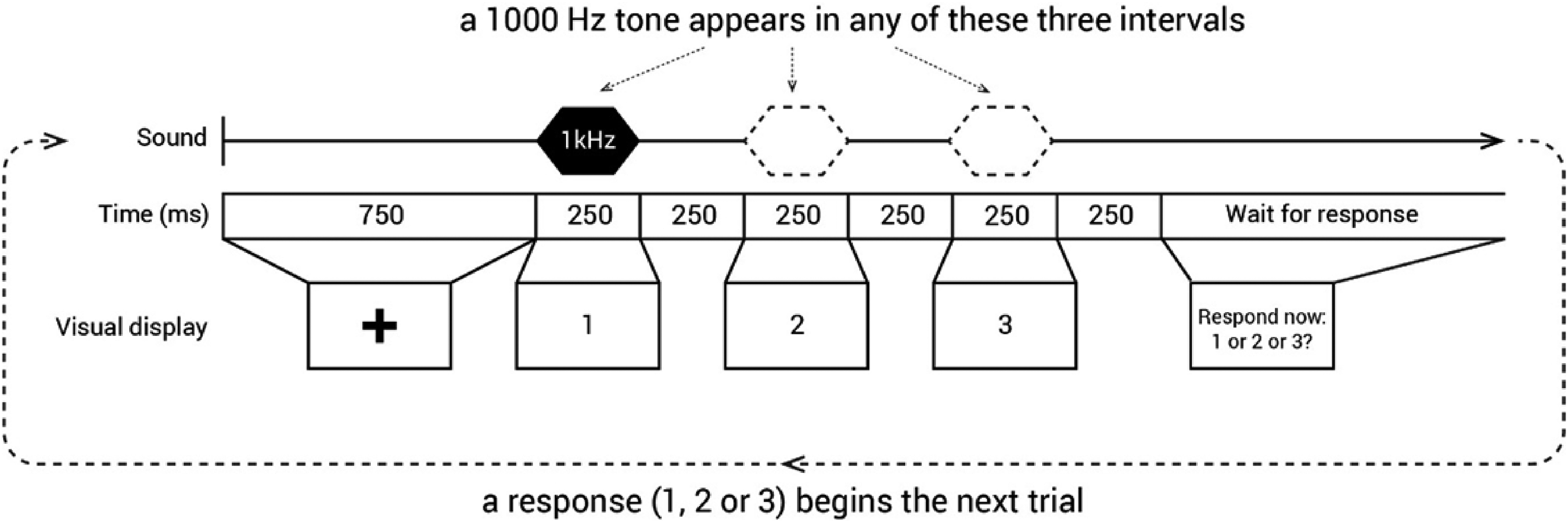
Trial structure in the threshold staircase procedure. In Expt 2, only one of the three intervals (1, 2, or 3) contained the signal, a 250 ms, 1 kHz pure tone. Responses were collected by participants pressing the corresponding numerical key on their computer keyboards.
The level of the signal relative to noise that was required to produce 79.4% correct detection was determined using an adaptive ‘three-down, one-up’ staircase procedure (Levitt, 1971). The procedure started at a signal-to-noise ratio (SNR) of −13.75 dB (calculated as dB difference in RMS between the background white noise and pure tone). Each track began with an initial descent to approximate threshold, with every correct response leading to a decrease in signal intensity by 1.5 dB with the decrement reducing to 0.75 dB once the level fell below −19.75 dB SNR or after the first incorrect response. At this juncture, the three-down, one-up staircase procedure started.
As practice before the first of three adaptive threshold staircase tracks, participants completed six trials with the signal presented at −13.8 dB SNR (i.e., the easiest level) and with performance feedback provided (“correct” or “wrong” shown for 1 s on-screen after each response). The average performance of this practice block was 92.78% correct (SD = 13.85%) with 41 out of 60 participants (68%) making no mistakes. No feedback was given during the adaptive staircase threshold session.
Each of the subsequent three adaptive staircase threshold tracks consisted of 40 trials. Tracks were completed consecutively, with the opportunity for a short break between tracks. However, most participants did not take a break (mean break duration = 9.03 s, SD = 11.68 s).
To keep participants engaged throughout the procedure, progress was shown on the top left of the screen (“Progress: x/40”, where x is the index of the current trial). Moreover, we awarded a bonus (maximum of £1.50) in addition to the base payment; after the 6 practice trials with feedback, participants were informed that if their accuracy surpassed 50%, they could earn a bonus of 50p per track. The accumulated bonus was shown at the end of each track, and all 60 participants got the full bonus of £1.50.
The threshold staircase procedure was achieved using in-house code [https://gitlab.pavlovia.org/sijiazhao/threshold_demo].
Assessment of Participant Apathy, Motivation, and Fatigue
To measure lack of motivation (apathy), we presented the Apathy Motivation Index (AMI) questionnaire before the experiment. This 18-question survey is subdivided into three apathy subscales: emotional, behavioral and social apathy (Ang et al., 2017; see Supplemental Materials for questions).
To track the dynamics of motivation and fatigue across the experiment, participants also rated their level of subjective motivation, fatigue, and confidence before and after the threshold session. They were provided with three horizontal visual analog scales, each with equally spaced tick marks along its axis, an accompanying question positioned centrally above, and labels at the extreme left and right of the scale. The questions and labels are available in Supplemental Materials.
Responses were registered by a click on the appropriate position on each scale. After completing all three ratings, a ‘confirm’ button appeared at the bottom of the screen, allowing participants to submit their ratings.
The questionnaire and ratings were added to the experiment on the second day of data collection. Thus, of the 60 participants, 49 responded to both the AMI questionnaire and ratings of motivation and fatigue, 10 had the AMI questionnaire only, and a single participant completed neither the questionnaire nor the ratings.
On average, participants spent 39.3 min (SD = 10.4) on the entire experiment, including both the Adaptive Staircase Threshold procedure (Expt 2) and the Probe Signal procedure (Expt 3, below).
Results
Reliability of Individual Participant Signal-to-Noise Thresholds in Online Psychophysical Staircase Procedure
First, we asked whether we could obtain good-quality and stable tone-in-noise thresholds online. As an initial qualitative approach, we examined the three 40-trial tracks for each participant. We found that they were generally well-behaved in terms of reaching a stable plateau with multiple reversals after the initial descent to the first error. (All threshold tracks are available at https://github.com/sijiazhao/TPS_data). To estimate threshold distribution and reliability across tracks, we calculated the mean and range of thresholds for each participant, based on the last six reversals for each of the three tracks unless that track had fewer than six reversals. (Mean reversals across tracks was 7.8. Sixteen participants had one track with fewer than 6 reversals: 2 tracks with 3 reversals, 1 track with 4 reversals, 13 tracks with 5 reversals). The mean SNR threshold was −19.54 (SD = 1.39), with the distribution of mean thresholds slightly skewed toward lower SNR levels (see Figure 6(a)). The mean range of estimated thresholds across the three tracks was 1.71 dB (see Figure 6(b)); with a 10th and 90th percentile range of 0.39 to 3.41 dB SNR. A repeated-measures ANOVA on the mode-based threshold for each track showed no significant order effect [F(2,118) = 2.30, p = .11, partial eta squared = 0.038, observed power = 0.46, no significant violations of sphericity, so sphericity assumed].

Results from expt 2. (a) Frequency histogram of all participants’ tone-in-noise thresholds in dB SNR based on the mean of the SNR values of the last six staircase reversals (count on y-axis). (b) Frequency histogram showing the distribution of the range of 6-reversal-based thresholds across the three thresholding tracks (in dB SNR). (c) The violin plots for the tone-in-noise detection thresholds across 60 participants estimated using the four estimation methods. Each violin is a kernel density plot presenting the distribution of the estimated thresholds for each estimate method. For each violin plot, the group’s median (the horizontal black line inside the violin), interquartile range (the vertical box) and 95% confidence interval (the vertical black line) are shown.
Evaluation of Mode-Derived Thresholds Compared to Reversal Counting
We compared four different methods of deriving a threshold from psychophysical data collected in the 3-down/1-up adaptive staircase procedure. The goals were: 1) to determine whether reliable threshold estimates could be obtained using fewer trials; 2) to examine whether the statistical mode is a viable alternative to the standard approach (the mean across a predetermined number of reversals).
One approach to establishing a threshold is to average values at the last six reversals in each of three tracks, and to compute a grand mean 'gold standard' threshold for each participant from these three-track means (green violin in Figure 6(c)). Another is to estimate a threshold from the psychometric function reconstructed from all 120 trials using maximum likelihood procedures carried out in the psignifit toolbox in MATLAB (Schütt et al., 2016; pink violin plot in Figure 6(c)). We also calculated the statistical mode for all 40 trials in each of the three tracks per participant, and generated a grand mean from these three modal values for each participant (orange violin in Figure 6(c)). The rationale for using the mode is that it can be thought of as a measure of the ‘dwell time’, e.g., how long a participant spends at a particular level in the adaptive staircase procedure. Finally, we computed the mode from the first 20 trials in each participant's first track in order to assess the goodness of a mode-based threshold estimate from a single short track (purple violin in Figure 6(c)). On average, the number of reversals when the 20th trial was reached in the first track was 3.5 (SD = 1.0).
We compared these four metrics using a Bayesian repeated measures ANOVA in JASP (JASP Team, 2020; Morey and Rouder, 2015; Rouder et al., 2012), which revealed a very low Bayes factor compared to the null hypothesis (BF10 = 0.592), as would be expected given the ≤ 0.2 dB SNR mean difference between any of the four metrics. This suggests that there is little, if any, significant bias in using either modal measure versus the more standard approaches.
However, a potentially more consequential difference between obtaining a single 20-trial threshold track estimate versus using the three-track 40-trial 6-reversal-based estimate would be unacceptably high variability in the former case. To quantify the degree of variability associated with the number of trials used to calculated the threshold, we compared the distributions of differences between the 3-track grand average and single-track thresholds calculated using the mode of 1) the first 20 trials; 2) or 30 trials; 3) all 40 trials; or 4) the mean of last six reversals. Each participant contributed 3 difference scores (one per track) to each distribution. Figure 7 shows the range of deviation from the gold-standard that is observed when using mode-based estimation. As would be expected, dispersion decreases as more trials are used to calculate the threshold.

Difference in db SNR of each participant's single tone-in-noise threshold tracks derived from the mode of the first 20, 30 and all 40 trials along with the mean of the last six reversals when compared to the 'gold standard' mean of three reversal-based thresholds. Note that each participant contributes three datapoints (one from each track) to each distribution.
We also assessed the adequacy of single-track mode-based threshold estimates using the initial 20, 30, or all 40 trials. To do so, we examined the correlation of each mode-based threshold with the 3-track threshold across participants, and then statistically compared the difference in correlations. As tested using the r package cocor using the Hittner et al. and Zou tests (Diedenhofen & Musch, 2015; Hittner et al., 2003; Zou, 2007), the fit between the gold standard and mode-based thresholds differed across tracks 2 (Figure 8, r-values shown in figure). Here, the correlations between each mode-derived threshold from first thresholding track and the gold standard threshold were all significantly (p < .05) lower compared to when the same measure used data from the second thresholding track. Correlation differences between the first and third tracks were in the same direction, but 'marginal' using the Hittner et al. tests (p < .08). The less-robust thresholds obtained in the first track suggest that at least some psychophysics-naive online participants had not quite acclimated to the threshold setting procedure until later on in the track.

Correlations between the 3-track gold standard threshold (y-axis) and single-track threshold estimates (x-axis) based on the mode of the first 20, 30, or all 40 trials (track 1 (left), 2 (middle), and 3 (right panel)). Light green crosses and lines refer to 20-trial mode estimates, dark green to the 30-trial estimates, and purple to the 40-trial estimates. Both axes show tone-to-noise dB SNR. Pearson’s correlation coefficients for each estimate are shown on the right of the fits.
Using the same difference-in-correlation-based comparison method (and with the same statistical caveats), we also found that the relative reliability of mode-based thresholds derived from 20 or 30 versus 40 trials changed across tracks. In the first and second tracks, thresholds based on the first 20 trials were significantly less correlated with the gold standard than were those based on 40 trials (p < .05) but did not differ in the last track; correspondingly, first-track thresholds based on the first 30 trials were significantly less correlated with the gold standard than were those based on 40 trials (p < .05), but this difference was no longer significant in the second or third tracks. In addition, the overall deviation of mode-derived scores from the gold-standard approach (the standard deviation of the threshold differences; SD in upper-right corner of each panel in Figure 7) decreases with increasing number of trials, indicating a convergence of the mode-based threshold approaches toward the gold standard. A reasonable explanation for this effect is that online participants acclimated to the threshold setting procedure across the three tracks, and performance became more stable and consistent after a few minutes of practice. Nevertheless, as shown previously (Figure 8) even tone-in-noise thresholds based on the first 20 trials in the first track are reasonably accurate estimates of a participant’s ‘true’ threshold.
Evaluation of Potential Motivation, Confidence, and Fatigue Effects on Tone-in-Noise Thresholds
Here, we asked whether estimated thresholds might in part reflect the personal motivation of online participants. To this end, we used a common self-report for a personality trait-like component of motivation among healthy populations (apathy in the AMI questionnaire, Ang et al., 2017). We also examined the dynamic change of motivation ratings across our task, measured before the first threshold track and again after the third threshold track.
Participants’ tone-in-noise thresholds from did not correlate with any aspect of the motivation trait measured by the AMI questionnaire. Neither behavioral (rho = .055, p = .68), emotional (rho = .079, p = .55), nor social apathy (rho = .053, p = .69) dimensions were related to tone-in-noise thresholds. Self-reported motivation across the course of the staircase thresholding procedure also did not account for threshold level either before (rho = −0.15, p = .29) or after (rho = 0.007, p = .96) the threshold procedure.
To assure ourselves that this lack of correlation was not due to a faulty instrument, we tested whether there was a correlation between the trait motivation/apathy score and the in-experiment motivation ratings. Indeed, the behavioral dimension of the apathy questionnaire was associated with the post-experiment motivation level (rho = −0.37, p = .010) and this relationship remains significant after controlling for the threshold level (partial correlation, r = −0.39, p = .006). This indicates that more apathetic individuals reported feeling less motivated after the threshold session regardless of their behavioral performance, although no relationship was observed prior to the experiment.
The absence of a link between motivation and task performance was further confirmed by a repeated measures general linear model on the tone-in-noise threshold level with fixed effects of the total score of the apathy questionnaire, the pre-threshold and the post-threshold motivation ratings. The thresholds could not be predicted by apathy traits (F(1,41) = 0.022, p = .88), or motivation ratings either pre-experiment (F(1,41) = 0.93, p = .34) or post-experiment (F(1,41) = 0.15, p = .71). Moreover, there were no three-way or two-way interactions (all p > .32). In sum, online participants’ motivation did not contribute significantly to their tone-in-noise thresholds.
Threshold level was also not significantly related to confidence measured either before (rho = 0.074, p = .61) or after the experiment (rho = −0.12, p = .40), suggesting that participants showed quite limited metacognitive awareness of their performance.
Finally, we investigated the relation of self-reported fatigue to thresholds. Here, the threshold level did positively and moderately correlate with fatigue ratings both before (rho = 0.31, p = .027) and after (rho = 0.32, p = .025) the experiment, consistent with higher (poorer) thresholds among fatigued participants.
In all, Expt 2 demonstrates that it is possible to quickly and reliably estimate a classic auditory psychophysics threshold online. Moreover, a very simple -- and easily automatized -- estimate of the level at which participants dwell for the most trials across the adaptive staircase procedure (the mode) is highly reliable, and as robust at estimating threshold as traditional estimators based on staircase reversals. We outline potential usage cases regarding the number of tracks and trials to use in the Discussion. Finally, online participant motivation level is not a significant moderator of tone-in-noise perceptual threshold (at least within the range of motivation levels and task difficulty we measured here), whereas fatigue was associated with somewhat poorer tone-in-noise detection.
Experiment 3
Experiment 3 tests an online version of the classic probe signal paradigm to measure frequency-selective auditory attention (Borra et al., 2013; Dai & Buus, 1991; Dai et al., 1991; Green & McKeown, 2001; Greenberg & Larkin, 1968; Macmillan & Schwartz, 1975; Moore et al., 1996; Scharf et al., 1987). We ask 1) whether the Expt 2 online tone-in-noise threshold-setting procedure is sufficient for setting the SNR level to achieve a specific target accuracy in the 2AFC tone detection task used in the probe signal paradigm. We then ask 2) whether this paradigm can be replicated online in relatively uncontrolled environments; 3) if frequency-selective attention effects can be observed on an individual basis within a single short online testing session (circa 30 min); and 4) if these effects change across the course of a testing session. As with Expt 2, we finally ask 5) whether psychophysical thresholds and frequency-selective attention are related to well-established measures of fatigue, apathy, and task confidence before, during, or after testing.
Methods
Participants
All participants from Expt 2 also took part in Expt 3.
Stimuli and Procedure
Like Expt 2, Expt 3 was implemented using PsychoPy v2021.1.2 and hosted on PsychoPy’s online service, Pavlovia (pavlovia.org). A demo is available at [https://run.pavlovia.org/sijiazhao/probesignal_demo]. All experimental restrictions used in Expt 2 also applied in Expt 3.
After completing the Amplitude Setting, Headphone Check, and Threshold Setting of Experiment 2, participants completed a classic probe-signal task (Anandan et al., 2021; Botte, 1995; Dai & Buus, 1991; Dai et al., 1991; Greenberg & Larkin, 1968; Scharf et al., 1987; Tan et al., 2008). Continuous broadband noise was present throughout all trials, as described for the threshold setting procedure.
As shown in Figure 9, each trial began with a 1000 Hz, 250 ms cue tone followed by 500 ms of silence. At this point, the first of two listening intervals was indicated by a black ‘1’ presented at central fixation on the white computer screen for 250 ms. The ‘1’ disappeared during a 250 ms silent interval at which time a black ‘2’ was presented at fixation to indicate a second listening interval.
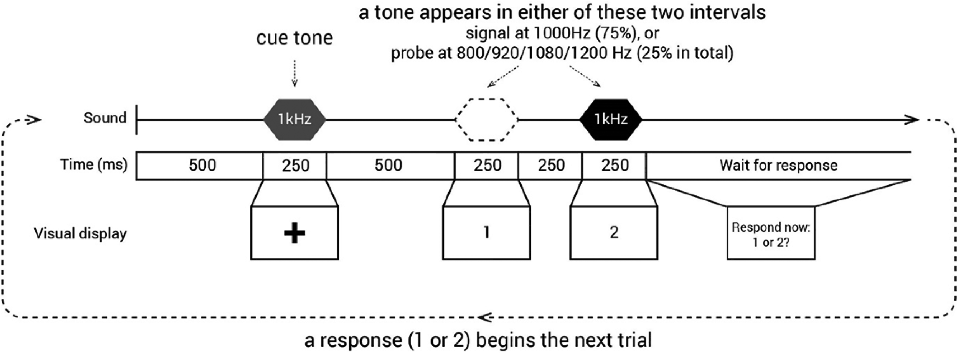
Trial structure in the probe signal task. In Expt 3, one of the two intervals (1, 2) contained the signal, a 250 ms, 1 kHz pure tone. Responses were collected by participants pressing the corresponding numerical key on their computer keyboards.
A 250 ms tone was presented with equal probability in either the first or the second listening interval; participants reported which interval contained the tone with a keypress. Signal trials involved a tone that matched the 1000 Hz cue frequency; these trials comprised 75% of the total trials. Another four probe tones with 800, 920, 1080, and 1200 Hz frequencies were presented with equal probability across the remaining 25% of trials (6.25% likelihood for each tone frequency).
To assure ourselves that the full sample did not perform at ceiling, we adjusted each individual's probe-signal SNR threshold slightly, lowering it by one step size (0.75 dB) from the threshold estimated in Expt 2. The signal and probe tones were always presented at the adjusted threshold level; the preceding cue tone was suprathreshold, set at 14 dB above the adjusted threshold SNR level.
Participants first completed five practice trials with suprathreshold signal and probe tones presented at −13.8 dB SNR. Immediately thereafter, another five practice trials involved signal and probe tones at the adjusted individual threshold. Performance feedback (‘correct’ or ‘wrong’) was provided on-screen for one second following each response to a practice trial.
Each of the subsequent 12 blocks consisted of 32 trials (384 trials total), with 24 signal trials (1000 Hz tone) and 2 probe trials at each of the other frequencies (8 probe trials total) in random order. Blocks were completed consecutively, with the opportunity for a short break between blocks (mean break duration = 10.44 s, SD = 22.44 s). There was no feedback for these trials.
Participants were informed that if their overall accuracy across the 12 blocks surpassed 65%, they would earn a bonus of £1.00 at the end of the experiment. In all, 63% of participants earned the bonus.
Results
Adequacy of Online Thresholding for Setting SNR Levels for 2AFC Task
We first asked how effective the online tone-in-noise threshold measurement was in setting the SNR level for the probe signal task. The adaptive staircase procedure (3-down, 1-up) was designed to set the threshold to detect a 1000 Hz tone in noise at 79.4% accuracy. However, to retain additional 'head room' for accuracy in the probe signal task we lowered the actual SNR level by 0.75 dB for each individual (as noted above). In order to map how changes in tone-in-noise SNR levels mapped to changes in 2AFC tone-in-noise detection accuracy, we ran a small study and found that each 0.75 dB increment in SNR corresponded to a detection accuracy change of 4.2%. Thus, if the Expt 2 online threshold setting functioned correctly, Expt 3 participants should achieve tone-in-noise detection of 75.2%. As shown in Figure 10(a), average signal detection accuracy was 72.45% (SD = 8.86), just slightly (2.75%) yet significantly lower than the predicted accuracy (t(59) = 62.67, p < .001, BF > 1050).

Experiment 3: probe-signal (n = 60). (a) Distribution of the signal accuracy using the mode-derived threshold. The population mean is labeled as a dash vertical line. (b) The percentage correct detection of 1000 Hz signal and each of the four probes (800, 920, 1080 and 1200 Hz). The thick black line presents the group mean, with error bar = 1 SEM. Each gray line indicates individual data. (c) The accuracy to detect signals (highly probable 1000Hz tones) was significantly higher than the average detection accuracy for probe tones (the less probable 800, 920, 1080, and 1200Hz tones) The population data is presented as a boxplot with the outliers marked as gray crosses. Each gray line indicates individual data, and paired t-test stats reported below the graph. The RT data is shown in the same manner below, d, e and f. For the visualization, the individual data are not presented in (e), but a summary of individual data is shown in (f).
If the Expt 2 mode-derived threshold adequately estimated tone-in-noise thresholds, then a participant's tone-in-noise detection accuracy in Expt 3 should be independent of their tone-in-noise threshold. In other words, even if two participants have very different tone-in-noise thresholds, their accuracy on the 2AFC probe-signal task should be more or less equivalent. Indeed, probe-signal detection accuracy was not correlated with the mode-derived threshold level (Spearman rho = −0.08, p = .544; Pearson r = −.01, p = .929).
Robustness of the Probe-Signal Effect at Group and Individual Level
As shown in Figure 10(b), online participants detect the high-probability 1000 Hz signal at levels that are approximately at the predicted target accuracy (72.45% (SD = 8.86), Figure 10(a) and (c)), whereas tones with less-probable frequencies are much less accurately detected (53.59% (SD = 5.36), Figure 10(c)). Figure 10(c) plots a direct comparison of what is visually apparent in Figure 10(b). The signal tone was detected significantly more accurately than were probe tones (t(59) = 13.82, p < .00001, BF > 1017; Figure 10(c)). This classic pattern of frequency-selective auditory attention is echoed in faster reaction times for the 1000 Hz signal tone compared to the probe tones (t(59) = 6.77, p < .00001, BF > 106; Figure 10(e) and (f)). These results replicate the frequency-selective attention effects that have been documented in laboratory studies for decades (Anandan et al., 2021; Botte, 1995; Dai & Buus, 1991; Dai et al., 1991; Green & McKeown, 2001; Greenberg & Larkin, 1968; Moore et al., 1996; Scharf et al., 1987; Tan et al., 2008) using a naive online sample of participants who utilized variable consumer equipment in uncontrolled home environments. This effect was notably robust even at the individual participant level: 56 of the 60 participants (93.33%) showed at least a 5% detection advantage for signal versus probe frequencies. Moreover, the effect of the high-probability signal was established rapidly among naïve listeners. This supports models of frequency-selective attention dependent upon a system that adjusts very rapidly to input regularities (Fritz et al., 2003; Hafter et al., 1993).
Time Course of the Probe-Signal Effect
Here we asked how the probe-signal effect may change as participants become more practiced over time. As in the literature, we calculate the probe-signal effect as the difference between accuracy for the most probable frequency (the 'signal') and average accuracy for the least probable frequencies (the 'probes’ in Figure 11(a)). A linear mixed-effect model (LMM) using block index as a fixed effect and participants as a random effect showed that the probe-signal effect diminished slightly as the task progressed (F(1,718) = 7.87, p = .0052). This result was mirrored in RTs (Figure 11(b)); although response times to both signal and probes decreased over time, the difference between the two was overall smaller at the end of the experiment (LMM, effect of block index: F(1,711) = 10.75, p = .0011).
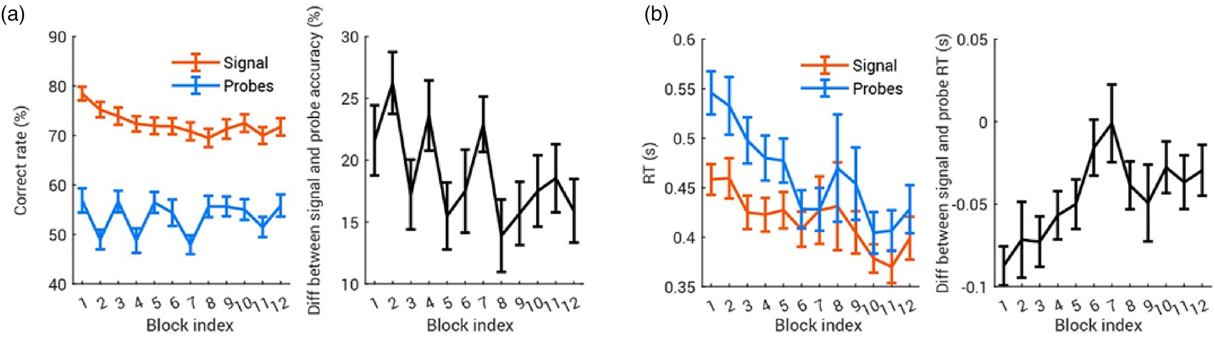
Dynamics of the probe-signal effect. In all plots, the error bar shows ± 1 SEM. (a) Probe-signal effect in accuracy decreased over time. In the left panel, signal and probe accuracy are computed for each block and averaged across participants. The probe-signal effect is computed as Signal Accuracy - Average Probe Accuracy; the group average probe-signal effect is plotted in black in the right panel. (b) Probe-signal effect in RT is shown in the same manner; RT to signal and probe tones are plotted against the block index, with their difference is shown in the right panel. Note that since the probe-signal effect in RT is computed as RT-to-signal minus RT-to-probe, more negative values mean larger probe-signal effects.
Effect and Time Course of Motivation Variables Across the Probe-Signal Experiment
During the 12-block probe-signal task, participants were instructed to rate how well they felt they performed, how motivated they were, and how tired they felt at the end of each block. This allowed us to examine how the probe-signal effect evolves along with individuals’ dynamics of confidence, fatigue and motivation.
As would be expected given the difficulty of the probe signal task, confidence remained low throughout (Figure 12(a)). An LMM on confidence rating showed that as the task progressed, confidence decreased slightly, but not significantly so (F(1,595) = 3.50, p = .062), with higher confidence associated with better overall accuracy (F(1,595) = 5.21, p = .023). With increasing time on task, fatigue accumulated (Figure 12(b), LMM on fatigue with block and accuracy, effect of block: F(1,595) = 47.01, p < 10−10) and motivation diminished (Figure 12(c), LMM on motivation with block and accuracy, effect of block: F(1,595) = 59.36, p < 10−13). However, ratings of fatigue and motivation were not significantly related to the probe signal performance of that block (LMM with block and accuracy, effect of overall accuracy on fatigue: F(1,595) = 0.32, p = .57; effect of overall accuracy on motivation: F(1,595) = 1.06, p = .30).

Dynamics of confidence, fatigue, and motivation across the probe signal experiment. In all plots, the error bar shows ± 1 SEM.
Finally, to investigate the effect of motivation and fatigue on the probe-signal accuracy effect, we ran an LMM with block index, motivation rating and fatigue rating as fixed effects and participants as a random effect. 3 While fatigue did not show an influence on the probe-signal effect (F(1,594) = 0.067, p = .80), the probe-signal effect decreased over blocks (F(1,594) = 5.54, p = .019) and increased slightly with motivation (F(1,594) = 5.61, p = .018). This suggests that a larger probe-signal effect is predicted by high motivation, but not low fatigue.
Discussion
Here, we developed and tested new approaches to making auditory psychophysical methods viable for online studies with psychophysics-naive participants. We first showed that the problem of limiting the range of stimulus sound levels can be addressed by using each participant as their own reference for setting stimulus levels at a given dB RMS above their noise detection threshold. We then showed that online participants’ perceptual tone-in-noise thresholds could be reliably estimated, not only by combining data from multiple tracks as is classically done, but also with a single short staircase track with a simple mode-based analysis that is easily implemented even by novice researchers. Individual differences in online participants’ apathy, confidence, and motivation did not significantly influence their perceptual thresholds, although those who were more fatigued tended to show somewhat less-sensitive thresholds. Online tone-in-noise thresholds also were reasonably reliable in setting the desired accuracy level for a new online version of the classic probe-signal task (Dai & Buus, 1991; Dai et al., 1991; Greenberg & Larkin, 1968; Moore et al., 1996; Scharf et al., 1987). Moreover, despite using only a third of the trials of a recent and efficient in-lab version (Anandan et al., 2021), we found a robust frequency-selective auditory attention effect overall, and in 93% of individual participants. This compares well with results from studies with few participants each undergoing thousands of trials. Indeed, the probe signal effect itself could be clearly detected at a group level from the first block of trials (Figure 11(a)). The magnitude of the attentional probe-signal effect decreased somewhat as the task proceeded, which was related somewhat to a decrease in motivation over time, but was not significantly associated with overall participant fatigue, or with changes in fatigue ratings over time. In sum, these experiments show that using such vetted ‘auditory hygiene' measures can facilitate effective, efficient, and rigorous online auditory psychophysics.
A Method for Remotely Setting Stimulus Amplitude Levels
The human auditory system is capable of successful sensing signals across a remarkable range of acoustic intensity levels, and many perceptual and cognitive phenomena are robust to level changes (Moore, 2013). However, a lack of control over auditory presentation levels - as is often the case in online experiments - is far from desirable on several grounds. Hearing safety is of course a potential concern for online experiments, particularly when presenting punctate sounds for which onset times are considerably faster than the ear's mechanical protective mechanisms can respond. Sounds presented at different absolute levels evoke responses in distinct auditory nerve fibers, which can be selectively affected by pathological processes (Schaette, 2014; Verhulst et al., 2018). As noted above, the frequency selectivity of subcortical and cortical auditory neurons can vary systematically as a function of sound pressure level (Moore, 2013; Schreiner et al., 2000). Of course, absolute sound pressure level is not the only factor to consider: individual participants with normal hearing will show thresholds with a range of up to 30 dB HL, and therefore a fixed absolute amplitude level can result in quite different perceptual experiences for participants who lie at one end or the other of this hearing range.
In Expts 1a-d, we found that community-recruited participants could very quickly adjust levels via the computer volume setting to estimate their hearing threshold using diotic pulsed white noise. The 20–25 dBA SPL range accords well with that of normal hearing (Park et al., 2016); and the extrapolated threshold levels are highly consistent across the outdoor settings of the three experiments. Expt 1c and Expt 1d showed that participants’ thresholds indoors and outdoors were highly correlated; this not only shows excellent reliability (albeit in a relatively small sample given the strictures of working during the COVID pandemic), but also demonstrates the robustness of this method to different acoustic environments. The spectra of both background noises have generally low-pass characteristics, so headphone attenuation should not be appreciably different; thus, we measured attenuation in only one of the backgrounds (the anechoic chamber). The fact that the thresholds were quite similar in indoor and outdoor environments, despite the large difference in ambient noise levels, may be due to the non-stationary nature of the noise, providing gaps in which the listeners could detect the presence of the signal. We plan a larger-N follow-up when in-person studies in indoor environments are more feasible than at the time of writing.
For experimenters who need to present auditory stimuli within a given range of intensities or at a particular level above perceptual threshold, the presentation level can be referenced to the RMS level of the white noise stimulus used in the amplitude setting procedure. For instance, say an experimenter wants to set her stimulus presentation level at ∼ 60 dBA SPL. an average of. If she assumes the typical participant will be in an acoustic environment similar to the outdoor setting (with an average 50 dBA SPL ambient noise level) the average stimulus soundfile RMS to produce an average 60 dBA SPL level in the headphones can be estimated. Recall that the RMS of the white noise file used in Experiment 1a (background noise level ∼50dBA) was 0.000399; using this stimulus, participants set their thresholds to an average of 29.4 dBA SPL (range 22.3–35.6 dBA SPL).
To achieve the desired average SPL of 60 dBA for the experimental stimulus, the experimenter can scale the RMS amplitude of the experimental stimulus soundfile as follows. First, calculate the difference in dbA between the desired average SPL and the SPL associated with the average participant's threshold for white noise: 60 dBA–29.4 dBA = 30.6dB SPL. Second, calculate the RMS of the experimental stimulus; for the present example, we will assume the sound has an RMS of 0.0080. Third, calculate the RMS amplitude difference in dB between the experimental stimulus (0.0080) and the white noise stimulus used for thresholding (0.000399), using the following formula: dB ratio = 20 × log10(experimental stimulus RMS / white noise RMS) = 20 × log10 (0.0080/0.000399) = 26.04dB. Fourth, calculate the difference in dB between the results of step (1) and step (3), e.g., 30.6dB minus 26.04dB = 4.54dB. Finally, scale the experimental stimulus file amplitude by this amount to achieve the desired RMS, either in an audio editing program like Audacity, or through calculation on the soundfile values itself in a program like Matlab, e.g., output_stimulus = input_stimulus × 10 ^ (4.54/20).
Assuming our Expt 1a-c noise detection threshold results generalize to the online population, the 10th and 90th percentiles of presented levels across all participants should be approximately 54- and 68-dBA SPL. Alternatively, the stimulus RMS could simply be scaled 30 dB above each individual participant's white noise threshold level to ensure that stimuli are sufficiently audible to the vast majority of participants. One very important caveat to this approach is in the case where the spectrum of experimental stimuli is far from the 1–4kHz band that will drive much of the detectability of the white noise stimulus (for instance, pure tone stimuli at lower or very high frequencies). Here, it is important that either additional checks be placed on stimulus amplitude, or that a different thresholding stimulus be used (for instance a narrower-band noise centered around the stimulus frequency).
Of course, individuals will have different laptops with different sound card characteristics, different quality headphones etc. Although we chose to use a band-limited noise as our stimulus to help mitigate these potential confounds, this does not ensure that there are no differences across subjects. Within the selected band, however, the frequency response of each participant’s setup will be constant between the amplitude setting procedure and the psychophysical test of interest, which renders across-subject differences in technology less critical, especially when common-sense steps are taken in designing each online experiment.
For example, avoiding both narrow-band stimuli like tones as well as stimuli that are not band-limited like broadband noise will limit the effects of across-subject hardware frequency response differences on results. Ensuring that subjects are working at SPLs that are reasonably above threshold will help ensure that audibility is not a confound. Better still would be to design studies in which the experimental SNR ensures that stimulus noise levels are likely to overwhelm the levels of environmental noise sources.
Asking participants to avoid using open-back headphones, and instead to use closed-back or insert phones with soft rubber or latex tips will likely help alleviate the intrusion of environmental noise on psychophysical data. To establish the potential amount of insertion loss that might be expected from closed back headphones like those used here, we placed an acoustic manikin (Knowles Electronics Manikin for Acoustic Research) in the anechoic chamber, and presented the band-limited white noise stimulus from approximately 2m away and directly in front. Recordings were made from KEMAR’s microphones with and without the Beyer Dynamics DT150 headphones used in the study, in position. We then compared the RMSv levels of each recording and found that the headphones provided about 9 dB of attenuation. We re-ran this analysis with various other headphone models that were readily available to us (as well as 3M foam ear plugs as a reference) to determine the degree of variability. These data are shown in Supplementary Materials Figure S3. Among the circumaural phones we tested, the AKG K271’s provided the least amount of attenuation, at about 6 dB, while the Beyer Dynamics used in the study provided about 9 dB of attenuation.. The two sets of supra-aural phones we tested – RadioEar DD45 and TDH-49 – provided the poorest attenuation, along with the Apple AirPods, which is not surprising given their non-pliable hard plastic shell. While far from exhaustive, this analysis suggests that even inexpensive circumaural closed-back headphones, will likely provide at least 6 dB or so of attenuation.
Time-Efficient and Reliable Estimation of Tone-in-Noise Thresholds
We used the 'amplitude-setting' method of Expt 1 with all Expt 2 participants. Based on this, the online continuous white noise masker played during both parts of Expt 2 was set to 40 dB above each participant's white noise detection threshold, resulting in an average of 66 dBA SPL (SD = 4.3). Using a standard staircase technique to estimate tone-in-noise thresholds, we were able to obtain stable threshold estimates in online participants (Figure 6), not only by using the traditional method of averaging the means of the last six reversals from three staircase threshold tracks, but also using an easy-to-calculate and robust mode of the SNR levels from the first 20, 30, or all 40 trials (Figure 7). We also found that it was possible to obtain a reliable threshold from a single track of 20 trials (Figure 8), entailing about a minute of online testing.
If a psychophysical task takes about 3 s per trial, then a standard thresholding track of 40 trials would take two minutes, and three tracks would take 6 min excluding time between tracks. Using the same assumption, the mode-of-20-trials approach would take about one minute to generate a threshold, a significant reduction in testing time. This streamlined threshold setting approach may be very attractive for online testing settings, as the vigilance of participants might not be as high as it would be during in-person testing, where experienced participants can typically be expected to generate reliable data for 1.5 h or more. This fact places a premium on time-to-threshold for online studies. However, further investigation is needed into estimation with multiple modes, with multiple tracks, or more disperse SNRs. Although in more traditional psychophysical testing scenarios, this reduced thresholding time would not be worth the corresponding increased variability associated with the mode-based approaches described here, online testing easily offers larger sample size from a more diverse population than traditional in-person testing on the university campus. Thus, it is suggested that the streamlined thresholding approach described here, along with shortened online testing sessions, and increased sample sizes can yield better, more reliable outcomes when testing online.
There are other issues to consider in maximizing the efficacy of online testing using streamlined thresholding. For example, psychophysical tasks that require participants to work near or at their thresholds-in-quiet are likely not suitable, because overall ambient sound level is less controlled in online studies (as described in Expt 1), which raises signal audibility as an issue. This adds more uncertainty by the participant to the task, which makes short, 20-trial tracks less reliable. In a similar way, tasks in which the required perceptual decision is based on subtle cue differences like those that are often categorized as timbral may not be good choices for online study, again because bad tracks are more likely. Generally, it is recommended to choose psychophysical tasks that are easy for novice listeners to understand and ‘hear out,’ and to implement a training regimen that is carefully designed to clarify the perceptual task for listeners to avoid bad tracks, which are more difficult to discern with streamlined threshold setting procedures.
Finally, another potential advantage of the mode-based approaches might lie in their ease of computation. It is undeniable that online platforms such as Pavlovia.org and Gorilla.sc make psychophysical testing accessible to many, including students and other non-experts. These novice psychophysicists may have valid and interesting scientific questions. However, they may not have algorithms at-the-ready to estimate thresholds from staircase reversals using traditional approaches, a limitation that should never be a barrier to entry into the field.
Rapid and Robust Online Auditory Psychophysics of Frequency-Selective Auditory Attention in Single Participants
The probe-signal paradigm (Borra et al., 2013; Dai & Buus, 1991; Dai et al., 1991; Green & McKeown, 2007, 2001; Greenberg et al., 1970; Greenberg & Larkin, 1968; Macmillan & Schwartz, 1975; Moore et al., 1996) would not seem to be a promising target for online research. Classic and more recent psychophysical studies have both recruited highly experienced participants for multi-day experiments with extensive tone-in-threshold measurement, multiple practice sessions, and thousands to tens-of-thousands of trials in the primary experiment, all conducted with specialized equipment in acoustically isolated laboratory settings (Borra et al., 2013; Dai & Buus, 1991; Dai et al., 1991; Green & McKeown, 2007, 2001; Greenberg et al., 1970; Greenberg & Larkin, 1968; Howard et al., 1984; Macmillan & Schwartz, 1975; Mondor & Bregman, 1994; Moore et al., 1996; Tan et al., 2008; Wright & Dai, 1994). Here, Expt 3 violated each of these experimental desiderata in a single, brief online session with psychophysically naïve participants using their own computers and headphones in uncontrolled home environments. Nonetheless, we observed a probe-signal effect in most participants, with a signal-to-probe accuracy advantage of about 20–25%, on par with the magnitude of frequency-selective attention observed in studies with tens of thousands of trials (Dai et al., 1991; Greenberg et al., 1970; Greenberg & Larkin, 1968; Macmillan & Schwartz, 1975). Despite the relatively uncontrolled online experimental setting, the probe-signal effect was apparent even in response time; participants were faster in noise at detecting the signal, as compared to probe tones.
Beyond the convenience of recruiting participants online, there is power in demonstrating psychophysical effects like the probe-signal effect in a diverse sample of psychophysically naïve participants. Rather than rely on highly expert listeners, or even naïve listeners sampled from the relative homogeneity of a university campus, Expts 2 & 3 involved a world-wide sample. Behavioral science is increasingly recognizing that human behavior sampled for convenience only across university populations may be WEIRD (Western, Educated, Industrialized, Rich and Democratic; Henrich et al., 2010), and therefore not necessarily representative of populations at large. Although there are sound reasons to expect many psychophysical paradigms to generalize beyond WEIRD samples, this assumption has not often been tested (but see McDermott et al., 2016). The present results demonstrate that, with the right approach, it is indeed feasible to successfully conduct even challenging psychophysical paradigms dependent on thresholds online, and among inexpert participants. This substantially broadens the reach of psychophysics and opens the door to the possibility of large-scale psychophysics. Here, even with modest sample sizes (that nonetheless exceed typical probe-signal samples by an order of magnitude) Expt 3 demonstrated that it is possible to observe the evolution of frequency-selective attention via the probe signal effect from the first block onward, in both accuracy and RTs.
Motivation in Online Participants
Another concern with online experimentation is participants’ motivation; low levels may result in high drop-out rates and poor task engagement and performance, in turn affecting the validity of the experimental results (Shen & Chun, 2011). Compared with online participants, those attending in person might be expected to be more motivated since they have already made the effort to visit the lab, and social evaluative stress caused by the presence of the experimenter can motivate them to some degree (Bianco et al., 2021), as in the long-documented Hawthorne effect (McCarney et al., 2007).
Meanwhile, online experiments are normally completely anonymous and without supervision, leading to a common worry that the online population might be more apathetic than in-lab participants. Because of these concerns, we expected that the estimated thresholds might, at least in part, reflect motivation level. However, the estimated thresholds in Expt 2 showed no relation with motivation, neither as expressed by the apathy index (a personality-trait-like component of motivation derived from a well-established apathy questionnaire, Ang et al., 2017), nor the motivation ratings before and after Expt 2. Similarly, in Expt 3, the self-reported questionnaire-derived apathy index, as well as its subdomains, could not explain the strong probe-signal effects observed. However, we did find a weak but significant effect of in-experiment motivation on the probe-signal effect: blocks in which listeners were more motivated generated a larger probe-signal effect. Interestingly, we also found that in motivated people, high confidence strongly prevented motivation loss over time, while in apathetic people this protective effect was diminished.
One might worry that the online threshold estimation may be affected by the on-task motivation of the participants. It is interesting that, at least that in this study, we did not observe any influence of self-reported motivation on the threshold estimation amongst the remotely tested participants. On the other hand, motivation showed a small influence on the probe signal effect. This is in line with the previous work (Watson & Clopton, 1969) which found motivation — regulated by applying electric shock on incorrect trials— increased sensitivity in a simple tone-in-noise detection task but the increase was rather small. One explanation for the absent effect of motivation on the threshold estimation here is that the effect of motivation on performance is sensitive to the length of the experiment; the probe signal experiment was longer (around 20 min) and was run after the threshold estimation (a length of around 10 min). This, with no observed effect of motivation in Expt 2, indirectly suggests an advantage of keeping experiment time shorter. In summary, any generalizations of the motivation-related findings here should be taken carefully.
Supplemental Material
sj-docx-1-tia-10.1177_23312165221118792 - Supplemental material for Robust and Efficient Online Auditory Psychophysics
Supplemental material, sj-docx-1-tia-10.1177_23312165221118792 for Robust and Efficient Online Auditory Psychophysics by Sijia Zhao, Christopher A. Brown, Lori L. Holt and Frederic Dick in Trends in Hearing
Footnotes
Acknowledgments
We thank Christi Gomez, Erin Smith, and Sydney Sepkovic for their assistance in collecting in-person data. We thank Dr. Alessandro Rinaldo, Carnegie Mellon University Department of Statistics and Data Science, for statistical consultation.
Author Contributions
Declaration of Conflicting Interests
The author(s) declared no potential conflicts of interest with respect to the research, authorship, and/or publication of this article.
Funding
The author(s) disclosed receipt of the following financial support for the research, authorship, and/or publication of this article: This work was supported by the National Institutes of Health, (grant number R01DC017734 to LH and FD, and, R21DC018408 to CAB).
Data Availability Statement
Test implementations of the amplitude setting (Expt 1) are available in JavaScript [https://gitlab.pavlovia.org/sijiazhao/amplitudechecking_demo] and Gorilla [https://gorilla.sc/openmaterials/261557]. A demo can be found on Pavlovia [![]() ].
].
The guide to implement the staircase procedure (Expt 2) is available at [https://sijiazhao.github.io/how-to-staircase/]. A demo is available on Pavlovia [https://run.pavlovia.org/sijiazhao/threshold_demo/] with publicly available in-house code [![]() ].
].
The probe-signal task (Expt 3) can be tried at [https://run.pavlovia.org/sijiazhao/probesignal_demo] and its code can be found at [![]() ].
].
Supplemental material
Supplemental material for this article is available online.
Notes
References
Supplementary Material
Please find the following supplemental material available below.
For Open Access articles published under a Creative Commons License, all supplemental material carries the same license as the article it is associated with.
For non-Open Access articles published, all supplemental material carries a non-exclusive license, and permission requests for re-use of supplemental material or any part of supplemental material shall be sent directly to the copyright owner as specified in the copyright notice associated with the article.