Sage Journals: Discover world-class research

Abstract

This paper analyses the price- and volatility-based interdependency among spot, futures, and options markets in a unified framework. The paper utilizes the vector error correction model generated under the TGARCH framework, the conventional pair-wise Granger causality test, the block exogeneity and vector Granger causality test, and Schwartz–Szakmary’s factor weights to decipher the price interdependence. The paper also uses the DCC-GARCH model to examine the existence of time-varying conditional correlation in volatility. The study finds evidence of the dependency among these three markets with a stronger leading role of spot against futures and options and significant positive/(negative) influence of the previous day’s spot/(futures) price change on options’ price change. Further, the asymmetric impact of price changes on conditional volatility is observed in the case of the spot and futures market. The results also exhibit the existence of time-varying conditional correlation among these markets with spillover effect.

Keywords

Asymmetric effect conditional correlation equilibrium futures DCC-GARCH options volatility

Background

Prior to 1991, the Indian securities market was characterized by market entry barriers, high transaction cost, pricing control, open outcry-based trading, and less efficient clearing and settlement mechanisms. Moreover, the policy framework of the government in most of the cases was regulative and restrictive in nature. It was only after the economic reforms of 1991 that the market witnessed structural transformation. These reforms include strengthening the powers of the Securities and Exchange Board of India (SEBI), establishment of a new electronic stock exchange (NSE), repealing of the Capital Issue Control Act, 1947, dematerialization of securities, modified Badla system (i.e., an indigenous arrangement to carry-forward transactions), electronic trading, etc. In spite of all these changes, the Indian government was reluctant to introduce derivatives trading until 2000 due to concerns relating to trading regulations, possibility of increased speculation, operational difficulties and real-time monitoring requirements. After the detailed regulatory scrutiny and recommendations of specific committees (i.e., the L. C. Gupta and J. R. Varma Committee), India commenced trading in derivatives in June 2000 with the introduction of index futures (Padhi, 2015). The main reason for the introduction of these contracts can be attributed to their inherent benefits with respect to improvement in market efficiency, enhancement of liquidity, stabilization of excess volatility, and contribution in discovering the efficient price of the underlying asset.

Several researchers tested these utilities after their introduction. In an investigation carried out to measure the impact of derivatives trading on spot market liquidity, Bodhla and Jindal (2008) find evidence for increase in spot market liquidity during the expiration week of derivatives contracts due to the huge volume of trade in both spot and derivatives market. On the other hand, Sehgal and Kumar (2007) suggest that options market liquidity is directly related to stock price movement. However, its association is inverse with stock market liquidity and volatility. With futures and options’ volume data, Kakati and Kakati (2007) assess the relation between spot and derivatives and discover that derivatives trading results in increased covariability among Nifty50 index stocks and higher correlation between Nifty50 stocks and derivatives trading volume.

The past inquiries that concentrate exclusively on derivatives trading and spot volatility highlight the volatility stabilizing effect of futures and options (F&O) on underlying assets (Srivastava et al., 2007), more rapid assimilation of new information into prices and decline in volatility persistency (Bandivadekar & Ghosh, 2003; Sarangi & Patnaik, 2007), improvement in quality of information flow between the markets (Mahajan & Singh, 2012) after the introduction of derivatives. The literature indicates the positive impact of derivatives on the Indian stock market in terms of increased liquidity, decline in magnitude of volatility and its persistence, thereby contributing to enhancement in efficiency.

As far as the relationship between the spot and futures markets is concerned, an ample number of studies investigate the lead–lag relationship between the two markets and find evidence for the leading role of futures by Kawaller et al. (1987), Stoll and Whaley (1990) in case of US market; Abhyankar (1995), Brooks et al. (2001) in case of the UK market; Frino and West (2002) in case of the Australian market, Thenmozhi (2002), Rajput et al. (2012), Choudhary and Bajaj (2013), Rastogi et al. (2014) in case of Indian market mainly because of the inherent benefits associated with the futures in the form of lower transaction cost, higher liquidity, etc., in comparison to the spot market. In contrast to these studies, the works of Mukherjee and Mishra (2006), Misra et al. (2006), Ekta (2013), Pandey (2014), Pathak et al (2014) and Avinash and Mallikarjunappa (2017) upheld the leading role of spot over futures market in case of Indian bourse.

From a foreign options market perspective, numerous studies examine its role in discovering the price of underlying stock or index. On the one hand, Manaster and Rendleman (1982), Bhattacharya (1987), Boyle et al. (2002), Chakravarty et al. (2004), and Ni et al (2008) suggest that the options market leads the underlying asset market in absorbing information and in price discovery; on the other hand, Easley et al (1998), Chan et al (2002) and Holowczak et al (2006)’s findings reverse the inference. From the Indian context, there is no published literature available on the price relationship between the spot and options markets.

Furthermore, there is very limited literature that documents the collective influence of spot, F&O in performing price discovery functions as well as examining volatility behavior. Using five-minute interval trading costs and volume data, Fleming et al. (1996) analyze the price discovery role of spot, F&O, and find evidence for no price relationship between spot and options market relating to individual stocks. In the case of index derivatives, their findings reveal clues about the price discovery role played by both the options and futures markets. Likewise, Jong and Donders (1998) examine the lead–lag relation among these three markets using auto and cross-correlation measures. They find that the futures return leads both options and stock index returns, whereas the lead–lag relation between the cash index and the options is largely symmetrical. From the Indian market perspective, no study examined the interdependence of these three markets, except Kakati and Kakati (2007), who report the findings only on the basis of the correlation between three markets.

Through the review of the literature, we identify research gaps pertaining to two aspects. First, as studies with respect to price and volatility dependency between spot and options markets are scarce in both Indian and global contexts, there is a necessity to examine the same due to the preference given by informed traders toward the options market (Augustin et al., 2018; Black, 1975; Chakravarty et al., 2004; Cremers et al., 2015; Pan & Poteshman, 2006). Furthermore, studying the Indian spot and options markets post-US economic crisis is highly effective due to the progressive changes witnessed in terms of regulations and participation of various market players after the crisis (NSE, 2015). Second, we verify the collective influence of spot, futures, and options market on each other mainly because keeping one of the markets in isolation and then studying their influence on the spot market may make the study less accurate. In the backdrop of these gaps, we frame the following three research questions.

Whether spot, futures, and options markets exhibit price interdependence?

Do they respond differently to distinct innovations in the market?

Whether volatilities in these markets reveal a dynamic association with spillover effect?

The price interdependence among these markets is examined on the basis of a market’s ability to correct disequilibrium error, the speed of error correction, nature of influence of past prices via block exogeneity and VEC Granger causality (BEVGC) test, and pair-wise test. The relative interdependence of these markets is measured with the help of Schwartz and Szakmary’s factor weights. The study explores the volatility interdependence with a focus on evaluating how these three markets react to positive and negative return shocks induced by various market events, besides assessing the impact of past innovations and volatility persistency. An examination of the existence of conditional correlation from the context of volatility is also carried out to discover the extent and nature of association among these markets using a multivariate GARCH technique. The emergence of India as the fastest-growing major economy (IMF, 2021) and NSE as the world’s largest equity derivatives market in terms of transaction volume (Futures Industry Association, 2022) accompanied by the strong regulatory framework, diverse product offerings, market microstructural innovations, robust technological infrastructure and increased participation of retail investors makes Indian market the best fit for not only examining and deciphering the price and volatility interdependence but also generalizing the results and findings to other emerging markets and developing economies to strengthen their market.

The remainder of this investigation is planned as follows. The nature and characteristics of the dataset used in the study are described in the next section. Section 3 elucidates various methodologies and empirical approaches used to examine the relationship between spot and index derivatives markets. A detailed discussion on the results of the study is presented in Section 4, and Section 5 provides a summary of findings, implications, and concluding remarks.

Dataset

To determine the interdependence between spot and equity index derivatives markets from the Indian context, we choose the benchmark index of the Indian equity market, NSE Nifty50 as a sample asset. The index represents 13 sectors of the Indian economy, and it is comprised of F&O contracts, onshore, and offshore exchange-traded funds and other index funds. The index is also listed at the Singapore Exchange Limited and at the Chicago Mercantile Exchange. As per the “Derivatives Survey” carried out by the World Federation of Exchanges, the Futures Industry Association and the International Options Market Association, Nifty50 was declared as the most actively traded contract in the year 2015 across all diversified range of products and consistently in top 10 list since 2006 (National Stock Exchange of India, Limited, 2016). Several researchers also utilize the Nifty50 index as a proxy for the Indian capital market in their empirical studies (Debasish, 2009; Dimitriou et al., 2013; Ota, 2003). Hence, we use the daily closing price data of the Nifty50 index and its F&O contract details extracted from the historical archives of NSE for the period between January 2011 and June 2021.

In case of options, we derive the implied strike prices based on the weights of open interest (OI) of call and put option contracts by modifying Bhuyan and Chaudhury (2005) model with the Marshall–Edgeworth’s weighted index method. The reason for using OI as a weighting parameter is attributed to the informed market players’ preference argument (Augustin et al., 2018; Black, 1975; Chakravarty et al., 2004; Cremers et al., 2015; Pan & Poteshman, 2006). When these participants take a position in options at a particular strike price based on their expectation about the future price of the underlying stock, the corresponding OI measure will be increased by the number of contracts that they buy/sell. By weighting the strike price with OI, we could utilize the collective belief of each informed player about the future expected price of the stock. We use the following model to derive the implied strike price of options using OI as a weighting function:

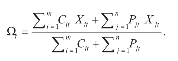
Ω_{t} = \frac{\sum_{i = 1}^{m} C_{i t} X_{i t} + \sum_{j = 1}^{n} P_{j t} X_{j t}}{\sum_{i = 1}^{m} C_{i t} + \sum_{j = 1}^{n} P_{j t}} .

(1)

Here, Ω_t represents OI-weighted strike price for each trading day. C_it and C_jt are the values of OI at ith and jth strike price on a trading day t. m and n depict the number of nonzero OI positions for calls and puts, respectively.

We further screen the data for any outliers or missing values and based on this we eliminate five days’ data from our sample period. Finally, we arrive at a total of 2,347 daily observations after matching spot, F&O data. We proceed further in investigating the interdependence between spot and equity derivatives using a group of econometric approaches which are delineated in the next section.

Empirical Approach

To examine the price and volatility interdependence, we first put the log-transformed daily closing prices of the Nifty50 index, its corresponding futures closing prices, and the daily options strike price derived from the distribution of OI (Bhuyan & Chaudhury, 2005) to test for stationarity and to figure out the order of integration using the Augmented Dickey–Fuller (ADF) test. Based on the results of the ADF test, we choose the relevant lag length for running the Johansen cointegration test and the vector error correction model (VECM) on the basis of VAR (vector autoregressive) lag length selection criteria.

After performing all these pretests, we study the price interdependence based on the speed of adjustments and lagged coefficients of endogenous variables modeled on VECM. The negative and significant speed of adjustment coefficient of VECM indicates that the dependent variable adjusts itself to reinstate the equilibrium relationship with the independent variables in the long run. VECM system specifications used in this investigation are described in equations (2), (3), and (4):

Δ S_{t} = α_{s} + β_{s} υ_{t - 1} + \sum_{i = 1}^{p} γ_{s ​, i} Δ S_{t - i} + \sum_{i = 1}^{p} δ_{s, i} Δ F_{t - i} + \sum_{i = 1}^{p} θ_{s ​, i} Δ O_{t - i} + ϵ_{s ​, t},

(2)

Δ F_{t} = α_{f} + β_{f} υ_{t - 1} + \sum_{i = 1}^{p} γ_{f ​, i} Δ S_{t - i} + \sum_{i = 1}^{p} δ_{f ​, i} Δ F_{t - i} + \sum_{i = 1}^{p} θ_{f ​, i} Δ O_{t - i} + ϵ_{f ​, t},

(3)

Δ O_{t} = α_{o} + β_{o} υ_{t - 1} + \sum_{i = 1}^{p} γ_{o ​, i} Δ S_{t - i} + \sum_{i = 1}^{p} δ_{o ​, i} Δ F_{t - i} + \sum_{i = 1}^{p} θ_{o ​, i} Δ O_{t - i} + ϵ_{o ​, t} .

(4)

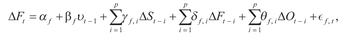
Here, the dependent variables, ΔS_t, ΔF_t and ΔO_t are the first differenced values (return series) of the Nifty50 spot price, futures price, and OI-weighted strike price, respectively. α_S, α_f and α_o represent the intercept term of the above system equations. ΔS_{t – i}, ΔF_{t – i} and ΔO_{t – i} are the lags of first differenced spot price, futures price, and options strike price and γ, δ and θ are their coefficients. υ_{t –} ₁ is the speed of adjustment term and its value depends on the cointegrating relationship among the three endogenous variables (i.e., S, F, and O). The speed of error correction term in each system equation with the coefficient β indicates how quickly the dependent market adjusts itself in correcting the disequilibrium error. The residuals of the spot equation are ∈_{S, t} and that of the futures equation are ∈_{f, t} and options equation are ∈_{o, t}. Each of these residuals is used in measuring the volatility interdependence among spot and F&O markets. We check the robustness of VECM estimation using standard residual diagnostics test and AR roots polynomials. The short-run dynamics of endogenous variables (i.e., lags of first differenced S, F, and O) are tested using the conventional pair-wise test and the block exogeneity and VEC Granger causality (BEVGC) test; the statistical significance of these variables confirm the feedback relation among the three markets.

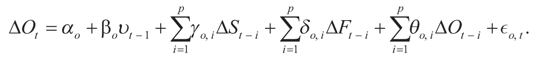
We check the robustness of VECM estimation using standard residual diagnostics test and AR roots polynomials. The relative price interdependence of these markets is analyzed using the mechanism introduced by Schwarz and Szakmary (1994) based on speed of adjustment coefficients. Their common factor weight model for futures and spot markets is described in equation (5).

ξ_{f} = \frac{β_{S}}{β_{S} + | β_{F} |} and ξ_{s} = \frac{| β_{F} |}{β_{S} + | β_{F} |}

(5)

As per Schwarz and Szakmary (1994), if the value of ξ_f = 1, then it is an indication that the price discovery process takes place in the futures market, and if ξ_f = 0, the process occurs exclusively in the spot market. We modify these common factor weights to match them to the three market scenarios with a simple and composite comparison of the price discovery function of the spot, futures, and options markets. The applied version of the composite comparison on the basis of equation (5) is described below:

Futures Spot and options - - - - - - - - ξ_{f} = \frac{β_{S} + β_{o}}{β_{S} + β_{o} + β_{F}}

(6)

Options Spot and futures - - - - - - - - ξ_{o} = \frac{β_{S} + β_{F}}{β_{S} + β_{o} + β_{F}}

(7)

Spot F & O - - - - - - - - ξ_{s} = \frac{β_{F} + β_{o}}{β_{S} + β_{o} + β_{F}}

(8)

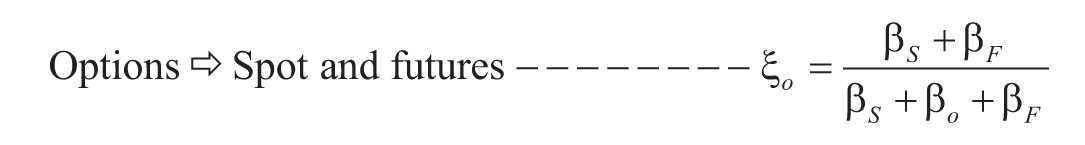
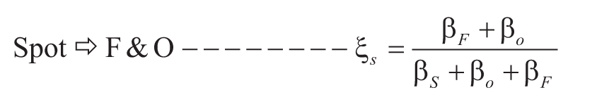
Equations (6), (7), and (8) gauge the relative contribution of futures, options, and spot markets, respectively. If the values of ξ_f, ξ_f or ξ_f is equal to 1, then it suggests its absolute dominance in terms of price discovery. We also evaluate the one-to-one analysis of these coefficients by applying equation (5) for respective markets. The results of both comparisons are discussed in the next section.

In measuring the volatility-based linkage, we run the threshold generalized autoregressive conditional heteroscedastic (TGARCH) model introduced by Zakoian (1994) under VECM framework and the dynamic conditional correlation generalized autoregressive conditional heteroscedastic (DCC-GARCH) model developed by Engle (2002). The rationale for applying TGARCH is associated with the time-varying characteristics of asset prices across markets. Numerous investigations also identified serial correlation in the volatility (Fama & French, 1988; Glosten et al., 1993; Just & Echaust, 2020; Karmakar, 2005; LeBaron, 1992), and as a result, the period of increased/decreased volatility follows a period of higher/lower volatility, thereby creating a kind of cluster of volatilities. This can be perfectly modeled via the GARCH model introduced by Bollerslev (1986). However, the clustering behavior of volatility is affected by the nature of the information released (i.e., positive/negative), which creates a varied magnitude of influence. The GARCH model is neutral to this effect and, hence, it cannot allow for stock volatilities’ asymmetric response to past returns. This phenomenon is well captured by the TGARCH model which adds a threshold parameter to accommodate for various degrees of volatility under different market conditions and measures how the three market responds to perceived positive and negative news. The general specification of the model is:

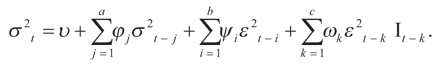
σ^{2}_{t} = υ + \sum_{j = 1}^{a} φ_{j} σ^{2}_{t - j} + \sum_{i = 1}^{b} ψ_{i} ε^{2}_{t - i} + \sum_{k = 1}^{c} ω_{k} ε^{2}_{t - k} I_{t - k} .

(9)

In equation (9), υ is the intercept term; σ²_{t – j} indicates the impact of previous period’s volatility and its persistency and its nature of impact on conditional variance (σ²_t ) is captured by φ_j. The effect of past shocks (ε²_{t – i}) on the current period’s volatility is revealed by the coefficient, ψ_i_. The last section of equation (5) highlights the asymmetric impact of new information on conditional volatility. In the last section, I_t _{– k} will have a value 1, if ε_t < 0 (bad information) and otherwise it will have the value 0. This clearly depicts that the TGARCH model will have a differential effect on the conditional volatility based on the nature of the information. If the information announced is in general good for the capital market, it will have an impact of only ψ_i on conditional variance, whereas if the information is negative or bad in nature, then the impact of new information will be amplified to ψ_{i +} ω_k. The results of the TGARCH model help us to ascertain the reaction of spot, F&O markets in terms of volatility when a piece of new information enters the market.

Theoretical understanding of cointegrated markets suggests that these markets exhibit a conditional correlation between themselves, and the nature of the correlation is assumed to be constant. Manera et al. (2006) opine that when a market is affected by innovations, the returns of the markets demonstrate dynamic interdependence in conditional volatility as well as in conditional correlation. Many studies examine the spillover effect between the spot and futures models using BEKK and other family of GARCH models (Kang et al., 2013; Karathanassis & Sogiakas, 2010; Karmakar, 2009; Mallikarjunappa & Afsal, 2010; Pati & Rajib, 2011; Tse, 1999). However, we do not find any empirical investigation which has examined the nature of conditional correlation among spot, futures, and options markets. We attempt to test the same using the multivariate dynamic conditional correlation generalized autoregressive conditional heteroscedastic (DCC-GARCH) model. The general specification of the DCC-GARCH model proposed by Engle (2002) is

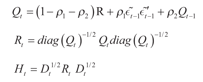
\begin{array}{l} Q_{t} = (1 - ρ_{1} - ρ_{2}) R + ρ_{1} {\int^{˜}}_{t - 1} {\int^{˜}}^{'}_{t - 1} + ρ_{2} Q_{t - 1} \\ R_{t} = d i a g {(Q_{t})}^{- 1 / 2} Q_{t} d i a g {(Q_{t})}^{- 1 / 2} \\ H_{t} = D_{t}^{1 / 2} R_{t} D_{t}^{1 / 2} \end{array}

(10)

In the above set of equations, R_t is the conditional quasi-correlation matrix that represents the dynamic conditional correlation between the variables and ρ₁ and ρ₂. These variables not only indicate the nature of conditional correlation but also control the conditional quasi-correlation dynamics. The values of ρ₁ and ρ₂ must be nonnegative, and the sum of these two parameters should be between 0 and 1. From the context of our study, ∈_t represents the residuals of the VECM-TGARCH model, H_t is the variance–covariance matrix of residuals, and D_t is a diagonal matrix of the GARCH coefficient. The value of the matrix Q_t is based on its own lag, standardized residuals of VECM ${\tilde{ϵ}}_{t - 1} = \frac{ϵ_{i, t}}{\sqrt{h_{i i, t}}}$

and the quasi-correlation matrix R (Bohl et al, 2011; Naoui et al., 2010). Engle (2002) suggests that under DCC-GARCH, the parameters to be estimated in the correlation process do not depend on the number of series which are required to be correlated and, hence, the DCC-GARCH model’s computational advantage is much higher than other classes of MGARCH models. This remark from the originator of the model justifies the utility of the DCC-GARCH model in this study. The result of DCC estimates not only helps us to infer about volatility interdependence (Frank & Hesse, 2009) but also adds to the literature on hedge ratio modeling and portfolio construction. The results of all these models are elucidated in the next section.

Results and Discussions

We first analyze the price-based interdependence to decipher the interdependence among spot and index derivatives. Here, we ascertain the short-run and long-run equilibrium relationship, direction of information flow and lead–lag relationship between spot and F&O markets. To examine the equilibrium relationship, first, we put the variables to the ADF test, the result of which is reported in Table 1. The results suggest that spot, futures, and options prices are not stationary at level as τ (tau) statistics are insignificant; however, they are significant at first difference which indicates that all the variables are of the integrated order 1.

Table 1.

ADF Test Result.

Variables	Null Hypothesis	Level Data		First Differenced Data
Variables	Null Hypothesis	τ Value	p value	τ value	p value
Spot price	i>H/i>₀: Nonstationary	−3.317385	0.0639	−32.26546	0.0000
Futures price		−3.212750	0.0823	−33.54001	0.0000
Options price		−2.734425	0.2227	–46.04168	0.0000
Residual		−11.43540	0.0000	—

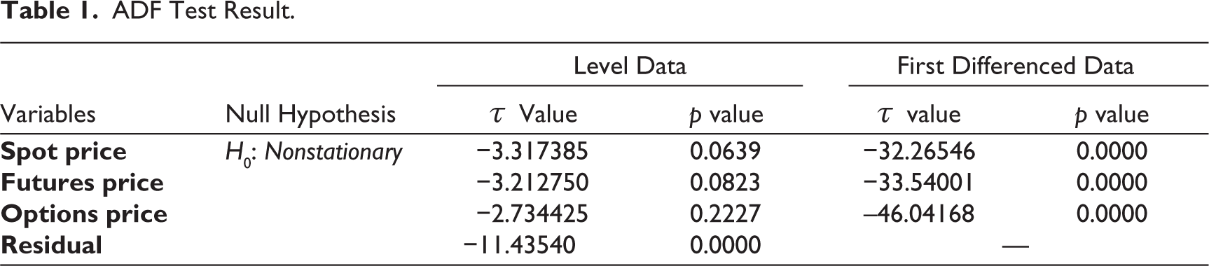
The ADF test statistics-based residual approach (Engle & Granger, 1987) suggest that there is a long-term comovement between options, futures, and spot, as price variables are of the order I(1) and their linear combination (i.e., residuals) is of the order I(0), i.e., stationary at level, during the study period. To further validate the evidence on the long-term cointegrating relationship among the variables, we run the Johansen cointegration test. To run this test and to use VECM system specification, we need to choose an optimal lag which is neither too small nor too large. This is because under-fitting of lags results in model misspecification and over-fitting makes the model more complex and less parsimonious (Enders, 2013). As the Johansen test is sensitive to the number of lags employed, we choose optimal lags based on the VAR lag selection approach, the result of which is depicted in Table 2. The approach reports five criteria with a maximum of eight lags for selecting the optimal lag that can be used in the Johansen test and VECM.

Table 2.

Lag Order Selection Criteria.

Lag	LR	FPE	AIC	SIC	HQ
0	NA	1.21e−10	−14.31786	−14.30537	−14.31316
1	10,874.35	1.71e−14	−23.18748	−23.13751	−23.16868
2	264.3519	1.40e−14	−23.38932	−23.30188*	−23.35642*
3	30.84572	1.38e−14*	−23.39999*	−23.27508	−23.35299
4	12.03998	1.39e−14	−23.39524	−23.23285	−23.33414
5	12.67986	1.39e−14	−23.39104	−23.19118	−23.31584
6	7.468483	1.40e−14	−23.38256	−23.14523	−23.29326
7	5.265169	1.42e−14	−23.37227	−23.09746	−23.26887
8	21.55238*	1.41e−14	−23.37553	−23.06324	−23.25803

Notes: *Lag order selected by the criterion.

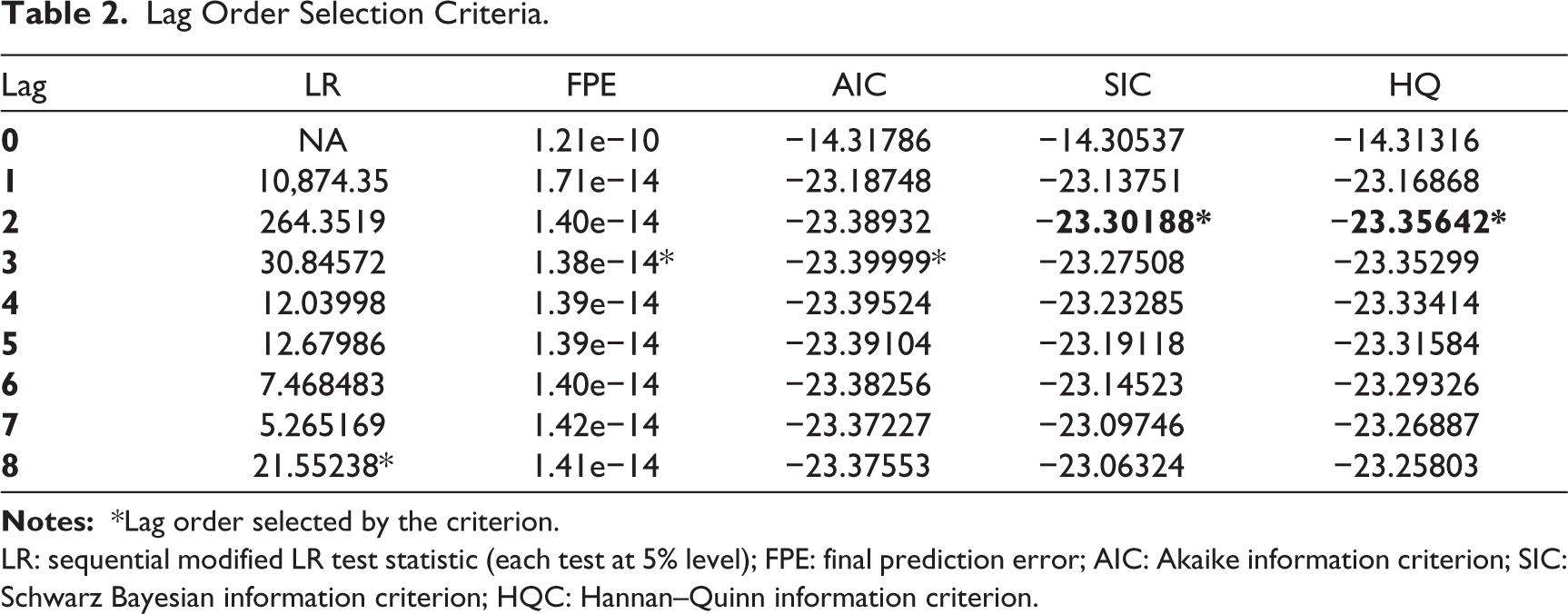
LR: sequential modified LR test statistic (each test at 5% level); FPE: final prediction error; AIC: Akaike information criterion; SIC: Schwarz Bayesian information criterion; HQC: Hannan–Quinn information criterion.

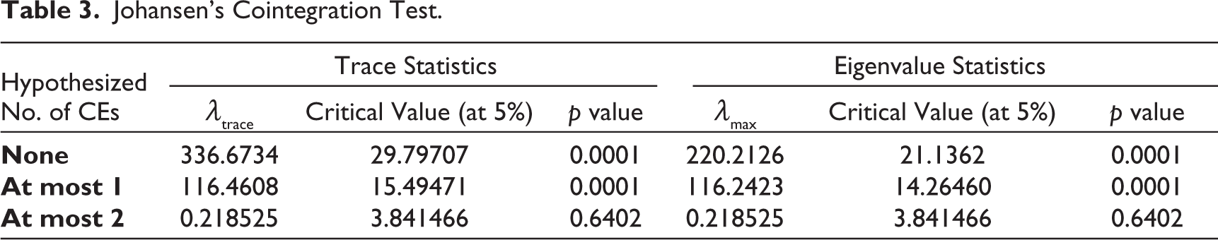
We select a lag of 2 as optimal on the basis of the Schwarz Bayesian and the Hannan–Quinn criterion, since SIC and HQC choose a lag which keeps the model more parsimonious by adding a penalty factor for higher lag selection (Gujarati, 2011). Then, we ran the Johansen test which upheld the existence of a long-run relationship between spot, F&O market. This finding is uniform in all the studies carried out in the past pertaining to spot–futures or spot–options cointegration. The results of the test are presented in Table 3. The cointegration test provides no evidence of the absence of cointegrating relationship among spot, futures, and options prices at the first null hypothesis since both the trace and eigenvalue statistics are significant at the 5% level.

Further, it does not reject the null hypothesis on the existence of at most two cointegrating equations during the study period as reported in Table 3. This suggests that spot, futures, and options prices have at least two cointegrating vectors and in general there may be information transmission between the markets. The test highlights the existence of a strong equilibrium relationship among these three markets, which is the first hint in deciphering the price interdependence. This implies that all three markets are characterized by efficiency in terms of pricing, and any discrepancy in this relation will create an arbitrage opportunity for the market players, which in turn align the price in the three markets.

Table 3.

Johansen’s Cointegration Test.

Hypothesized No. of CEs	Trace Statistics			Eigenvalue Statistics
Hypothesized No. of CEs	λ_trace	Critical Value (at 5%)	p value	λ_max	Critical Value (at 5%)	p value
None	336.6734	29.79707	0.0001	220.2126	21.1362	0.0001
At most 1	116.4608	15.49471	0.0001	116.2423	14.26460	0.0001
At most 2	0.218525	3.841466	0.6402	0.218525	3.841466	0.6402

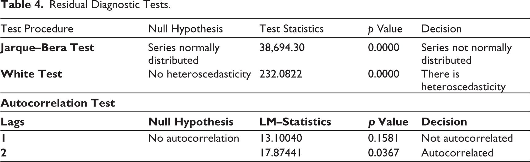
Though there is an equilibrium relationship among variables, we are not sure about the direction of relationship and which market reacts faster, what happens to the relationship in the short run? To verify the short-run and long-run dynamic relationship among the variables, we use VECM with a precondition of at least two cointegrating vectors as found under Johansen’s test. The initial test of VECM reports that the residuals of the model not only exhibit autocorrelation at second lag but also possess heteroscedastic variance as reported in Table 4. These two model specification problems can be resolved either using Newey–West’s heteroscedasticity and autocorrelation consistent standard error mechanism or using GARCH terms with maximum likelihood Marquardt estimation method. We modify our VECM with GARCH terms and run the VECM-TGARCH model, since our study is also oriented toward the identification of volatility-based asymmetric interdependence.

Table 4.

Residual Diagnostic Tests.

Test Procedure	Null Hypothesis	Test Statistics	p Value	Decision
Jarque–Bera Test	Series normally distributed	38,694.30	0.0000	Series not normally distributed
White Test	No heteroscedasticity	232.0822	0.0000	There is heteroscedasticity
Autocorrelation Test
Lags	Null Hypothesis	LM–Statistics	p Value	Decision
1	No autocorrelation	13.10040	0.1581	Not autocorrelated
2	No autocorrelation	17.87441	0.0367	Autocorrelated

The resultant VECM-TGARCH model with the ML–Marquardt estimation method reports the basic VECM parameters (i.e., speed of error correction and lagged variables) along with TGARCH coefficients. The results of VECM parameters for three system equations are provided in Table 5. The table reports two speed of adjustment terms relating to two cointegrating relations built into the specification so that it restricts the long-run behavior of the endogenous variables to converge to their cointegrating relationships while allowing for short-run adjustment dynamics (Bekhet & Yusop, 2009). However, the error corrective relationship among these variables is undefined and, hence, there is a necessity to interpret both the error correction terms. Though we find evidence for strong long-run cointegrating relations among the three markets, perhaps in the short run there will be deviations from the equilibrium level of spot price, futures price and option strike price due to internal and external market and economic factors. The speed of adjustment terms of VECM provide an indication of the ability of endogenous variable in adjusting these disequilibrium errors.

Table 5.

Price Linkage Measured via VECM.

Variables	Spot Market		Futures Market		Options Market
Variables	Coefficient	Probability	Coefficient	Probability	Coefficient	Probability
α	0.000125 (0.000306)	0.6833	0.000141 (0.000319)	0.6582	−0.00034 (0.000308)	0.2658
β ₁	0.082758 (0.147565)	0.5749	0.335012 (0.153999)	0.0296**	−0.08846 (0.092078)	0.3367
β ₂	−0.098974 (0.145011)	0.4949	−0.34003 (0.151314)	0.0246**	0.188782 (0.092903)	0.0422**
S ₁	−0.03553 (0.204684)	0.8622	0.124525 (0.214299)	0.5612	0.320148 (0.136695)	0.0192**
S ₂	−0.16695 (0.199692)	0.4031	−0.13204 (0.205459)	0.5205	−0.07967 (0.166117)	0.6315
F ₁	0.143629 (0.202294)	0.4777	−0.04723 (0.211883)	0.8236	−0.2961 (0.129787)	0.0225**
F ₂	0.156299 (0.192796)	0.4175	0.111517 (0.199415)	0.5760	0.057082 (0.170093)	0.7372
O ₁	−0.00101 (0.045711)	0.9823	0.014522 (0.048621)	0.7652	−0.16654 (0.055441)	0.0027***
O ₁	0.051326 (0.0437)	0.2402	0.053921 (0.047743)	0.2587	0.011178 (0.02912)	0.7011

Notes: *Significance at 10%; ** significance at 5%; *** significance at 1%.

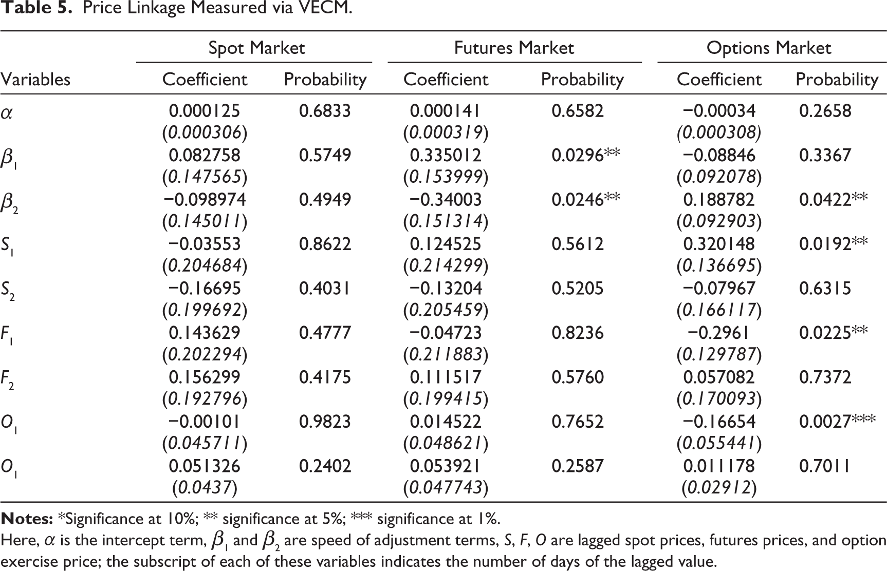
Here, α is the intercept term, β₁ and β₂ are speed of adjustment terms, S, F, O are lagged spot prices, futures prices, and option exercise price; the subscript of each of these variables indicates the number of days of the lagged value.

As per the results of VECM relating to spot equation, neither speed of adjustment terms (i.e., β₁ and β₂) of both cointegrating vectors nor the lagged price of spot, futures, and options have a significant impact on the spot prices. This evidence is contradictory to the theoretical understanding of the leading role played by F&O in a market setup. In the case of the futures equation, the first speed of adjustment term (i.e., β₁₎ does not provide strong evidence on long-run dynamics of futures since their values are positive and statistically insignificant, whereas in the case of the second error correction term (i.e., β₂), the futures prices correct the previous period’s deviation in price at a speed of almost 34% per day to arrive at convergence with the long-run equilibrium level. The insignificant spot, options, and futures lag in futures VECM specification leads us to infer about absence of information flow from the spot and options market to the futures market. Interestingly, in the case of options, β₁ coefficient contains a negative value with no statistical significance and β₂ coefficient, though significant has a positive sign. This suggests that the speed of adjustment term (β₂), instead of converging toward the equilibrium level, moves away from this level. This is a hint that the option market is not moving in the same direction as futures and spot markets. The divergence here may increase volatility in the options market and uncertainty for hedgers as ambiguity may prevail for some period about the market’s future direction. In contrast, the coefficients of lagged variables in the equation show that immediate previous-day price changes of spot, futures, and options have a highly significant impact on the current-day options strike prices. This is a sign about the information flow among these markets in the short run, in spite of the positive significant β_2, which indicates divergence in options prices from spot and future price levels in the long run.

In order to further validate the price interdependency among these markets, we run the BEVGC test along with the conventional pair-wise test. The one-to-one analysis of each of these market prices reported in Table 6 indicates that a unidirectional feedback relationship exists between the spot and options market as well as the F&O market; the reverse is not true since we do not find statistically significant evidence for the same under pair-wise test and the BEVGC test. Although we find significant evidence for unidirectional causality running from spot to futures as per the conventional pair-wise test, the same is absent in the case of the BEVGC test. Furthermore, the collective influence analysis carried out under the BEVGC test reports that there is no composite effect of spot and futures, F&O and options and spot on options, spot and futures market, respectively, since the ‘p’ values of BEVGC tests are insignificant.

Table 6.

Results of Feedback Relationship Test.

Dependent Market	Null Hypothesis	Pair-wise GC Test (F Statistic)	BEVGC Test ( Statistic)
One-to-one Influence
Spot	Futures doesn’t Granger cause spot	0.29411 (0.7452)	0.985051 (0.6111)
Spot	Options doesn’t Granger cause spot	2.08873 (0.1243)	2.520762 (0.2835)
Futures	Spot doesn’t Granger cause futures	3.98404** (0.0189)	1.294746 (0.5234)
Futures	Options doesn’t Granger cause futures	1.36722 (0.2552)	1.589922 (0.4516)
Options	Futures doesn’t Granger cause options	132.930*** (0.0000)	4.983239* (0.0828)
Options	Spot doesn’t Granger cause options	133.587*** (0.0000)	4.649708* (0.0978)
Collective Influence
Spot	F&O do not Granger cause spot		3.683785 (0.4505)
Futures	Spot and options do not Granger cause futures		2.955394 (0.5653)
Options	Spot and futures do not Granger cause options		5.450952 (0.2441)

Note: *Significance at 10%; **significance at 5%; ***significance at 1%.

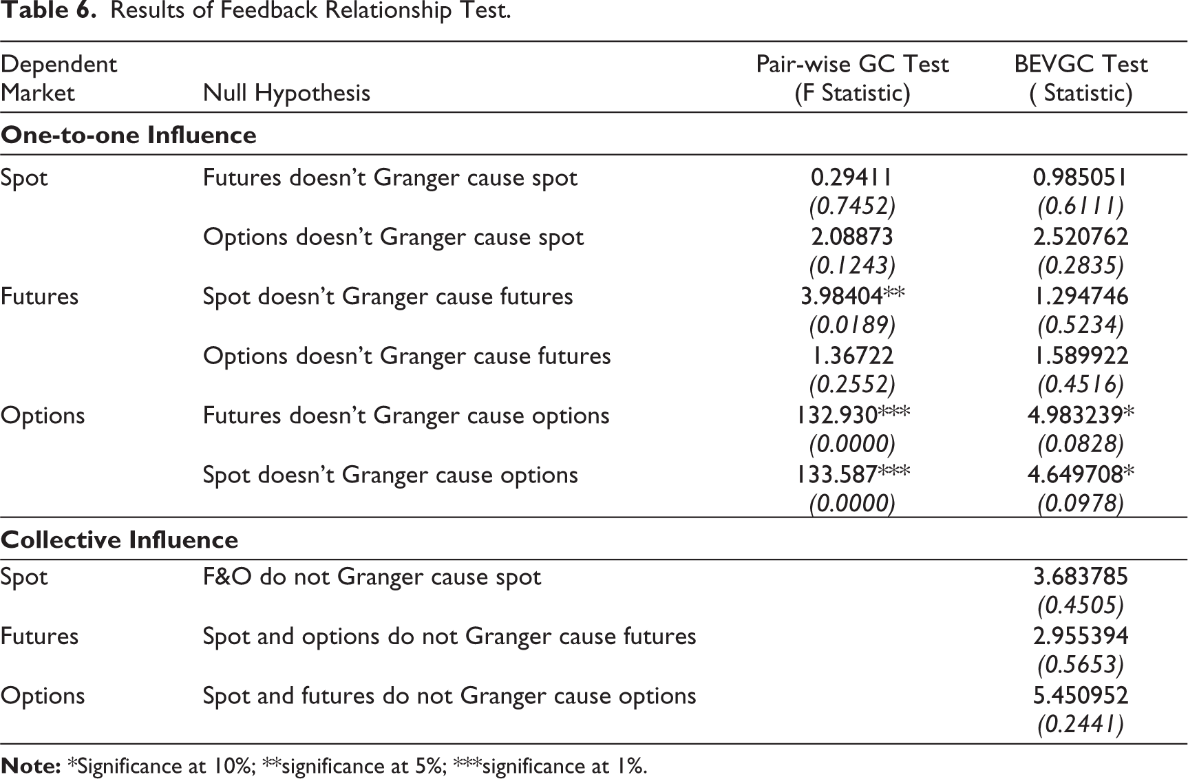
Thus, on the basis of the Granger causality test, we can infer that only the past values of spot and futures individually influence the current values in the options market. This is a confirmation that new information is first impounded in the spot and future market and then transmitted to the options market. Perhaps, we did not expect these findings because in general, the options market with comparatively lower transaction costs and higher leverage conditions against futures and spot should react first to any announcement or there should have been a feedback effect among these cointegrated markets. The above result further reinstates our earlier finding about options market inefficiency. This scenario can help non-hedgers to gain from market imperfection, whereas hedgers must cautiously monitor the changes to strategies for their entry–exit in the options market.

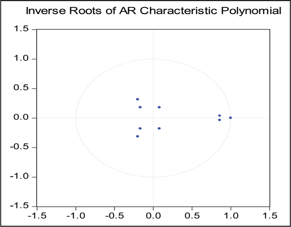
We verify the stability of VECM using the AR roots graph which plots the inverse roots of characteristic polynomials. The result of the VEC stability test is depicted in Figure 1. A stable process of VECM will have the modulus of root values less than one for the first root, as the companion matrix of a VECM with ‘k’ endogenous variables and ‘r’ cointegrating equations will have ‘k – r’ unit eigenvalues (Enders, 2013).

This study uses three variables, and the cointegration test confirms the existence of two cointegrating equations; hence, VECM-AR roots will have one root with the value of unity. Figure 1 also suggests that VEC specification imposes 1 unit root as we can see only one pointer is on the perimeter of the unit circle and, hence, the VECM used in the study is stable.

Figure 1.

VEC Stability Test.

In order to further prove the price interdependency among these markets, we use Schwartz and Szakmary’s factor weights to quantify relative contribution, which is on par with Hasbrouck’s information share approach and Gonzalo and Granger’s common factor weights (Theissen, 2002). We modify their approach to fit them to three market scenarios with simple (one-to-one) and composite (joint) comparisons. Table 7 portrays the relative contribution of each of these markets to long-run price interlinkage using Schwartz and Szakmary’s measure to figure out which market has a greater influence on price discovery and in turn suggests the long-run leading role played by a market. This can happen in a significant manner if any of the PD₁ or PD₂ coefficients are equal to 1.

Table 7.

Relative Price Discovery Contribution Measure.

PD Direction	PD₀₁	PD₀₂
Futures ⇨ Spot	0.1981	0.2255
Options ⇨ Spot	0.4833	0.3440
Options ⇨ Futures	0.7911	0.6430
Futures ⇨ Spot and options	0.3342	0.4584
Options ⇨ Spot and futures	0.8253	0.6993
Spot ⇨ F&O	0.8365	0.8423

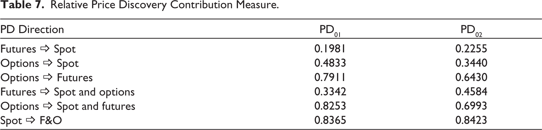
The direct comparison of the spot, futures, and options market with one another suggests none of the markets enjoys absolute dominance in playing a price discovery role as the Schwarz and Szakmary’s factor weights in both cointegrating equation is not equal to 1. The low factor weights of futures on spot indicate the superiority of the spot market in performing the price discovery function. The comparison of options to spot indicates no leading role played by either of the markets. However, options play a slightly dominant role against futures in performing the price discovery function.

We also check whether the interactiveness of the dual market will have a bearing on the price discovery function of the other market. The factor weights of futures which are computed using the other two market speed of adjustment terms do not provide evidence on the leading role played by futures. Similar to the results of one-to-one factor weights, we further discover proof for spot and options markets’ significant role in price discovery. Altogether, it is evident that in the backdrop of two cointegrating relationships (PD₁ and PD₂), perhaps the spot market’s role appears to be dominant as the price discovery measures are higher compared to options and futures. This finding is consistent with findings of the studies carried from an Indian market perspective (Babu & Srinivasan, 2014; Ekta, 2013; Misra et al., 2006; Pandey, 2014; Pathak et al., 2014) with only spot–futures comparison. All these results and findings help us to infer that there is strong price-based interlinkage among spot, futures, and options markets.

We next account for possible volatility-based interdependence among the three markets using GARCH family models. The volatility-based approach targets how the three markets react to positive and negative innovations (shocks) and what sort of conditional correlation the markets share among each other. We first verify whether volatility in one market is affected by price changes in the other markets and, if so, whether its effect is asymmetric in nature. For this purpose, we use the TGARCH model proposed by Zakoian (1994), the result of which is described in Table 8. The coefficient c is a constant term in the TGARCH equation, φ reveals the influence of past innovations on conditional volatility in spot, futures, and options price change, ψ indicates the effect of previous days’ volatility on conditional volatility and asymmetric effect of new information is captured by ω.

Table 8.

Volatility Interlinkages.

Variables	Spot Market		Futures Market		Options Market
Variables	Coefficient	Probability	Coefficient	Probability	Coefficient	Probability
c	0.00000365	0.0001	0.00000405	0.0000	0.0000406	0.0000
ϕ	0.008831	0.1977	0.010305	0.1550	0.515745	0.0000
ψ	0.943747	0.0000	0.9416	0.0000	−0.06979	0.0331
ω	0.02375	0.0043	0.022759	0.0074	−0.28424	0.0052
DCC–Quasi-correlation
	Spot		Futures		Options
Spot	———		0.9998197 (0.0000)		0.9843673 (0.0000)
Futures	0.9998197 (0.0000)		———		0.983586 (0.0000)
Options	0.9843673 (0.0000)		0.983586 (0.0000)		———
DCC Adjustment Terms
ρ ₁	0.599492 (0.0000)		ρ ₂		0.0872257 (0.0370)

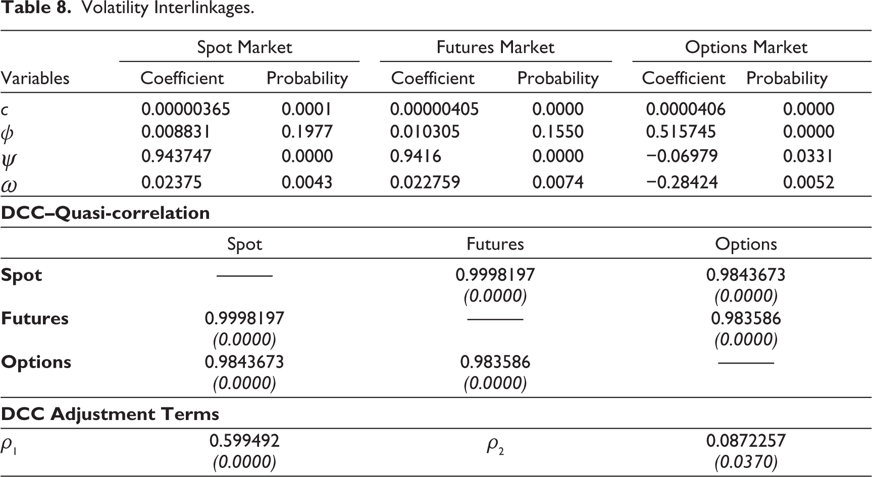
It is clear from the results of the TGARCH model that only volatility in the options market is significantly influenced by past innovations in options strike price change; however, in the case of volatility clustering, all three markets share similar characteristics. The result further establishes our earlier finding of options inefficiency and the opportunities it offers. The statistically significant ψ coefficient in spot, futures, and options is an indication that the past behavior of volatility has a persistent effect on the current period’s volatility in the three markets during the period of study. The highly significant and positive asymmetry coefficient denoted by ω in spot and futures returns points out that negative news exerts a significant impact on the price fluctuations in the spot and futures market. The value of ψ coefficient indicates that negative return shocks will increase the volatility in the spot market by 2.38% and 2.28% more than positive return shocks of similar scale. However, in the case of options, though ω is significant its value is negative, which is an indication that during the study period leverage effect, generally exhibited by options return volatility, is absent. These findings also have implications for investors, portfolio managers, and corporates to incorporate time-variant and persistence volatility in their risk management model, since abrupt spikes in volatility may result in sizable losses.

Besides modeling conditional volatility, we also account for conditional covariance using DCC-GARCH proposed by Engle (2002), which assumes a conditional correlation between the variables vary over time. In this study, conditional means of price change are modeled as a restricted VAR process. On the other hand, conditional covariance follows the MGARCH-DCC process with the GARCH (1,1) process of variance of each disturbance term. The dynamic conditional correlation in the context of our study describes a highly significant conditional quasi-correlation among spot, F&O market volatility as presented in Table 8. This reveals that there is comovement of asset prices in these three markets. The adjustment terms (i.e., ρ₁ and ρ₂) not only satisfies the nonnegativity condition and their sum is less than unity, but also they are statistically significant. This is an indication that the conditional correlation among standardized residuals of spot, futures, and options are time variant. This finding can be utilized in altering the traditional constant hedge ratio which assumes the correlation between the two markets are time invariant (Bauwens et al., 2006). In total, the results found via the analysis of the price and volatility relationship among spot, futures, and options is an indication of the time-dependent interdependence among these markets.

Concluding Remarks

This study is focused on analyzing the interdependence among the Nifty50 index, Nifty50 futures, and Nifty50 options in the context of price and volatility-based association. There are studies carried out in both the emerging and the matured markets which examined the interdependence between spot and derivatives in the context of information efficiency, price discovery, volatility spillover, and stabilizer role. However, these studies are largely bimarket in nature, except for the study of Fleming et al (1996) and Jong and Donders (1998) who analyzed all three markets using trading costs data. Through our detailed review of empirical literature, we find a void in terms of the studies which measure the collective influence of spot, F&O on the price and volatility relationship. We considered this gap in the literature and made an attempt to analyze the same from the Indian perspective using the benchmark index, Nifty50.

We infer the price-based relation among the three markets in the light of the market’s ability to lead other cointegrated markets, the nature of influence of past prices quoted in these markets and on the basis of the feedback relationship. The findings on these aspects advocate the stronger leading role played by spot against F&O, the significant positive (negative) influence of the previous day’s spot (futures) price change on options’ price change and unidirectional VEC Granger causality running from spot and futures to options market. The main reason that can be attributed to these results is the market microstructure innovations introduced in the form of call-auction mechanism in the spot market, increased preference of market participant toward Nifty50 index-based products made the index more liquid and reduced popularity of index futures among Indian stock derivatives market players post global crises period.

Our inquiry in ascertaining the reaction of spot, futures, and options market to shocks which are caused by positive and negative news indicate that the volatility in spot and futures market are significantly influenced by negative returns and such evidence is not found in the case of options volatility. We also find that the past behavior of volatility has a persistent effect on the current period’s volatility in all three markets. However, the effect of past shocks on conditional volatility is stronger only in the case of options with comparatively lower volatility persistency factor. We further explore the existence of conditional correlation to assess the extent and nature of association among these interlinked markets. The results of dynamic conditional correlation among standardized residuals of spot, futures, and options confirm stronger time-varying volatility interlinkage among these markets, and in the event of any crisis or significant shocks caused by negative returns, the correlation among these markets will increase significantly (Mikkonen, 2017).

The study finding of time-varying conditional correlation can enable the researchers, portfolio managers, and corporates to implement time-varying nature of conditional correlation into hedge ratio construction instead of assuming a constant correlation between the markets. Traders can rely on technical tools to recognize volatility trends and modify their trading strategies. The regulatory bodies and bourses must deploy measures to enhance liquidity and promote market integrity and efficiency to avoid increased divergence of sentiment. The findings also imply that the theoretical argument of F&O leading the spot market may not always hold good and in fact, these markets exhibit a price and volatility-based association among themselves temporally.

Footnotes

Declaration of Conflicting Interests

The authors declared no potential conflicts of interest with respect to the research, authorship and/or publication of this article.

Funding

The authors received no financial support for the research, authorship and/or publication of this article.

References

Abhyankar

A. H.

(1995). Return and volatility dynamics in the FTSE 100 stock index and stock index futures market. The Journal of Futures Market, 15(4), 457−488.

Augustin

, Brenner

, & Subrahmanyam

M. G.

(2018). Informed options trading prior to M&A announcements: Insider trading? Management Science, 1–24.

Avinash, & Mallikarjunappa

(2017). Impact of economic crises on the price discovery dynamics of spot & index futures market. Asian Journal of Research in Banking and Finance, 7(7), 78–88. 10.5958/2249-7323.2017.00070.0

Babu

, & Srinivasan

(2014, March). Testing the co-integration in Indian commodity markets: A study with reference to Multy Commodity Exchange India Ltd. Indian Journal of Finance, 8(3), 35−43.

Bandivadekar

, & Ghosh

(2003). Derivatives and volatility on Indian Stock markets. Reserve Bank of India Occasional Papers, 24(3), 187–201.

Bauwens

, Laurent

, & Rombouts

J. V.

(2006). Multivariate GARCH models: A survey. Journal of Applied Econometrics, 21, 79–109.

Bekhet

H. A.

, & Yusop

N. Y.

(2009). Assessing the relationship between oil prices, energy consumption and macroeconomic performance in Malaysia: Cointegration and vector error correction model (VECM) approach. International Business Research, 2(3), 152–175.

Bhattacharya

(1987). Price changes of related securities: The case of call options and stocks. Journal of Financial & Quantitative Analysis, 22(1), 1–15.

Bhuyan

, & Chaudhury

(2005). Trading on the information content of open interest: Evidence from the US equity options market. Derivatives Use, Trading & Regulation, 11(1), 16–36.

10.

Black

(1975). Fact and fantasy in use of options. Financial Analysts Journal, 31, 36–41.

11.

Bodhla

B. S.

, & Jindal

(2008). Equity derivatives in India: Growth pattern and trading volume effects. The ICFAI Journal of Derivatives Market, 5(1), 62–82.

12.

Bohl

M. T.

, Salm

C. A.

, & Schuppli

(2011). Price discovery and investor structure in stock index futures. The Journal of Futures Market, 31(3), 282–306.

13.

Bollerslev

(1986). Generalized autoregressive conditional heteroskedasticity. Journal of Econometrics, 31(3), 307–327. 10.1016/0304-4076(86)90063-1

14.

Boyle

P. P.

, Byoun

, & Park

H. Y.

(2002). The lead–lag relation between spot and option markets and implied volatility in options prices. Research in Finance, 19, 269–284.

15.

Brooks

, Rew

A. G.

, & Ritson

(2001). A trading strategy based on the lead–lag relationship between the spot index and futures contract for the FTSE 100. International Journal of Forecasting, 17(1), 31–44.

16.

Chakravarty

, Gulen

, & Mayhew

(2004). Informed trading in stock and options market. The Journal of Finance, 59, 1235–1257. 10.1111/j.1540-6261.2004.00661.x

17.

Chan

, Chung

Y. P.

, & Fong

W.-M.

(2002). The informational role of stock and option volume. The Review of Financial Studies, 15(4), 1049–1075.

18.

Choudhary

, & Bajaj

(2013). Price discovery process in Nifty50 spot and futures market. Global Business Review, 14(1), 55–88.

19.

Cremers

, Fodor

, & Weinbaum

(2015). Where do informed traders trade first? Options trading activity, news releases, and stock return predictability.

20.

Debasish

S. S.

(2009). Effect of futures trading on spot-price volatility: Evidence for NSE Nifty50 using GARCH. The Journal of Risk Finance, 10(1), 67–77. 10.1108/15265940910924508

21.

Dimitriou

, Kenourgios

, & Simos

(2013). Global financial crisis and emerging stock market contagion: A multivariate FIAPARCH–DCC approach. International Review of Financial Analysis, 30, 46-56.

22.

Easley

, O’Hara

, & Srinivas

P. S.

(1998). Option volume and stock prices: Evidence on where informed traders trade. The Journal of Finance, 53(2), 431–465.

23.

Ekta. (2013). Lead lag relationship between futures and spot market: Empirical evidence from Bank Nifty50. Global Research Analysis, 2(12), 162–163.

24.

Enders

(2013). Applied econometric timeseries (3rd ed.). Wiley India Pvt Ltd.

25.

Engle

(2002). Dynamic conditional correlation: A simple class of multivariate generalized autoregressive conditional heteroskedasticity models. Journal of Business & Economic Statistics, 20(3), 339–350. https://www.jstor.org/stable/pdf/1392121.pdf

26.

Engle

R. F.

, & Granger

W. J.

(1987). Cointegration and error correction: Representation, estimation, and testing. Econometrica, 55(2), 251–276.

27.

Fama

E. F.

, & French

K. R.

(1988). Permanent and temporary components of stock prices. Journal of Political Economy, 96(2), 246–273.

28.

Fleming

, Ostdeik

, & Whaley

R. E.

(1996). Trading costs and the relative rates of price discovery in stock, futures, and options markets. The Journal of Futures Market, 16(4), 353–387.

29.

Frank

, & Hesse

(2009). Financial spillovers to emerging markets during the global financial crisis. IMF Working Paper-WP/09/104, 1–20. https://www.imf.org/en/Publications/WP/Issues/2016/12/31/Financial-Spillovers-to-Emerging-Markets-During-the-Global-Financial-Crisis-22936

30.

Frino

, & West

(2002). The lead–lag relationship between stock indices and stock index futures contracts: Further Australian evidence. ABACUS, 35(3), 333–341.

31.

Futures Industry Association. (2022). Global futures and options trading hits another record in 2021. https://www.fia.org/fia/articles/global-futures-and-options-trading-hits-another-record-2021

32.

Glosten

L. R.

, Jagannathan

, & Runkle

D. E.

(1993). On the relation between the expected value and the volatility of the nominal excess return on stocks. The Journal of Finance, 48(5), 1779–1801.

33.

Gujarati

(2011). Econometrics by example (1st ed.). Palgrave Macmillan.

34.

Holowczak

, Simaan

Y. E.

, & Wu

(2006). Price discovery in the U.S. stock and stock options markets: A portfolio approach. Review of Derivatives Research, 9, 37–65. BIBLIOGRAPHY \l 1033

35.

IMF. (2021). World economic outlook. https://www.imf.org/en/Publications/WEO/Issues/2021/03/23/world-economic-outlook-april-2021

36.

Jong

F. D.

, & Donders

M. W.

(1998). Intraday lead–lag relationship between the futures, options and stock market. European Finance Review, 1(3), 337–359. http://rof.oxfordjournals.org/content/1/3/337.full.pdf+html

37.

Just

, & Echaust

(2020). Stock market returns, volatility, correlation and liquidity during the COVID-19 crisis: Evidence from the Markov switching approach. Finance Research Letters, 37. 10.1016/j.frl.2020.101775

38.

Kakati

R. P.

, & Kakati

(2007). Impact of futures and options trading on index stocks’ systematic risk, correlation structure and volatility. The ICFAI Journal of Applied Finance, 13(8), 5–19.

39.

Kang

S. H.

, Cheong

, & Yoon

S. M.

(2013). Intraday volatility spillovers between spot and futures indices: Evidence from the Korean stock market. Physica A: Statistical Mechanics and its Applications, 392(8), 1795–1802.

40.

Karathanassis

, & Sogiakas

(2010). Spillover effects of futures contracts initiation on the cash market: A regime shift approach. Review of Quantitative Finance and Accounting, 34(1), 95–143.

41.

Karmakar

(2005). Modeling conditional volatility of the Indian stock markets. VIKALPA, 30(3), 21–37. 10.1177/0256090920050303

42.

Karmakar

(2009). Price discoveries and volatility spillovers in S&P CNX Nifty50 futures and its underlying index CNX Nifty50. Vikalpa: The Journal for Decision Makers, 34(2), 41–56.

43.

Kawaller

I. G.

, Koch

P. D.

, & Koch

T. W.

(1987). The temporal price Relationship Between S&P 500 futures and the S&P 500 Index. The Journal of Finance, 42(5), 1309–1329. http://www.jstor.org/stable/2328529.

44.

LeBaron

(1992). Some relations between volatility and serial correlations in stock market returns. The Journal of Business, 65(2), 199–219. http://www.jstor.org/stable/2353162

45.

Mahajan

, & Singh

(2012). Return, volume and volatility relationship in the Indian stock market: A pre- and post futures analysis. Finance India, 26(1), 163–186.

46.

Mallikarjunappa

, & Afsal

E. M.

(2010). Price discovery process and volatility spillover in spot and futures markets: Evidences of individual stocks. Vikalpa: The Journal for Decision Makers, 35(2), 49–62.

47.

Manaster

, & Rendleman

R. J.

(1982). Option prices as predictors of equilibrium stock prices. The Journal of Finance, 37(4), 1043–1057.

48.

Manera

, McAleer

, & Grasso

(2006). Modelling dynamic conditional correlations in the volatility of spot and forward oil price returns. Applied Financial Economics, 16(7), 525–533.

49.

Mikkonen

(2017). Time-varying conditional correlation: Effect on international portfolio diversification in Southeast Asia. University of Jyväskylä, School of Business and Economics. University of Jyväskylä. https://jyx.jyu.fi/dspace/bitstream/handle/123456789/52762

50.

Misra

, Kannan

, & Misra

S. D.

(2006). Arbitrage opportunities in the futures market: A study of NSE Nifty50 Futures. Proceedings of 8th Global Conference of Actuaries (pp. 401–411). GCA. https://www.actuariesindia.org/downloads/gcadata/8thGCA/Arbitrage%20Opportunities%20in%20the%20Indian%20Future%20M.PDF

51.

Mukherjee

, & Mishra

R. K.

(2006). Lead–lag relationship between equities and stock index futures market and its variation around information release: Empirical evidence from India. NSE Working Paper 39. http://nseindia.com/content/research/comppaper155.pdf

52.

Naoui

, Liouane

, & Brahim

(2010). A dynamic conditional correlation analysis of financial contagion: The case of the subprime credit crisis. International Journal of Economics and Finance, 2(3), 85–96. ccsenet.org/journal/index.php/ijef/article/download/5922/5341

53.

National Stock Exchange India Ltd (NSE). (2015). NSE Newsletter (progress of futures and options market). NSEindia.com: http://www.nseidia.com/research/dynaContent/nsenewsletter.htm

54.

NSE. (2016). NSE makes India proud. NSE Press Release. Mumbai: NSE. https://www.nseindia.com/content/press/PR_cc_12052016.pdf

55.

S. X.

, Pan

, & Poteshman

A. M.

(2008). Volatility information trading in the option market. The Journal of Finance, 63(3), 1059–1091.

56.

Ota

(2003). The impact of price and return models on value relevance studies: A review of theory and evidence. Accounting Research Journal, 16(1), 6–20.

57.

Padhi

P. K.

(2015). Derivative trading in Indian capital market: An empirical study of NSE. Pacific Business Review International, 8(2), 89–94.

58.

Pan

, & Poteshman

(2006). The information in option volume for future stock prices. Review of Financial Studies, 19, 871–908.

59.

Pandey

(2014). Price discovery and volatility spill over in spot and futures: An empirical study of gold market in India. Tactful Management Research Journal, 2(10), 1–5.

60.

Pathak

R. Ranajee

, & Kumar

(2014). Price discovery in the equity derivatives market: A literature survey. Indian Journal of Finance, 8(6), 47–57.

61.

Pati

P. C.

, & Rajib

(2011). Intraday return dynamics and volatility spillovers between NSE S&P CNX Nifty50 stock index and stock index futures. Applied Economics Letters, 18(6), 567–574. http://www.tandfonline.com/doi/pdf/10.1080/13504851003742442?needAccess=true

62.

Rajput

, Kakkar

, Batra

, & Gupta

(2012). Price discovery in Indian stock market: The case of S&P CNX Nifty50 index. Investment Management and Financial Innovations, 9(3), 120–129.

63.

Rastogi

, Reddy

V. N.

, & Kotha

K. K.

(2014). Order imbalance and returns: Evidence of lead–lag relationship. The IUP Journal of Financial Risk Management, 11(2), 34–48.

64.

Sarangi

S. P.

, & Patnaik

U. S.

(2007). A study on the impact of futures and options on spot market volatility: A case of S&P CNX Nifty50 index. The ICFAI Journal of Applied Finance, 13(4), 58–72.

65.

Schwarz

T. V.

, & Szakmary

A. C.

(1994). Price discovery in petroleum markets: Arbitrage, cointegration, and the time interval of analysis. The Journal of Futures Market, 14(2) 147–167.

66.

Sehgal

, & Kumar

V. N.

(2007). The relationship between stock market variables and option market liquidity: Evidence from India. The ICFAI Journal of Derivatives Market, 4(3), 7–25.

67.

Srivastava

, Yadav

S. S.

, & Jain

P. K.

(2007). Effect of derivative security on volatility: A study in the context of Indian stock market. Finance India, 21(4), 1271–1296.

68.

Stoll

H. R.

, & Whaley

R. E.

(1990). The dynamics of stock index and stock index futures returns. The Journal of Financial and Quantitative Analysis, 25(4), 441–468. http://www.jstor.org/stable/2331010

69.

Theissen

(2002). Price discovery in floor and screen trading system. Journal of Empirical Finance, 9(4), 455–474. 10.1016/S0927-5398(02)00005-1

70.

Thenmozhi

(2002). Futures trading, information and spot price volatility of NSE-50 index futures contract. NSE Working Paper. https://www.nseindia.com/content/research/Paper59.pdf

71.

Tse

(1999). Price discovery and volatility spillovers in the DJIA index and futures markets. The Journal of Futures Market, 19(8), 911–930. 10.1002/(SICI)1096-9934(199912)19:8<911::AID-FUT4>3.0.CO;2-Q

72.

Zakoian

J. M.

(1994). Threshold heteroskedastic models. Journal of Economic Dynamics and Control, 18(5), 931–955. http://www.sciencedirect.com/science/article/pii/0165188994900396

Do Spot,Futures,and Options Markets Exhibit Price and Volatility Interdependence? Evidence from India