Recent Developments in DSGE Modelling: Beyond FIRE

Abstract

This survey focuses on the standard assumption in DSGE models: rational expectations (RE) with perfect information (PI) aka full information (FI)—hence FIRE. RE means model consistent expectations—agents be they households, firms, banks or policymakers know your model. PI (or FI) means agents observe or can infer the current and past state variables in your model. RE + PI (or FIRE) is a strong assumption. The purpose of this survey is to examine the literature that relaxes RE or PI or both. This is relevant for DSGE models in general, but particularly so for the efficacy of monetary policy in a New Keynesian environment when the expectation by agents of future policy is of crucial importance.

JEL Classification: C11, C18, C32, E32

Introduction

There have been a number of recent assessments of the ‘state of macro’ and the con­tribution of dynamic stochastic general equilibrium (DSGE) models—a list that is by no means exhaustive would include: Blanchard (2009, 2016), Blanchard et al. (2010, 2013), Driffill (2011), Pesaran and Smith (2011), Blanchard and Summers (2017), Vines and Wils (2018), Christiano et al. (2018) and Levine (2020).

This survey has a more narrow focus on the standard assumption in DSGE models: rational expectations (RE) with perfect information (PI) aka full information (FI)—hence FIRE. RE means model-consistent expectations—agents be they households, firms, banks or policymakers know your model. PI (or FI) means agents observe or can infer the current and past state variables in your model. RE + PI (or FIRE) is a strong assumption. The purpose of this survey is to examine the literature that relaxes RE or PI or both. This is relevant for DSGE models in general, but particularly so for the efficacy of monetary policy in a New Keynesian (NK) environment when the expectation by agents of future policy is of crucial importance.

We begin with departures from RE and a recent behavioural macroeconomics litera­ture. The ‘Behavioural Macro models’ section sets out the most common equilibrium concepts found in this literature. The third section sets out a standard NK model we use as an application in the rest of the paper. The fourth section moves on to models with heterogeneous agents consisting of both RE and non-RE agents and examines a class of equilibria when the latter can learn from the former through reinforcement learning. The fifth section then moves on to RE models where the PI assumption is relaxed in favour of imperfect information (II). The sixth section reviews important empirical results that assess, first, what we describe as the ‘wilderness’ of departures from RE and, second, the ability of the RE NK model with the II assumption to provide a better data fit than PI. The seventh section concludes the article.

Beyond RE: Equilibrium Concepts

In departures from RE, two sets of equilibrium concepts and related literature need distin­guishing. The first is statistical learning, which poses the question: Can agents learn to be rational through econometrics and, in particular, recursive least-squares learning? The second are a class of equilibria which do not converge to RE which we term behavioural macro-models. We consider these in turn.

Statistical Learning

Applications to macroeconomics were pioneered by Evans and Honkapohja (2001). The main idea is to replace RE with statistical forecasts based on knowledge of the structure of the RE solution—perceived law of motion (PLM) found by recursive least squares. A statistical equilibrium is then one where in a stochastic steady state the PLM is equal to the actual law of motion (ALM). If the learning processes n converge in this sense and the PLM = ALM = the RE equilibrium, we have what the literature terms E-Stability . This idea has been described as the ‘principle of cognitive’ consistency: ‘economic agents should be as smart as (good) economists’ (see the survey by Evans & Honkapohja, 2009). Other more recent surveys on statistical learning that their seminal contribution subsequently produced include Milani (2012) and Eusepi and Preston (2018). It should be noted that these papers adopt different approaches to learning—Euler learning versus an­ticipated utility discussed later and see also section 4.4 of Eusepi and Preston (2016). But either approach assumes agents are good econometricians and use well-specified forecasts of the model RE equilibrium.

To formalize the concept, consider the state-space form of a log- linearized DSGE model:

$A_0{y}_{t-\text{1}}\text{ + }{A}_{\text{1}}{y}_t\text{+ }{A}_{\text{2}}{E}_t{y}_{t+1}\text{ + }{B}_{\text{0}}{w}_t\text{ = 0,}$

(1)

where y_t is the state vector of endogenous variables in deviation form about a steady state. Matrices are functions of parameters j. The model is driven by exogenous driving AR(1) processes w_t.

$w_{t+\text{1}}\text{ = }{\rho }_w{w}_t\text{+ }{\in }_{t+1}{\in }_t\sim i.i.d.$

The minimal state variable (MSV) RE solution is

$y_t=b{y}_{t-1}\text{+ }c{w}_t.$

(2)

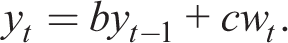
In the OLS learning equilibrium, agents know the form of the solution (2) and use recur­sive least squares to estimate

$y_t=b_t{y}_{t-1}\text{+ }{c}_t{w}_t,$

(3)

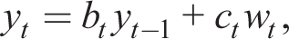
where [b_t, c_t] are time-varying parameters. E-stability has a large literature in itself, which includes McCallum (2007) and Ellison and Pearlman (2011).

Behavioural Macro-models

This class of models have one or more of the following features: (a) adaptive expectations in models of individual rationality (b) heterogeneous expectations and reinforcement learning (c) cognitive discounting and (d) agent inattention in otherwise rational mod­els. We examine five concepts in turn.

Concept I: Restricted Perception Equilibria (RPE): In an RPE, agents misspecify the law of motion (2). For example, they may not observe w_t and assume a first-order VAR

$y_t=b_t{y}_{t-1}\text{+}{\in }_t\text{}\text{},$

(4)

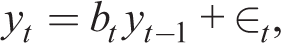
Let y_i,t be the ith component of y_t. Then assuming y_t is observable (the data). Assume a perceived law of motion in the form of simple AR(1) learning rules

$y_{i\text{},}{}_t={\rho }_i{y}_{i,t-1}\text{+}{\in }_{i\text{},}{}_t,$

(5)

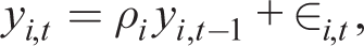
Solving for the actual law of motion, this leads to first-order autocorrelations in the stochastic steady state F (ρ, j), where ρ is the row vector of ρ_i and j are remaining parameters. Then given j, the stochastic consistent expectations equilibrium (SCEE) is the solution with the fixed point:

$\rho *=F(\rho *,\vartheta )\Rightarrow \rho *=\rho *(\vartheta ).$

(6)

See Hommes and Zhu (2014) and Hommes et al. (2023). It should be stressed that the SCEE is not the RE equilibrium, unlike statistical learning with e-stability.

Gobbi and Grazzini (2015) perform OLS on a first-order VAR of the full state, includ­ing shock processes. Eusepi and Preston (2011) perform OLS on a finite approximation of an infinite VAR of a subset of the state space. Hommes and Zhu (2015) use a parsi­monious first-order VAR to fit mean and persistence of each state variable to data. All these papers assume the solution of an RE model can be approximately expressed as a finite VAR, which in itself can be a strong assumption as shown by Fernandez-Villaverde et al. (2007). All these papers also use the SCEE concept (aka a Bayesian learning equilibrium). This contrasts with k-level thinking of Garcia-Schmidt and Woodford (2019) and Farhi and Werning (2019), where beliefs are updated iteratively with observed temporary and non-stochastic expectations equilibria over n stages.

Concept II: k-Level Thinking: See Garcia-Schmidt and Woodford (2019) and Farhi and Werning (2019). Consider a consumption function (derived later) where consumption (C_t) of a household is a function of the expected present and future interest rate and factor prices (the wage and profits). Write as

$C_t=f\left(X_t,E\left[X_{t+1},X_{t+2},\mathrm{..}\right]\right).$

(7)

with perfect foresight E[X_{t + i}] = X_{t + i}, so beliefs coincide with outcomes. In a stochas­tic environment, they coincide on average. k-level with k = 1 thinking proposes a temporary equilibrium such that given a set of beliefs ${\widehat{X}}_{t+i}^0$ which can be an initial RE equilibrium or steady state, then given observations of X_t

$C_t^1=f\left(X_t,{\stackrel{⌢}{X}}^0{}_{t+1},{\stackrel{⌢}{X}}^0{}_{t+2}\mathrm{..}\right).$

(8)

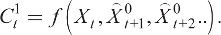
Similarly, for k = 2 thinking, we have

$C_t^2=f\left(X_t,{\stackrel{⌢}{X}}^1{}_{t+1},{\stackrel{⌢}{X}}^1{}_{t+2}\mathrm{..}\right).$

(9)

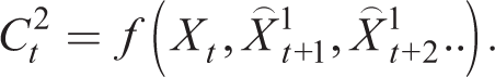
and so on. In the applications of this concept cited, as k → ∞, this iterative process converges with the RE equilibrium and has also been used to compute the solution of RE models.

Concept III: Adaptive Expectations: Adaptive expectations (AE) has a long his­tory in macroeconomics going back to Milton Friedman; see Friedman (1968). The AE rule takes the form:

$E_t^{*}{y}_{t+1}=E_{t-1}^{*}{y}_t+\lambda \left(y_t-E_{t-1}^{*}{y}_t\right);\lambda \in \left[0,1\right].$

(10)

By iteration, this can be written as

$E_t^{*}{y}_{t+1}=\lambda y_t+\left(1-\lambda \right)E_{t-1}^{*}{y}_t=\lambda {\displaystyle {\sum }_{i=0}^{\infty }{\left(1-\lambda \right)}^i{y}_{t-i}.}$

(11)

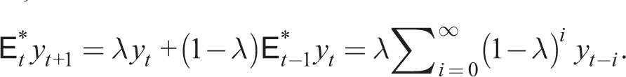
Thus, the expected value is a weighted average of past values of y_t. Gelain et al. (2019) find that such a rule in an estimated NK model fits the data better than RE. It should be noted that, as for k-level thinking, AE is not an SCEE.

Anufriev et al. (2015) propose a more general adaptive expectations rule:

$\begin{array}{l}{E}_t^{*}{y}_{t+1}=E_{t-1}^{*}{y}_t+{\lambda }_1\left(y_t-E_{t-1}^{*}{y}_t\right)\\ +{\lambda }_2\left(y_t-y_{t-1}\right);{\lambda }_2\in \left(-1,1\right).\end{array}$

(12)

This conforms with lab experiments, a speciality of Hommes and colleagues.

Concept IV: Euler Learning, Anticipated Utility and Individual Rational­ity: Throughout the learning literature, a division occurs between the Euler learning (EL) and anticipated utility (AU) approaches. EL is a more straightforward concept: in a linearized RE model featuring forward-looking expectations E_tx_{t + 1}, this expression is replaced with an adaptive expectations rule, usually a special case of (10) for example with λ = 0.

Turning to AU, a closely related literature develops the concept of internal rational­ity (IR) (see Adam & Marcet, 2011). Under both IR and AU, agents maximize utility under uncertainty, given their constraints and a consistent set of probability beliefs about payoff-relevant variables that are beyond their control or external. Then with IR, beliefs take the form of a well-defined probability measure over a stochastic process (the ‘fully Bayesian’ plan). See Eusepi and Preston (2011) for an RBC BR model with AU, Preston (2005) and Woodford (2013), who adopt a similar NK framework, and Branch and McGough (2018) provide a discussion of EL versus AU. Cogley and Sargent (2008) compare the IR with AU and encouragingly find that AU can be seen as a good approximation to IR.

Concept V: Inattention-Cognitive Discounting. Agents in the model perceive real­ity with some myopia and inattention as in Gabaix (2020). They are otherwise rational. An interesting discussant report is Cochrane (2016). This is related to finite-time horizon optimization as in Woodford (2018). Optimal policy applications are Levin and Sinha (2019) and Benchimol and Bounader (2019). An open economy application is Kolasa et al. (2022).

This subsection has reviewed a number of equilibrium concepts found in the literature that relax the RE assumption. In the rest of the paper, we will compare a standard NK that assumes RE with a number of behavioural counterparts. In the third and fourth sections, the behavioural model chosen is that with AU learning (concept IV). In the sixth section, the need for robust policy is demonstrated in its most clear fashion by comparing the RE model with EL (concept IV) and the inattention-myopia model (concept V). Finally, the section ‘Does Imperfect Information Improve Data Fit?’, reverts to AU in a comparison between RE with perfect and imperfect information.

RE and Bounded Rationality in the NK Model

Ultimately, our application will be conducted in terms of a linear NK RE model, under both perfect and imperfect information, and in a behavioural NK model. But first we step back to the underlying non-linear NK model and introduce the distinction between internal decisions and aggregate macro-variables. We start with the non-linear RE model and proceed from pure RE to pure BR in stages. The complete model set-up and its balanced growth steady state are summarized in Deák et al. (2023).

This subsection has reviewed a number of equilibrium concepts in the literature that go beyond RE.

Households

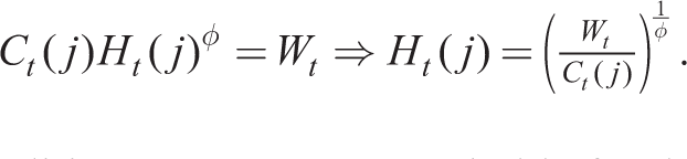
Household j chooses savings and between work and labour supply. Let C_t(j) be con­sumption and H_t(j) be the proportion of this available for work or leisure spent at the former. The single-period utility we choose, compatible with a balanced growth steady state, is

$U_t(j)=U\left(C_t(j),H_t\text{}(j)\right)=\text{log}\left(C_t(j)\right)-\frac{H_t\text{}{(j)}^{1+\varphi }}{1+\varphi }$

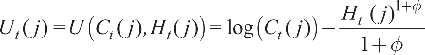
and the value function of the representative household at time t dependent on its assets B is

$V_t(j)=V_t\left(B_{t-1}(j)\right)=E_t{\displaystyle {\sum }_{s=0}^{\infty }{ϐ}^{s}U\left(C_{t+s}(j),H_{t+s}(j)\right).}$

The household’s problem at time t is to choose paths for consumption {C_t(j)}, labour supply {H_t(j)} and holdings of financial savings to maximize V_t(j) given by (13) given its budget constraint in period t

$\begin{array}{l}{B}_t(j)=R_t{B}_{t-1}(j)+W_t{H}_t(j)+{\Gamma }_t-C_t(j)\hfill \\ -T_t-\frac{\varpi }{2}{(B_{t-1}(j)-B)}^2.\hfill \end{array}$

(14)

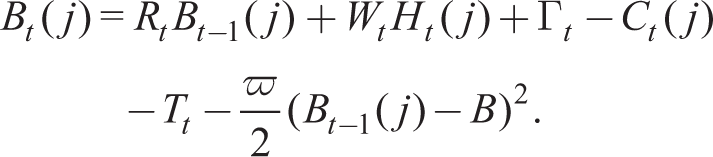
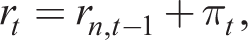
where B_t(j) is the given net stock of real financial assets at the end of period t, W_t is the wage rate, T_t are lump-sum taxes, Γ _t are profits from wholesale and retail firms owned by households. In order to allow for a wealth distribution heterogeneous agents introduced later and to achieve a stationary path for bond holdings, we introduce a portfolio adjust­ment cost. ¹ R_t is the real interest rate paid on assets held at the beginning of period t given by the Fischer equation

$R_t=\frac{R_{n,t-1}}{{\Pi }_t}.$

(15)

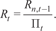
where R_n,t and Π _t are the nominal interest and inflation rates, respectively. W_t, R_n,t, Π _t and Γ _t are all exogenous to household j. As usual, all real variables are expressed relative to the price of final output. The standard first-order conditions are

$\begin{array}{l}{E}_t\left[{\Lambda }_{t,}{}_{t+1}\left(j\right)R_{t+1}\right]=1+\varpi \left(B_t(j)-B\right),\\ \frac{U_{H,t}(j)}{U_{C,t}(j)}=-W_t.\end{array}$

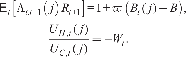
where Λ_{t,t + 1} (j) ≡ ϐ $\frac{U_{C,t+1}(j)}{U_{C,t}(j)}$ is the stochastic discount factor for household j, over the interval [t, t + 1]. For our choice of utility function $U_{C,t}=\frac{1}{{}_{Ct}}$ and U_H,t = $-H_t^{\varphi }$ so these become

$ϐE_t\frac{C_t(j)R_{t+1}}{C_{t+1}(j)}=1+\varpi \left(B_t(j)-B\right),$

(16)

$C_t(j)H_t{(j)}^{\varphi }=W_t\Rightarrow H_t(j)={\left(\frac{W_t}{C_t(j)}\right)}^{\frac{1}{\varphi }}.$

(17)

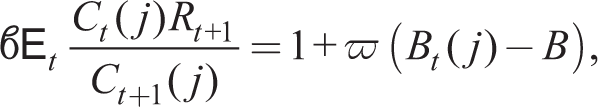
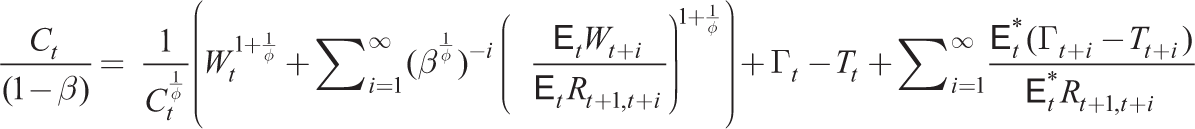
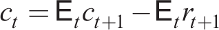
The first-order conditions up to now are suitable for the RE solution. We now express the solution in a form suitable for moving from a RE to a learning equilibrium. We consider the limit as ϖ → 0. Solving (14) forward in time and imposing the transversality condition on debt, we can write

$B_{t-1}(j)=\text{P}{\text{V}}_t\left(C_t(j)\right)-\text{P}{\text{V}}_t\left(W_t{H}_t(j)\right)-\text{P}{\text{V}}_t({\Gamma }_t)+\text{P}{\text{V}}_t(T_t).$

(18)

where the present (expected) value of a series $X\equiv {\left\{X_{t+1}\right\}}_{i=0}^{{}_{\infty }}$ at time t is defined by

$P{V}_t(X_t)\equiv E_t{\displaystyle {\sum }_{i=0}^{\infty }\frac{X_{t+i}}{R_{t,t+i}}}=\frac{X_t}{R_t}+\frac{1}{R_t}P{V}_t(X^{t+1}),$

(19)

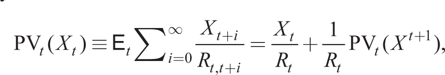
writing R_t,t+i = R_tR_{t + 1}R_{t + 2} • • • R_{t + i} as the real interest rate over the interval [t − 1, t + i].

The forward-looking budget constraint (18) holds for the representative household. If we allow RE and BR agents to borrow from or lend to one another, we must allow for B_t−1 = 0. Then in a symmetric equilibrium with C_t(j) = C_t and H_t(j) = H_t, (18) and (17) become

$\begin{array}{l}{B}_{t-1}=\text{P}{\text{V}}_t(C_t)-\text{P}{\text{V}}_t\frac{W_t{}^{1+\frac{1}{\varphi }}}{C_t^{\frac{1}{\varphi }}}-\text{P}{\text{V}}_t({\Gamma }_t)+\text{P}{\text{V}}_t(T_t),\\ H_t={\left(\frac{W_t}{C_t}\right)}^{\frac{1}{\varphi }}.\end{array}$

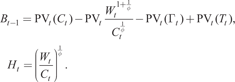
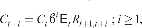
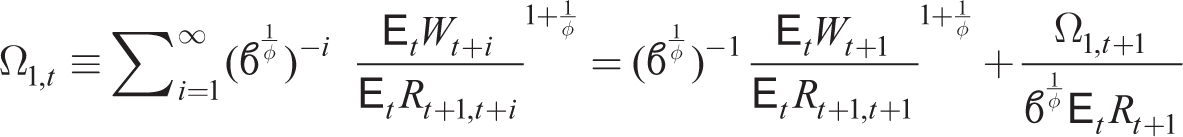
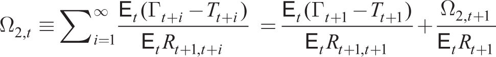
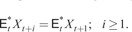
Solving (16) forward in time and using the law of iterated expectation, we have for i ≥ 1

$\frac{1}{C_t}={ϐ}^i{E}_t\frac{R_{t+1,t+i}}{C_{t+i}};i\ge 1.$

(20)

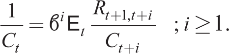
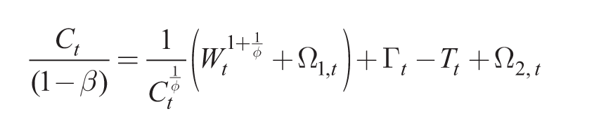
We now express the solution to the household optimization problem for C_t and H_t that are functions of point expectations ${\left\{E_t{W}_{t+i}\right\}}_{i=1}^{{}_{\infty }},$ ${\left\{E_t{R}_{t+1,t+i}\right\}}_{i=1}^{{}_{\infty }}$ and ${\left\{E_t{\Gamma }_{t+i}\right\}}_{i=0}^{{}_{\infty }}$ treated as exogenous processes given at time t. ² With point expectations, we use (20) to obtain the following optimal decision for C_{t + i} given point expectations E _t R_{t + 1,t+i}:

$C_{t+i}=C_t{ϐ}^i{E}_t{R}_{t+1,t+i};i\ge 1,$

(21)

$E_t(W_{t+i}{H}_{t+i})=\frac{(E_t{W}_{t+i})1+\frac{1}{\varphi }}{C_{t+i}^{\frac{1}{\varphi }}}.$

(22)

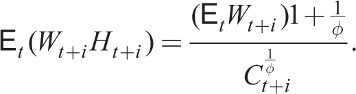
Substituting (21) and (22) into the forward-looking household budget constraint, using ${\displaystyle {\sum }_{i=0}^{\infty }{ϐ}^i}=\frac{1}{1-ϐ}$ and E _t R_t,t+i = R_tE _t R_{t + 1},_t+i for i ≥ 1, we arrive at

$\frac{C_t}{(1-\beta )}=\frac{1}{C_t^{\frac{1}{\varphi }}}\left(W_t^{1+\frac{1}{\varphi }}+{\displaystyle {\sum }_{i=1}^{\infty }{({\beta }^{\frac{1}{\varphi }})}^{-i}}{\left(\frac{E_t{W}_{t+i}}{E_t{R}_{t+1,t+i}}\right)}^{1+\frac{1}{\varphi }}\right)+{\Gamma }_t-T_t+{\displaystyle {\sum }_{i=1}^{\infty }\frac{E_t^{*}({\Gamma }_{t+i}-T_{t+i})}{E_t^{*}{R}_{t+1,t+i}}}$

which can be written in recursive form as

$\frac{C_t}{(1-\beta )}=\frac{1}{C_t^{\frac{1}{\varphi }}}\left(W_t^{1+\frac{1}{\varphi }}+{\Omega }_{1,t}\right)+{\Gamma }_t-T_t+{\Omega }_{2,t}$

${\Omega }_{1,t}\equiv {\displaystyle {\sum }_{i=1}^{\infty }({ϐ}^{\frac{1}{\varphi }})}{}^{-i}{\frac{E_t{W}_{t+i}}{E_t{R}_{t+1,t+i}}}^{1+\frac{1}{\varphi }}=({{ϐ}^{\frac{1}{\varphi }})}^{-1}{\frac{E_t{W}_{t+1}}{E_t{R}_{t+1,t+1}}}^{1+\frac{1}{\varphi }}+\frac{{\Omega }_{1,t+1}}{{ϐ}^{\frac{1}{\varphi }}{E}_t{R}_{t+1}}$

${\Omega }_{2,t}\equiv {\displaystyle {\sum }_{i=1}^{\infty }\frac{E_t({\Gamma }_{t+i}-T_{t+i})}{E_t{R}_{t+1,t+i}}}=\frac{E_t({\Gamma }_{t+1}-T_{t+1})}{E_t{R}_{t+1,t+1}}+\frac{{\Omega }_{2,t+1}}{E_t{R}_{t+1}}$

Consumption is then given by (23) assuming point expectations or by the symmetric form of the Euler equation (16) under full rationality (i.e., households know symmetric nature of equilibrium with C_t(j) = C_t). C_t is a function of rational point expectations ${\left\{E_t{W}_{t+i}\right\}}_{i=1}^{{}_{\infty }},$ ${\left\{E_t{R}_{t,t+i}\right\}}_{i=1}^{{}_{\infty }}$ and ${\left\{E_t{\Gamma }_{t+i}\right\}}_{i=1}^{{}_{\infty }}$ which can be treated as exogenous processes given at time t or as rational model-consistent expectations. Since E _t f (X_t) ≈ f (E _t (X_t)); E _t f (X_tY_t)) ≈ f (E _t (X_t)E _t (Y_t)) up to a first-order Taylor-series expansion, assuming point expectations is equivalent to using a linear approximation (given below), as is usually done in the literature.

Firms, Government Expenditures and Monetary Policy

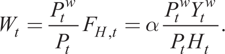
This section sets out the wholesalers and the retail sector which optimizes using Calvo-pricing contracts. We close the non-linear set-up with resource and balanced government budget constraints, a monetary policy rule and by specifying the structural shocks in the economy. Wholesale firms employ a Cobb–Douglas production function to produce a homogeneous output

$Y_t^w=F(A_t,H_t)=A_t{H}_t^{\alpha },$

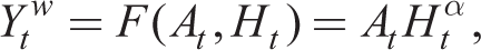
where A_t is total factor productivity. Profit-maximizing demand for labour results in the first-order condition

$W_t=\frac{P_t^w}{P_t}{F}_{H,t}=\alpha \frac{P_t^w{Y}_t^w}{P_t{H}_t}.$

(24)

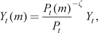
The retail sector costlessly converts a homogeneous wholesale good into a basket of differentiated goods for aggregate consumption

$C_t={\int }_0^1{C}_t{(m)}^{(\zeta -1)/\zeta }d{m}^{\zeta /(\zeta -1)},$

(25)

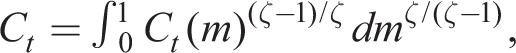
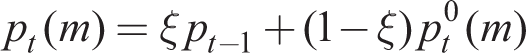
where ζ is the elasticity of substitution. For each m, the consumer chooses C_t(m) at a price P_t(m) to maximize (25) given total expenditure ${\int }_0^1{P}_t(m)C_t(m)dm$ . Assuming government services are similarly differentiated, this results in a set of demand equations for each differentiated good m with price P_t(m) of the form

$Y_t(m)={\frac{P_t(m)}{P_t}}^{-\zeta }{Y}_t,$

(26)

where $P_t={\left[{\displaystyle \int {}_0^1}{P}_t{(m)}^{1-\zeta }dm\right]}^{\frac{1}{1-\zeta }}.$ P_t is the aggregate price index. C_t and P_t are Dixit–Stigliz aggregates (see Dixit & Stiglitz, 1977).

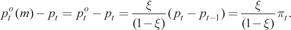
Following Calvo (1983), we assume that there is a probability of 1 − ξ at each period that the price of each retail good m is set optimally to P_t^O(m). If the price is not re-optimized, then it is held fixed. For each retail producer m, given its real marginal cost $M{C}_t=\frac{P_t^w}{P_t},$ the objective is at time t to choose {P_t^O(m)} to maximize discounted real profits

$E_t{\displaystyle {\sum }_{k=0}^{\infty }{\xi }^k}\frac{{\Lambda }_{t,t+k}}{P_{t+k}}{Y}_{t+k}(m)P_t^o(m)-P_{t+k}M{C}_{t+k}$

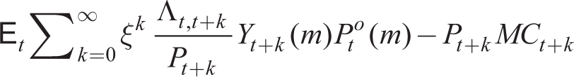
subject to (26), where ${\Lambda }_{t,}{}_{t+k}\equiv {ϐ}^k\frac{U_{C,t+k}}{U_{C,t}}$ , is the stochastic discount factor over the interval [t, t + k]. The solution to this is standard and given by

$\frac{P_t^o(m)}{P_t}=\frac{\zeta E_t{\displaystyle {\sum }_{k=0}^{\infty }{\xi }^k{\Lambda }_{t,t+k}{({\Pi }_{t,t+k})}^{\zeta }{Y}_{t+k}M{C}_{t+k}}}{{}^{(\zeta -1)}{E}_t{\displaystyle {\sum }_{k=0}^{\infty }{\xi }^k{\Lambda }_{t,t+k}{({\Pi }_{t,t+k})}^{\zeta }{({\Pi }_{t,t+k})}^{-1}{Y}_{t+k}}}$

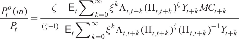
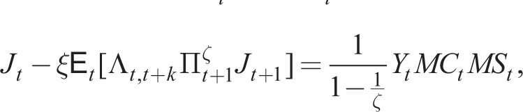
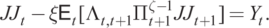
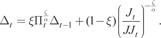
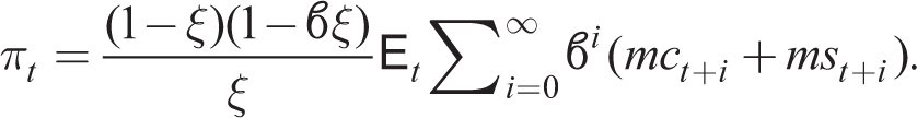
Denoting the numerator and denominator by J_t and JJ_t, respectively, and introducing a mark-up shock MS_t to MC_t, from Online Appendix D, we write in recursive form

$\frac{P_t^o(m)}{P_t}=\frac{J_t}{J{J}_t},$

(27)

$J_t-\xi E_t[{\Lambda }_{t,t+k}{\Pi }_{t+1}^{\zeta }{J}_{t+1}]=\frac{1}{1-\frac{1}{\zeta }}{Y}_{t}M{C}_{t}M{S}_t,$

(28)

$J{J}_t-\xi E_t[{\Lambda }_{t,t+1}{\Pi }_{t+1}^{\zeta -1}J{J}_{t+1}]=Y_t.$

(29)

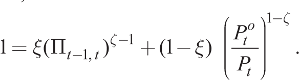
Using the fact that all resetting firms will choose the same price, by the law of large numbers, we can find the evolution of inflation given by

$1=\xi {({\Pi }_{t-1,t})}^{\zeta -1}+(1-\xi ){\left(\frac{P_t^o}{P_t}\right)}^{1-\zeta }.$

(30)

Price dispersion lowers aggregate output as follows. Market clearing in the labour market gives

$H_t={\displaystyle {\sum }_{m=1}^n{H}_t}(m)={{\displaystyle {\sum }_{m=1}^n\left(\frac{Y_t(m)}{A_t}\right)}}^{{}^{\frac{1}{\alpha }}}={\left(\frac{Y_t}{A_t}\right)}^{{}^{\frac{1}{\alpha }}}{{\displaystyle {\sum }_{m=1}^n\left(\frac{P_t(m)}{P_t}\right)}}^{\frac{-\zeta }{\alpha }}$

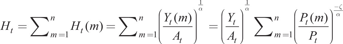
using (26). Hence equilibrium for good m gives $Y_t=\frac{Y_t^w}{{\Delta }_t^{\alpha }},$ where price dispersion is defined by

${\Delta }_t\equiv \left({{\displaystyle {\sum }_{m=1}^n\left(\frac{P_t(m)}{P_t}\right)}}^{-\frac{\zeta }{\alpha }}\right),$

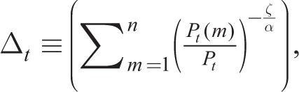
Assuming that the number of firms is large from Online Appendix E, we obtain the following dynamic relationship:

${\Delta }_t=\xi {\Pi }_t^{\frac{\zeta }{\alpha }}{\Delta }_{t-1}+(1-\xi ){\left(\frac{J_t}{J{J}_t}\right)}^{-\frac{\zeta }{\alpha }}.$

To close the model, we first require total profits from retail and wholesale firms, T _t , are remitted to households. This is given in real terms by

$T_t=\underset{\mathrm{retail}}{\underbrace{Y_t\frac{P_t^w}{P_t}{Y}_t^w}}+\underset{\mathrm{Wholesale}}{\underbrace{\frac{P_t^w}{P_t}{Y}_t^w-W_t{H}_t}}=Y_t-\alpha \frac{P_t^w}{P_t}{Y}_t^w$

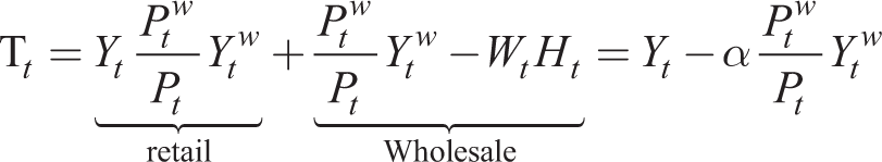
using the first-order condition (24). Then to complete closure, we have resource and balanced government budget constraints

$Y_t=C_t+G_t=C_t+T_t$

where G_t is an exogenous demand process, and a monetary policy rule for the nominal interest rate given by the following implementable Taylor-type rule

$\log \left(\frac{R_{n,t}}{R_n}\right)=\rho {}_{\text{}\text{}r\text{}\text{}\text{}\text{}}\text{l}\text{og}\left(\frac{R_{n,t-1}}{R_n}\right)+(1-{\rho }_r)(\theta {}_{\text{}\text{}\pi \text{}\text{}\text{}\text{}}\text{l}\text{og}\left(\frac{{\Pi }_t}{{\Pi }_{targ,t}}\right)+{\theta }_y\log \left(\frac{Y_t}{Y}\right)+{\theta }_{dy}\log \left(\frac{Y_t}{Y_{t-1}}\right))+{\in }_{MP,t}$

(31)

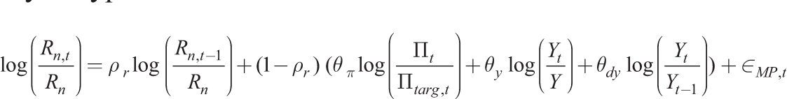
and ε_MP,t is an i.i.d. shock to monetary policy. Π _targ,t is a time-varying inflation target and together with A_t, G_t and MS_t follows an AR(1) process. This completes the model.

Recovering the NK Workhorse Model

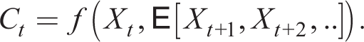
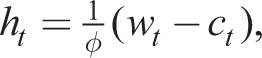
We now show that the linearized form of the non-linear model about the steady state reduces to the standard workhorse model where rational expectations E _t y_{t + 1} and E _t π_{t + 1} or non-RE E* _t y_{t + 1} and E* _t π_{t + 1} can be treated as expectations by individual households and firms, respectively, of aggregate future output and inflation. We consider the linearized form of the above set-up about a zero inflation and growth deterministic steady state. We also ignore lending or borrowing between RE and BR agents. With RE, the household j’s first-order conditions take one of two forms. First, linearizing (23) we have

$\begin{array}{l}{\alpha }_1{c}_t(j)={\alpha }_2{w}_t+{\alpha }_3({\omega }_{2,t}+r_t)+{\alpha }_4{\omega }_{1,t},\hfill \\ {\omega }_{1,t}={\alpha }_5{E}_t{w}_{t+1}-{\alpha }_6{E}_t{r}_{t+1}+ϐE_t{\omega }_{1,t+1},\hfill \\ {\omega }_{2,t}=(1-ϐ)({\gamma }_t-g_t)-r_t+ϐE_t{\omega }_{2,t+1},\hfill \\ {\gamma }_t=\frac{1}{{\gamma }_y}{y}_t-\frac{\alpha }{{\gamma }_y}(w_t+h_t),\hfill \end{array}$

(32)

from (23) where lower case variables x_t = log(X_t/X), where X is the steady state of $X_t;c_y\equiv \frac{C}{y},{\gamma }_y\equiv \frac{\Gamma }{y},g_y\equiv \frac{G}{y}and{\gamma }_t$ is exogenous profit per household (a function of aggregate consumption and hours). Positive coefficients are given by ${\alpha }_1\equiv 1+\frac{\alpha }{\varphi },c_y{\alpha }_2\equiv (1-ϐ)(1+\frac{1}{\varphi })\frac{\alpha }{c_y},{\alpha }_3\equiv \frac{{\gamma }_y}{c_y},{\alpha }_4\equiv \frac{ϐ\alpha }{c_y},{\alpha }_5\equiv (1-ϐ)(1+\frac{1}{\varphi })\text{and}{\alpha }_6\equiv (1+\frac{1}{\varphi }).$ ${\alpha }_1\equiv 1+\frac{\alpha }{\varphi },c_y{\alpha }_2\equiv (1-ϐ)(1+\frac{1}{\varphi })\frac{\alpha }{c_y},{\alpha }_3\equiv \frac{{\gamma }_y}{c_y},{\alpha }_4\equiv \frac{ϐ\alpha }{c_y},{\alpha }_5\equiv (1-ϐ)(1+\frac{1}{\varphi })\text{and}{\alpha }_6\equiv (1+\frac{1}{\varphi }).$ Alternatively, from the Euler equation (16):

$c_t=E_t{c}_{t+1}-E_t{r}_{t+1}$

(33)

in a symmetric equilibrium. Under RE, (32) or (33) leads to the same equilibrium, but under BR, this is no longer the case.

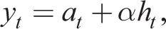
Linearizing the household supply of hours decision, the resource constraint and the Fisher equation, we have

$y_t=(1-g_y)c_t+g_y{g}_t,$

(34)

$r_t=r_{n,t-1}+{\pi }_t,$

(35)

$h_t=\frac{1}{\varphi }(w_t-c_t),$

(36)

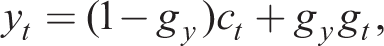
which completes the decisions of the household. Substituting out for c_t from (34)

$y_t=E_t{y}_{t+1}-(1-g_y)E_t{r}_{t+1}+g_y(E_t{g}_{t+1}-g_t).$

(37)

Turning to the supply side, for the wholesale sector

$y_t=a_t+\alpha h_t,$

(38)

$m{c}_t=w_t-y_t+h_t.$

(39)

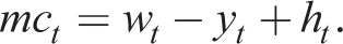
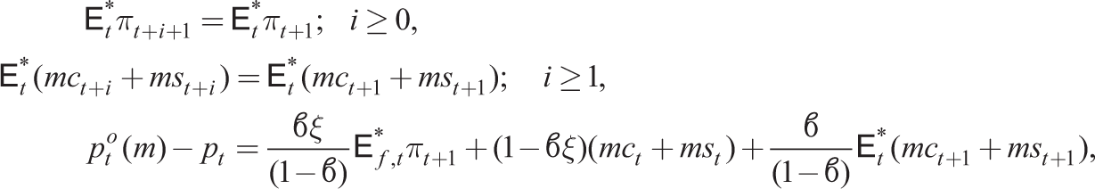
For retail firm m, linearizing the pricing dynamics (27)–(29) about a zero net equation steady state and solving forwards, we have

$\begin{array}{l}{p}_t^o(m)-p_t=ϐ\xi E_t[{\pi }_{t+1}+p_{t+1}^o(m)-p_{t+1}]+(1-ϐ\xi )(m{c}_t+m{s}_t)\hfill \\ =E_t{\displaystyle \sum }_{i=0}^{\infty }{(ϐ\xi )}^i[ϐ\xi {\pi }_{t+i+1}+(1-ϐ\xi )(m{c}_{t+i}+m{s}_{t+i})].\hfill \end{array}$

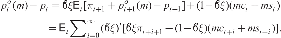
Then, in a symmetric equilibrium, we have

${\pi }_t=\frac{(1-\xi )}{\xi }{E}_t{\displaystyle \sum }_{1=0}^{\infty }{(ϐ\xi )}^i[ϐ\xi {\pi }_{t+i+1}+(1-ϐ\xi )(m{c}_{t+i}+m{s}_{t+i}),$

where E _t [π_t+i+1] and E _t [mc_{t + i} + ms_{t + i}] are expectations of aggregate inflation and real marginal costs, both variables exogenous to individual price-setters. However, if price-setters know they are identical they know the aggregate price level over non-optimizing and optimizing firms

$p_t(m)=\xi p_{t-1}+(1-\xi )p_t^0(m)$

(42)

to obtain in a symmetric equilibrium

$p_t^o(m)-p_t=p_t^o-p_t=\frac{\xi }{(1-\xi )}(p_t-p_{t-1})=\frac{\xi }{(1-\xi )}{\pi }_t.$

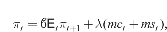
Then, substituting back into (40), we arrive at

${\pi }_t=\frac{(1-\xi )(1-ϐ\xi )}{\xi }{E}_t{\displaystyle {\sum }_{i=0}^{\infty }{ϐ}^i(m{c}_{t+i}+m{s}_{t+i})}.$

which omits learning about aggregate inflation. Under RE, (41) and (43) are equivalent. (43) is equivalent to

${\pi }_t=ϐE_t{\pi }_{t+1}+\lambda (m{c}_t+m{s}_t),$

(44)

where $\lambda =\frac{(1-\xi )(1-\ell \xi )}{\xi }$ , which is the familiar linearized Phillips curve expressed in terms of the real marginal cost mc_t and the mark-up shock ms_t. Substituting for the former from (38) and (39), we arrive at

${\pi }_t=ϐE_t{\pi }_{t+1}+\lambda \frac{1+\varphi }{\alpha }(y_t-a_t)-\frac{g_y}{1-g_y}{g}_t+m{s}_t,$

(45)

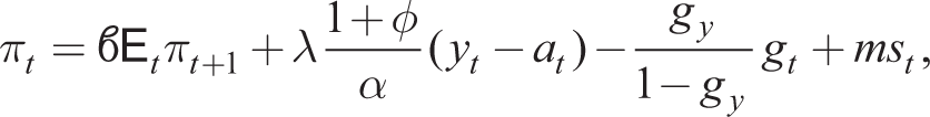
where we note that y_t − a_t is the output gap. Equations (37), (45) and the Taylor rule (31) constitute the 3-equation NK RE model in output, inflation and the nominal interest rate given exogenous shock processes for g_t, ms_t and the monetary shock. A simpler form omits government spending g_t so g_y = 0 and replaces the aggregate demand shock in (45) with an exogenous process that can be thought of as a risk premium shock to the Fischer equation (35).

The form of the Phillips curve (43) is often used in the behavioural NK literature (see, e.g., De Grauwe, 2012b), but as we have shown, this assumes that firms know they are identical. In our BR model with AU learning, we use (32) and (41), which do not make this assumption.

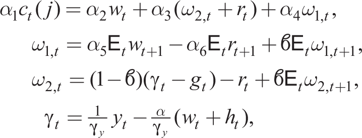
AU Learning and Market-consistent Information

With AU learning, our learning model is one where agents make fully optimal decisions given their individual specification of beliefs but have no macroeco­nomic model to form expectations of aggregate variables. We draw a clear distinction between aggregate and internal quantities so that identical agents in our model are not aware of this equilibrium property (nor any others).

To close the model, we need to specify the manner in which households and firms form their expectations. To do so, we assume that variables which are local to the agents, in a geographical sense, are observable within the period, whereas variables that are strictly macroeconomic are only observable with a lag. This categorization regarding information about the current state of the economy follows Nimark (2014). He distinguishes between the local information that agents acquire directly through their interactions in markets and statistics that are collected and summarized, usually by governments, and made available to the wider public. 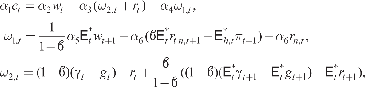³ The policy rate is announced by the central bank, so it is observed without a lag and it is common knowledge. Given this, we assume an adaptive expectations forecasting rule given below by (47) and (48) about variables external to agents’ decisions. Let x_t = r_t, r_n,t, π_t, w_t, γ_t, g_t, then household expectations are given by

$E_t^{*}{X}_{t+i}=E_t^{*}{X}_{t+1};i\ge 1.$

(46)

Expressing E _t ω_{1,t + 1} and E _t ω_{2,t + 1} in (32) as forward-looking summations and using (46), we arrive at the individual learning consumption equation

$\begin{array}{l}{\alpha }_1{c}_t={\alpha }_2{w}_t+{\alpha }_3({\omega }_{2,t}+r_t)+{\alpha }_4{\omega }_{1,t},\\ {\omega }_{1,t}=\frac{1}{1-ϐ}{\alpha }_5{E}_t^{*}{w}_{t+1}-{\alpha }_6(ϐE_t^{*}{r}_{tn,t+1}-E_{h,t}^{*}{\pi }_{t+1})-{\alpha }_6{r}_{n,t},\\ {\omega }_{2,t}=(1-ϐ)({\gamma }_t-g_t)-r_t+\frac{ϐ}{1-ϐ}((1-ϐ)(E_t^{*}{\gamma }_{t+1}-E_t^{*}{g}_{t+1})-E_t^{*}{r}_{t+1}),\end{array}$

which is now expressed in terms of one-step-ahead forecasts by the standard adaptive expectations rule ⁴ :

$E_t^{*}{x}_{t+1}=E_{t-1}^{*}{x}_t+{\lambda }_x(x_{t-j}-E_{t-1}^{*}{x}_t);x=w,r_n,\pi ,\gamma -g;j=0,1$

(47)

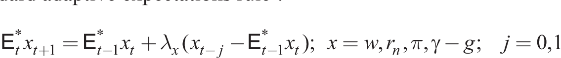
Households make inter-temporal decisions for their consumption and hours supplied given adaptive expectations of the wage rate, the nominal interest rate, inflation and profits. These macro-variables may in principle be observed with or without a one-period lag (j = 1, 0), but as stated earlier, we assume j = 0 for market-specific variables w_t, γ_t − g_t, and j = 1 for aggregate inflation π_t. However, we assume the current nominal interest rate, r_n,t, is announced and therefore also observed without a lag.

We distinguish household and firm expectations $E_{h,t}^{{}_{*}}{\pi }_{t+1,}{E}_{f,t}^{{}_{*}}{\pi }_{t+1}.$ Then for retail firm m.

$\begin{array}{l}{E}_t^{*}{\pi }_{t+i+1}=E_t^{*}{\pi }_{t+1};i\ge 0,\\ E_t^{*}(m{c}_{t+i}+m{s}_{t+i})=E_t^{*}(m{c}_{t+1}+m{s}_{t+1});i\ge 1,\\ p_t^o(m)-p_t=\frac{ϐ\xi }{(1-ϐ)}{E}_{f,t}^{*}{\pi }_{t+1}+(1-ϐ\xi )(m{c}_t+m{s}_t)+\frac{ϐ}{(1-ϐ)}{E}_t^{*}(m{c}_{t+1}+m{s}_{t+1}),\end{array}$

where again one-step-ahead forecasts are given by the adaptive expectations rule:

$E_t^{*}{x}_{t+i}=E_{t-1}^{*}{x}_t+{\lambda }_x(x_{t-j}-E_{t-1}^{*}{x}_t);x=\pi ,(mc+ms);j=0,1.$

(48)

Retail firms make inter-temporal decisions for their price and output given adaptive expectations of the aggregate inflation rate and their post-shock real marginal shock wage rate. As before, these variables may be observed with or without a one-period lag (j = 1, 0), but for aggregate inflation, we assume j = 1 as for households, but j = 0 for the market-specific variable mct. Note that we can in principle distinguish between households’ and firms’ expectations of inflation.

Heterogeneous Expectations and Reinforcement Learning

There is a growing literature within behavioural macro-models based on the Brock and Hommes (1997) framework where agents learn from each other through reinforcement learning. More recently, DeGrauwe has used this framework based on the 3-equation linearized workhorse NK model.

RE expectations are then replaced with boundedly rational (BR) with simple fore casting rules; that is, replace E _t (RE) with E^* _t (non-RE). This is the Euler equation learning (EL) approach. There are two types of agents with different forecasting rules. Both can use simple misspecified forecasting rules as in De Grauwe (2012b). One set can be rational as in Branch and McGough (2010) and Massaro (2013). See also Young (2004), Choi et al. (2009), De Grauwe (2011, 2012a) and Hommes et al. (2019). Jump and Levine (2019) provide a survey. All these papers feature misspecified equilibria which are not SCEE: the PLM is inconsistent with the ALM. There is a major modelling issue: Euler learning versus anticipated utility.

Heterogeneous Expectations with Fixed Proportions of RE and BR Agents

Now we turn to the heterogeneous expectations model with BR(AU) agents alongside RE agents with fixed proportions of each type. We assume all RE agents know the composite model. In addition, we impose informational inconsistency by assuming they have the same II set as the BR(AU) agents. The latter do not know the model, but do make individually optimal decisions given individual observations of the states and belief formations. The composite RE–BR model then has an equilibrium (in non-linear form)

$\begin{array}{l}{H}_t^d=n_{h,t}{(H_t^s)}^{RE}+(1-n_{h,t}){(H_t^s)}^{BR},\hfill \\ C_t=n_{h,t}{(C_t)}^{RE}+(1-n_{h,t}){(C_t)}^{BR}=Y_t-G_t,\hfill \\ \frac{p_t^o}{p_t}=n_{f,t}{\frac{p_t^o}{p_t}}^{RE}+(1-n_{f,t}){\frac{p_t^o}{p_t}}^{BR},\hfill \end{array}$

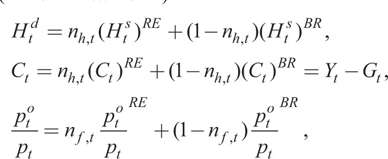
Zero net wealth in aggregate implies that $n_{h,t}{B}_t^{{}_{RE}}=-(1-n_{h,t})B_t^{{}_{RE}}.$ We consider the properties of the model with fixed exogenous proportions of RE and BR agents.

Figure 1.

RE vs RE–BR Composite Expectations with n_h = n_f = 0.5, λ_x = 0.25, 1.0; Taylor rule with ρ_r = 0.7, υ_pi = 1.5 and υ_y = 0.3, υ_dy = 0; Monetary Policy Shock.

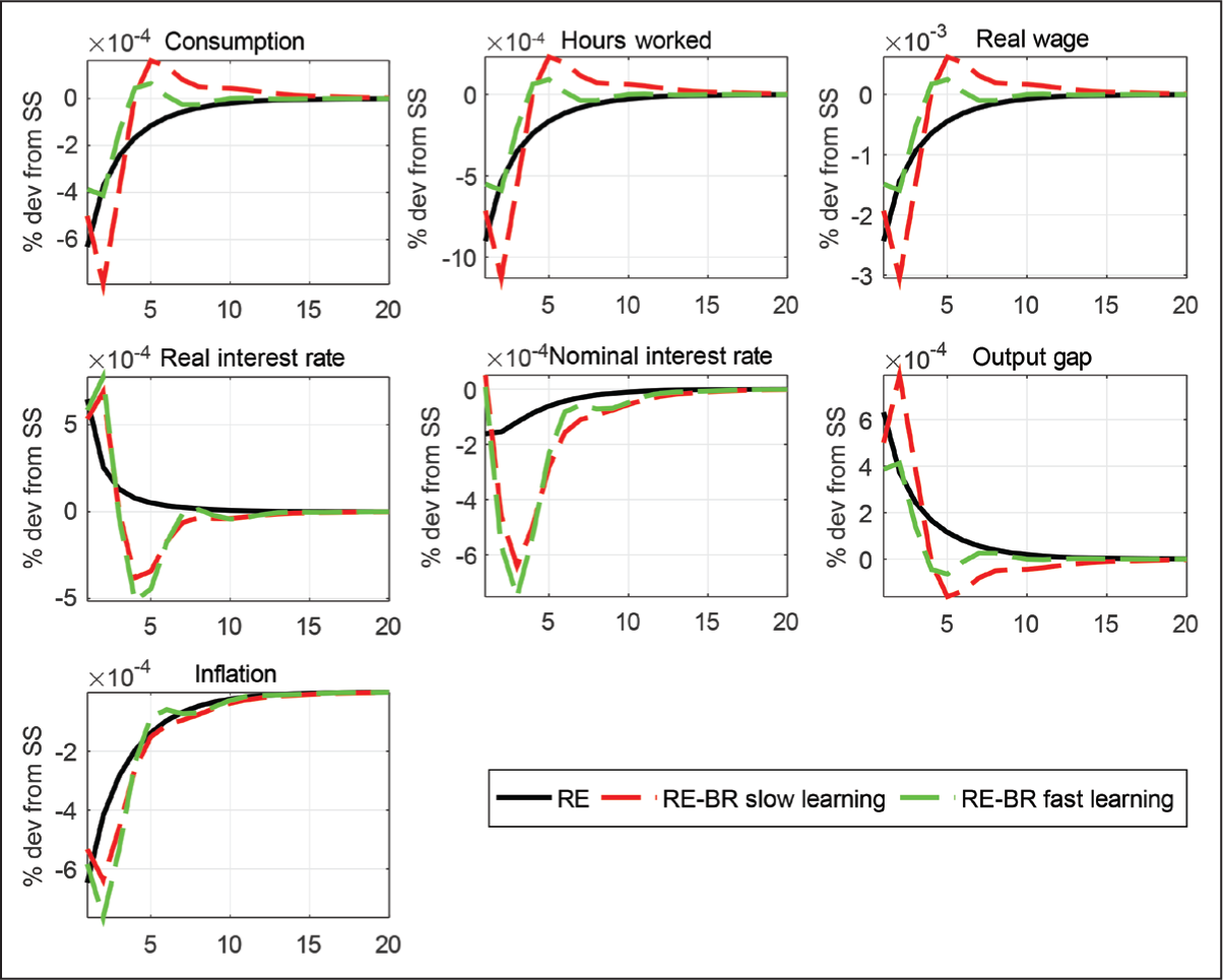
For our model of BR with AU, Figure 1 plots the impulse response functions (IRFs) with standard parameters for the rule for a shock to monetary policy under fast and slow learning. Not surprisingly, fast learning sees an IRF converge faster to the RE case, but in either case BR introduces more persistence compared with RE. This suggests that this feature should lead to a better fit of the data without relying on other persistence mechanisms (shocks, habit or price indexing). This we examine in the estimation of our model. ⁵

Endogenous Proportions of Rational and Non-rational Agents: Reinforcement Learning

Up to now we assume that the proportions of rational and non-rational agents n_y,t and n_π,t are exogenous. As in Massaro (2013), in the estimation and main conclusions that follow, we retain this assumption, but in this sub section, we explore the extension that endogenizes these decisions by agents. Following Brock and Hommes (1997) and the reinforcement learning literature in general, these can be chosen as follows:

$n_{x,t}=\frac{\exp (-\gamma {\Phi }_{x,t}^{RE}(\left\{x_t\right\}))}{\exp (-\gamma {\Phi }_{x,t}^{RE}(\left\{x_t\right\}))+\exp (-\gamma {\Phi }_{x,t}^{AE}(\left\{x_t\right\}))},$

(49)

where $-{\Phi }_{x,t}^{RE}(\{x_t\})\text{and}-{\Phi }_{x,t}^{AE}(\{x_t\})$ are ‘fitness’ measures, respectively, of the forecast performance of the rational and non-rational predictor of outcome {x_t} = {y_t}, {π_t} given by a discounted least-squares error predictor

${\Phi }_{x,t}^{RE}(\{x_t\})={\mu }_{RE}{\Phi }_{x,t-1}^{RE}(\{x_t\})+(1-{\mu }_{RE})({[x_t-E_{t-1}{x}_t]}^2+C_x),$

(50)

${\Phi }_{x,t}^{AE}(\{x_t\})={\mu }_{AE}{\Phi }_{x,t-1}^{AE}(\{x_t\})+(1-{\mu }_{AE})({[x_{t-j}-E_{t-1-j}^{\ast }{x}_{t-1}]}^2;j=0,1,$

(51)

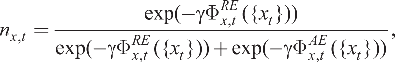
where ρ_RE and ρ _AE capture the memory of the agents forming RE and AE (a measure of forgetfulness of past observations). C_x represents the relative costs of being rational in learning about variable x_t. Thus, the proportion of rational agents in the steady state is given by

$n_x=\frac{\exp (-\gamma C_x)}{\exp (-\gamma C_x)+1},$

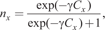
which is pinned down by the γC_x.

A complete treatment of the model would require a departure from the linear Kalman filter solution for the II case for which we exploit the closed-form saddlepath solution that Pearlman et al. (1986) show both exists and is unique. We have also exploited the convenience of linear Bayesian estimation. In what follows we confine ourselves to the RE PI case and use the linear estimates obtained up to now.

Agents with reinforcement learning that now have proportions of rational households (n_h,t) and firms (n_f,t) are given by (49). Table 1 provides a third-order perturbation solution of the non-linear NK RE(PI)-BR model. We use the Bayesian estimation of the linear model in ‘the first, second, third section’ etc. where the model is linearized and the proportions n_h,t and n_f,t are fixed. Non-linear estimation would be required to pin down the parameters n_h, n_f in the steady state, and ${\mu }_h^{RE,BR},{\mu }_f^{RE,BR}$ and γ in the reinforcement learning process and goes beyond the scope of this article. So here we impose them as reported in the table. We also scale the estimated standard deviations of the shocks using a parameter σ = 1, 2.

Table 1.

Third-order Solution of the Estimated NK RE(PI)-BR Model; ${\mu }_h^{{}_{RE}}={\mu }_h^{{}_{BR}}={\mu }_f^{{}_{RE}}={\mu }_f^{{}_{BR}}=0;$ ; γ = 1, 100, 1,000.

Variable	Stochastic Mean	Standard Deviation (%)	Skewness	Kurtosis
$\frac{C_t}{C}$	0.9993	2.47	0.2792	0.0371
$\frac{H_t}{H}$	1.0002	0.19	0.0192	0.0327
$\frac{w_t}{w}$	0.9996	2.15	0.2771	0.0215
$\frac{{\Pi }_t}{\Pi }$	0.9999	0.46	0.0159	0.0645
$\frac{R_{n,t}}{R_n}$	0.9999	0.46	0.0070	0.0651
${\Phi }_{h,t}^{RE}-C_h$	–0.000065	0.000020	–0.7589	0.9487
${\Phi }_{h,t}^{AE}$	–0.000084	0.000054	–1.8238	5.7852
${\Phi }_{f,t}^{RE}-C_f$	–0.000011	0.000009	–0.7203	0.7834
${\Phi }_{f,t}^{AE}$	–0.000069	0.000053	–2.2156	8.8686
nh,t(γ = 1; σ = 1)	0.093301	0.000004	1.8039	6.0897
nf,t(γ = 1; σ = 1)	0.098603	0.000004	2.2688	9.2725
nh,t(γ = 100; σ = 1)	0.094221	0.003634	1.8039	6.0897
nf,t(γ = 100; σ = 1)	0.101751	0.004303	2.2688	9.2725
nh,t(γ = 1000; σ = 1)	0.102506	0.036343	1.8039	6.0897
nf,t(γ = 1000; σ = 1)	0.130105	0.043030	2.2688	9.2725
nh,t(γ = 1000; σ = 2)	0.129993	0.146939	1.8403	6.6096
nf,t(γ = 1000; σ = 2)	0.224367	0.174046	2.3668	10.5098

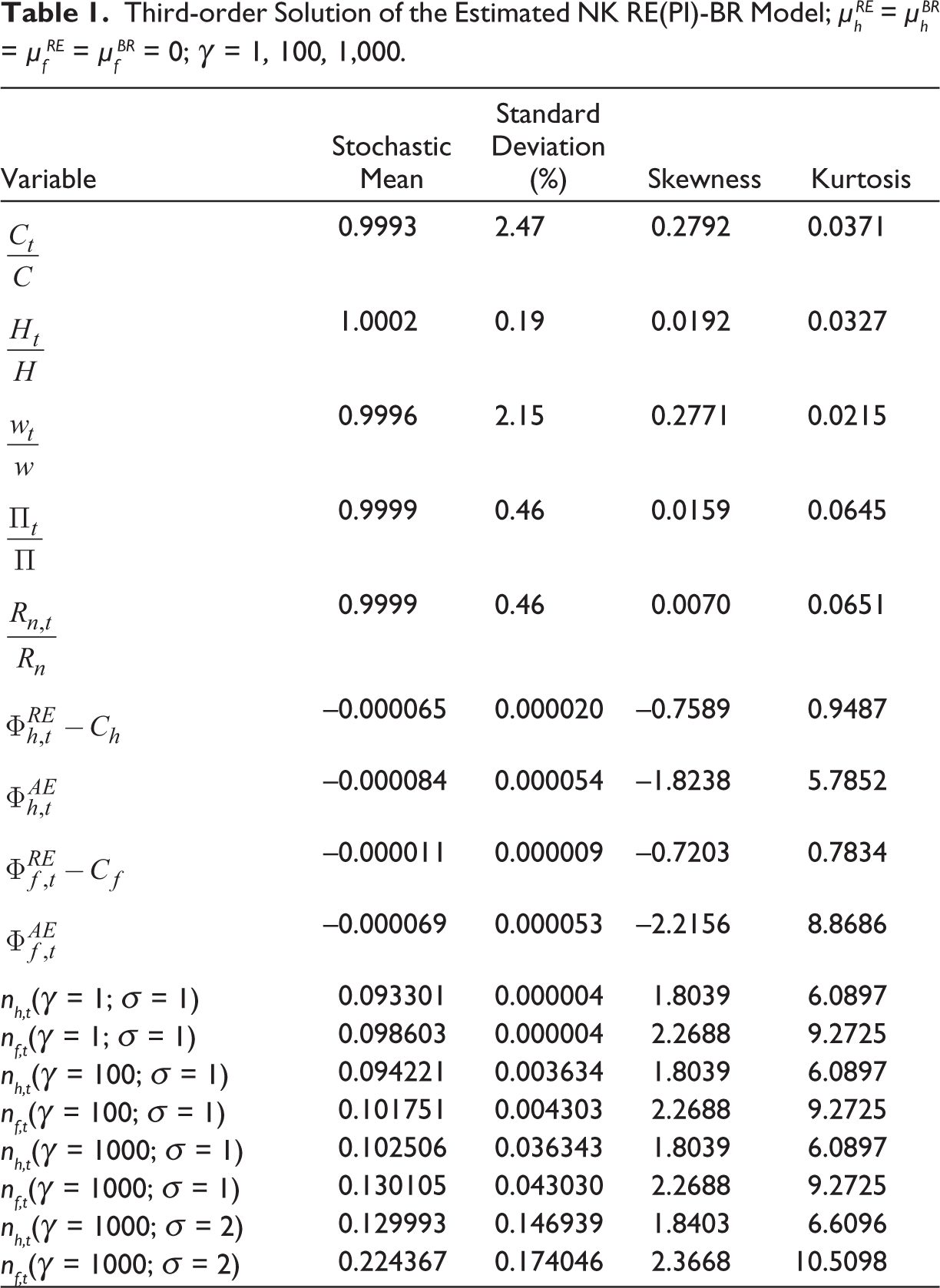
The main results from these simulations are as follows. First, reinforcement learning introduces high kurtosis and skewness ⁶ in macro variables. Second, reinforcement learning coupled with higher volatility of exogenous shocks results in the numbers of rational agents increasing from the estimated deterministic steady-state value of 0.093 and 0.099 to 0.13 and 0.22 for households and firms, respectively, in the stochastic steady state. Third, given that bounded rationality is a welfare-reducing friction in these models, it follows that volatility can actually be welfare-increasing in our homogeneous expectations setting.

Perfect Versus Imperfect Information

The seminal paper on the general solution of linear RE models assuming perfect (aka full) information (the standard assumption) is provided by Blanchard and Kahn (1980) showing existence and conditions for uniqueness.

Perfect information means that at time t, all agents have full information about all the state variables of the system. Conventional estimation is performed under the assumption that agents have perfect information (including shocks), but econometricians do not. Thus there is an inconsistency about information available to agents and econometricians. Here we adopt the informational consistency principle, which states that agents and econometricians have the same imperfect information set. Thus if econometricians do not have current data on technical progress, then it is assumed that agents also do not have this.

Angeletos and Lian (2016) provide an important survey paper on what they refer to as incomplete information literature. Here a comment on terminology is called for. Our use of perfect/imperfect information corresponds to the standard use in dynamic game theory when describing the information of the history of play driven by draws by nature from the distributions of exogenous shocks. Complete/incomplete information refers to agent’s beliefs regarding each other’s payoffs and information sets. In our set-up, the latter informational friction is absent.

Minford and Peel (1983) were the first to show the importance of information sets for the IRFs and second moments of RE models. Pearlman et al. (1986) generalized this for the general linear model. Pearlman (1992) extended this to optimal policy for fully optimal and time-consistent rules. Kalman filter ‘learning’ is central; see Hamilton (1994) and Adam and Billi (2006). Pearlman and Sargent (2005) and Levine et al. (2023) extend the representative agent II solution to a heterogeneous agent framework with diffuse information and show that a finite-space solution is available. The solution procedure of Pearlman et al. (1986) is applied in Collard and Dellas (2004, 2006, 2007), Levine et al. (2012a, 2012b) and Cantore et al. (2015). Following on from Pearlman (1992), Svensson and Woodford (2001, 2003) investigate the properties of the optimal solution under II. Ellison and Pearlman (2011) show e-stability (convergence to RE equilibrium under imperfect information). II is distinguished from the rational inattention literature, in which information assumptions are imposed, whereas in the latter, the acquisition of information was endogenous. See Sims (2005) and Mackowiak and Wiederholt (2009, 2011).

Why II? Some Empirical Motivation

• Evidence from Forecast Surveys, Outcomes and Forecast Errors. See Coibion and Gorodnichenko (2012, 2015), Coibion et al. (2018) and Angeletos and Sastry (2020). The main finding: Initial under-reaction of beliefs in response to shocks followed by delayed overreaction.

• Bayesian Estimation of DSGE Models. II improves data fit compared with PI. See Collard et al. (2009) and Levine et al. (2012a).

Real Effects of Monetary Policy

II with the diverse information pricing model predicts highly persistent effects on real activity in contrast to the Phelps–Lucas model. This results in a hierarchy of expectations as seen in beauty contest models (forecasting the forecasts of others). To show this, we consider the following model from Woodford (2003).

In log-linear form, let q_t be an exogenous process for nominal income and y_t be output. Then the Lucas Philips curve is

$\begin{array}{l}{\gamma }_t=\xi (q_t-E_t{q}_t)\text{with}\text{common}\text{knowlege}\\ \text{=}{\displaystyle {\sum }_{k=1}^{\infty }\xi {(1-\xi )}^{k-1}(q_t-q_t^{(k)})\text{with}\text{diverse}\text{information}}\end{array}$

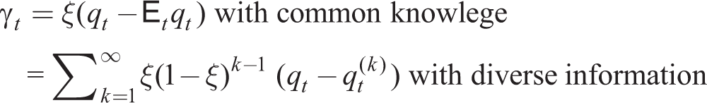
where q_t^(k) ≡ Ē _t [q_t^k–1] is the k-order average expectation of the k–1 order average expectation. These higher-order expectations result in persistent effects of surprises without introducing other features such as Calvo or Rotemberg pricing.

Empirical Results

The Wilderness of Non-rationality

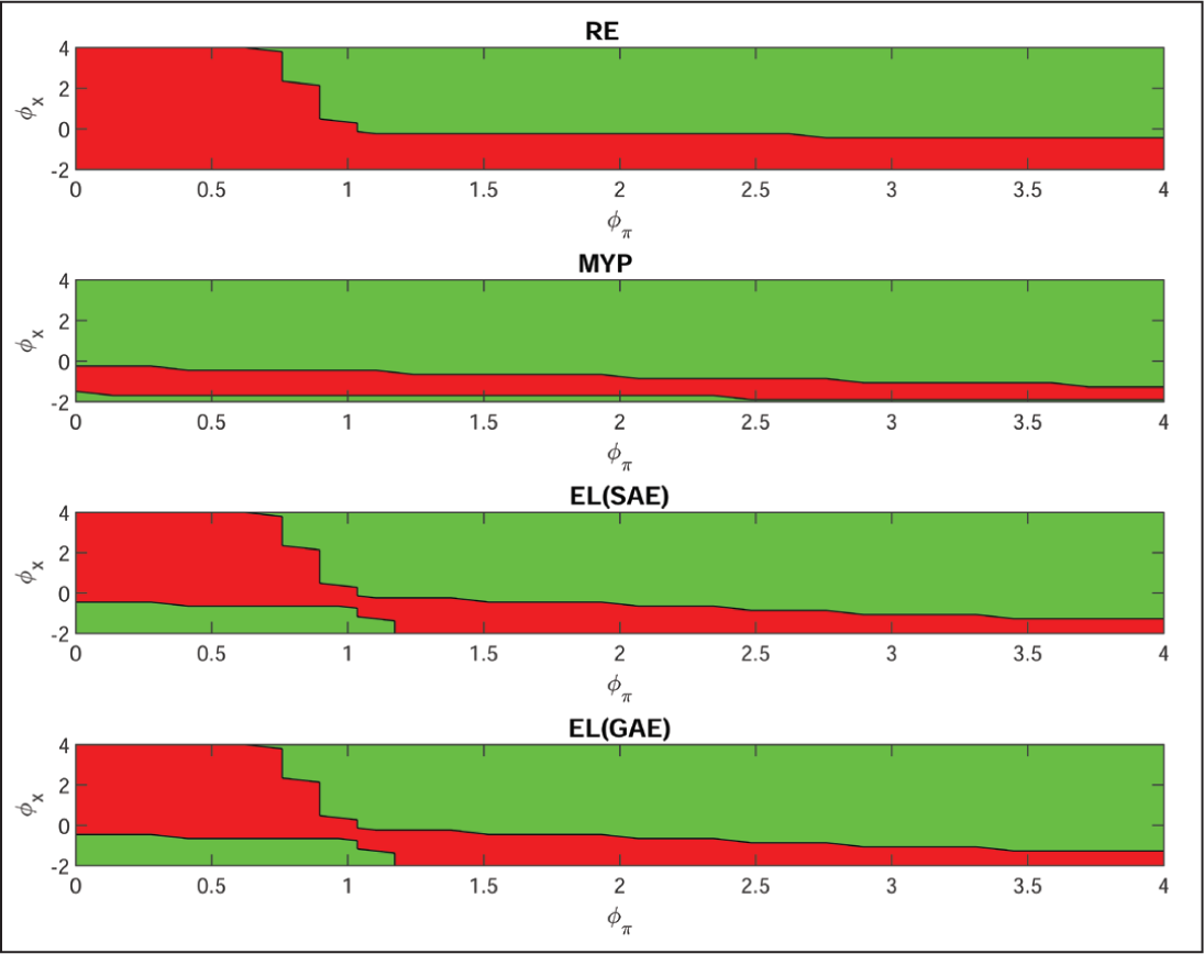
This section demonstrates the need for robust policy design using a special case of the four models for which in a balanced growth deterministic steady state both net inflation and growth is zero. Then about such a steady state, the linearized models take the form:

Myopia-RE models

$x_t=M{E}_t[x_{t+1}]-(r_{n,t}-E_t{\pi }_{t+1}-r_{n,t}^{\ast })+u_t,(\text{IS}\text{curve})$

(52)

${\pi }_t=ϐM^f{E}_t[{\pi }_{t+1}]+k{x}_t,(\text{Phillips}\text{curve})$

(53)

$r_{n,t}=r_{n,t}^{\ast }+{\vartheta }_{\pi }{\pi }_t+{\vartheta }_x{x}_t(\text{Taylor}\text{interest}\text{rate}\text{rule})$

(54)

where x_t is the output gap, π_t is the gross inflation rate, r_n,t is the nominal interest given by the original Taylor rule (ϑ_π = 1.5, ϑ_x = 0.2), r^*_n,t is its natural rate, u_t is a demand push shock, m = M^f = 1 for the RE case and M < 1, M^f < 1 for the myopia case.

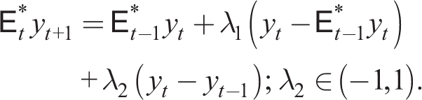
To formulate possible heuristic rules that encompass those in these papers, we draw upon the general form of adaptive expectations from Anufriev et al. (2015) discussed in the ‘Behavioural Macro models’ section that takes the log-linear general form

$E_t^{\ast }(y_{t+1})={[E_{t-1}^{\ast }(y_t)]}^{1-{\lambda }_y^1}{[y_t]}^{{\lambda }_y^1+{\lambda }_y^2}{[y_{t-1}]}^{-{\lambda }_y^2},0<{\lambda }_y^1<1,-1<{\lambda }_y^2<1.$

(55)

This encompasses simple adaptive expectations ( ${\lambda }_y^2=0$ ), ‘trend extrapolation’ ( ${\lambda }_y^1=0$ ), and a ‘fundamentalist’ rule $({\lambda }_y^2={\lambda }_y^1=0)\text{for}\text{which}{E}_t^{\ast }(y_{t+1})=E_{t-1}^{\ast }(y_t)=$ the model’s steady state. In the latter paper parameters ${\lambda }_y^1\mathrm{and}{\lambda }_y^2$ are modelled as changing overw time, as the agents repeatedly fine-tune the rule to adapt to the specific market conditions. In their paper, this learning is embodied as a heuristic optimization with a genetic algorithm procedure and introduces the individual heterogeneity to the model. In our paper (as in much of the behavioural macro-literature), we embody the rules with fixed parameters into a representative agent DSGE NK model and allow the data to pin down their values in the estimation of the model.

EL models

$x_t=E_t^{\ast }[x_{t+1}]-(r_{n,t}-E_t^{\ast }{\pi }_{t+1}-r_{n,t}^{\ast }),(\text{IS}\text{curve})$

(56)

${\pi }_t=ϐE_t^{\ast }[{\pi }_{t+1}]+K{x}_t+U_t(\text{Phillips}\text{curve})$

(57)

plus (54) as before where E _t ^*(x_{t + 1}) and E _t ^*(π_{t + 1}) are given by the general adaptive expectations rule (55) with y = x, π, which reduces to the simple adaptive expectations rule by putting ${\lambda }_y^2=0$ . We refer to these two cases as GAE and SAE, respectively.

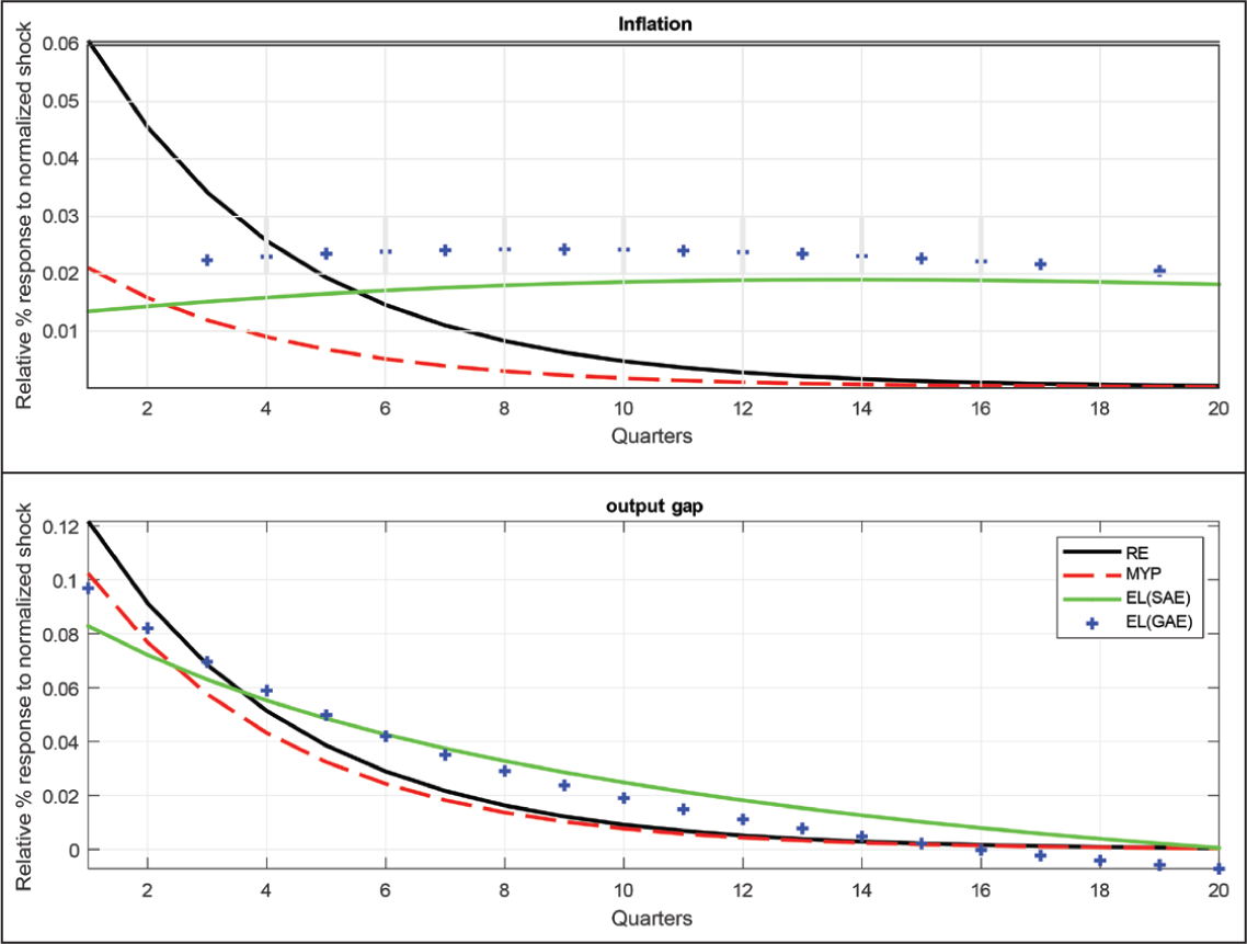
In Figures and 2 and 3, parameter values are set at their priors used later in the estimation. The demand shock follows an AR(1) process with persistence ρ_u = 0.75. These two graphs clearly illustrate the absence of robustness for the original Taylor rule, both in terms of the impulse responses to the demand shock in Figure 2 and the policy space that gives determinacy and stability in Figure 3. This clearly demonstrates the need for robust policy design across competing models (see Deák et al., 2023).

Does Imperfect Information Improve Data Fit?

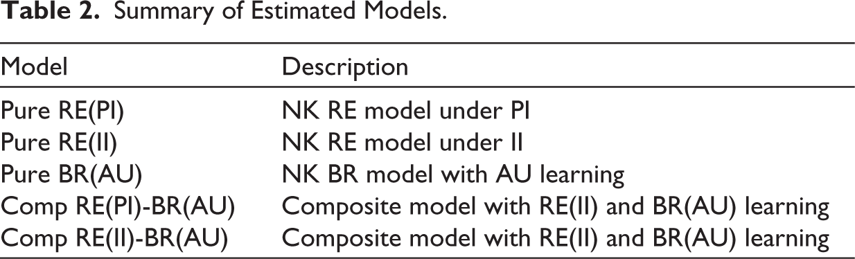
We estimate five NK models with different assumptions regarding expectations and in­formation summarized in Table 2. For the RE agents in either the ‘pure’ or composite RE–BR model, we compare the PI or II assumptions.

For each of these five models, Bayesian methods are employed to separately esti­mate the model parameters using Dynare adapted to handle II. ⁷ The sample period is 1984:1–2008:2, a subset of that used in Smets and Wouters (2007), which is also used extensively in the empirical and RBC literature. These observable variables are the log differences of the real GDP (GDP_t) and the GDP deflator (DEF_t), and the federal funds rate (FEDFUNDS_t). All series are seasonally adjusted and taken from the FRED Database available through the Federal Reserve Bank of St. Louis and the US Bureau of Labor Statistics.

We first focus on Pure RE, Pure BR(AU) and Comp RE(PI)–BR(AU) when RE agents have a PI set. We employ the Bayes factor (BF) from the model marginal likelihoods to gauge the relative merits across the three models in Table 3.

Figure 2.

Impulse Responses Comparison Between Four Log-linearized Models to a Demand Shock.

Figure 3.

Note: Green region is determinacy/stability and red region is indeterminacy or instability for EL models

Table 2.

Summary of Estimated Models.

Model	Description
Pure RE(PI)	NK RE model under PI
Pure RE(II)	NK RE model under II
Pure BR(AU)	NK BR model with AU learning
Comp RE(PI)-BR(AU)	Composite model with RE(II) and BR(AU) learning
Comp RE(II)-BR(AU)	Composite model with RE(II) and BR(AU) learning

Table 3.

Log-likelihood Values and Posterior Model Odds: RE Agents with PI.

Model	Pure RE(PI)	Pure BR(AU)	Comp RE(PI)-BR(AU)
LL	1656	1666	1672
Prob	0.0000	0.0034	0.9966

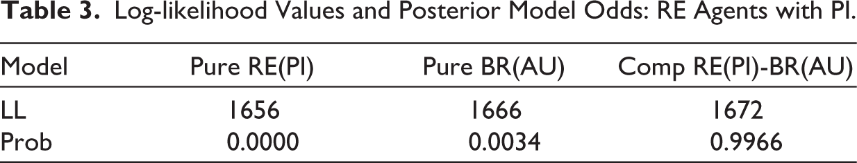
The BR models—Pure BR(AU) and Comp RE(PI)-BR(AU)—all substantially out­perform, their RE counterpart, which is firmly rejected by the data. Formally, using the Bayesian statistical language of Kass and Raftery (1995), a BF, the quotient of the prob­abilities reported, greater than 100 (marginal log-likelihood difference over 4.61), offers ‘decisive evidence’. Thus, we have decisive support for the pure BR and some composite behaviour from the US data we observe. The BF difference between the non-RE models is also strong.

Next we assume a II set for the RE agents: I_t = [Y_s−1, Π_s−1, R_n,s], s ≤ t. An important point to stress is that this is the same information set we assume for BR agents when they come to update their heuristic rule. In this sense, we now have informational consistency across BR and RE agents, and also with the econometrician estimating the model. This feature, we believe, is new for the heterogeneous behavioural NK model literature. The results for the likelihood race are reported in Table 4.

Table 4.

Log-likelihood Values and Posterior Model Odds: RE Agents with II.

Model	Pure RE(II)	Pure BR(AU)	Comp RE(II)–BR(AU)
LL	1692	1666	1708
Prob	0.0000	0.0000	1.0000

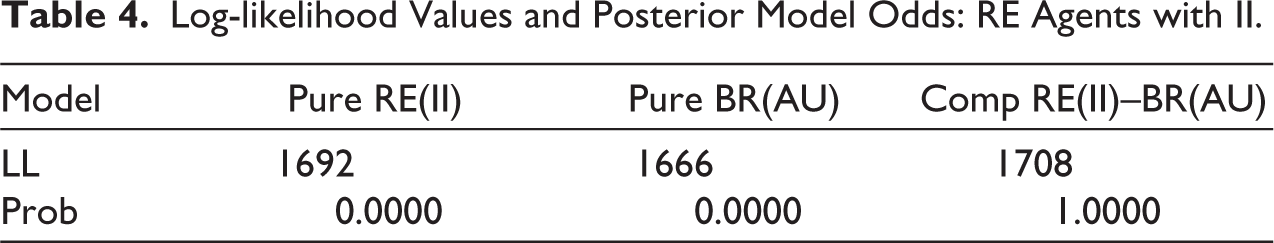
A very different picture now emerges when comparing the RE model with the be­havioural alternatives. Two results are worth noting. First, RE with imperfect informa­tion (Pure RE(II)) wins the likelihood race against both Pure BR(AU) and Pure RE(PI). Again, in formal Bayesian language, the RE(II) model decisively dominates the pure BR-AU learning model and, not surprisingly, decisively dominates RE(PI), a finding that is consistent with that in Levine et al. (2012a). The second interesting result is that, when the composite heterogenous expectations model is estimated assuming the same II infor­mation set for everyone (Comp RE(II)–BR(AU)), it generates the highest log-likelihood value and outperforms all the competing models in fitting the data.

These results suggest that persistence can be injected into the NK model to improve data fit in two contrasting ways: bounded rationality with learning through heuristic rules or retaining RE but with II and Kalman-filtering learning.

Concluding Remarks

Our results for the workhorse NK model suggest a new perspective for the macro/NK/learning literature. Avenues for future work could embed the RE–BR composite model into a richer NK model along the lines of Smets and Wouters (2007), extend the linear Kalman filter to accommodate the non-linearity in reinforcement learning and use non-linear estima­tion methods to identify a number of parameters that cannot be identified using linear Bayesian estimation. The latter two non-linear extensions are major challenges. Future work could also examine optimal monetary policy and follow Geweke and Amisano (2012) and Deák et al. (2023) to address what has been called the ‘wilderness of non-RE’ to design a robust rule across all the BR model variants discussed in the article.