
Abstract
The study develops a standard New Keynesian model to examine how monetary authority reacts to both domestic and external shocks as well as how its policy decision impacts the general macroeconomy in developing African economy. Using Bayesian estimation techniques and a Ghanaian dataset, the article also seeks to determine the best-suited monetary policy rule for Ghana and countries with similar characteristics. The basic finding is that a forward-looking Taylor rule—where authority reacts to one-period-ahead inflation deviation from target alongside the current output gap—is the most appropriate monetary policy rule for Ghana. Another salient finding is that variations in output are mainly driven by price markup, labour supply, monetary policy and productivity shocks across the forecast horizons. In addition, the dominant determinants of inflation are exchange rate risk premium and price markup shocks. Collectively, the article also unveils that monetary policy responses to macroeconomic shocks are broadly in line with conventional economic theory. There is also conspicuous evidence that the general equilibrium model with representative consumers is practically suitable for monetary policy analysis in Ghana, as contractionary monetary policy impulse is able to contemporaneously induce disinflation and output contraction. Given the strong evidence of a large segment of the unbanked population in Ghana, the findings in this study could be verified based on a model that allows for the co-existence of optimizing and non-optimizing consumers.
Keywords
Introduction
Policy transmission is one of the important areas of research for central banks, particularly in developing economies. To enhance the understanding and effectiveness of monetary policy transmission, momentous advances have been made particularly with the generation of New Keynesian (NK) models since the 1980s. These models, which combine micro-founded dynamic stochastic general equilibrium (henceforth DSGE) with the assumption of monopolistic competition and various types of nominal and real rigidities, have become increasingly popular and standard workhorse in monetary policy analysis (see Clarida et al., 1999; Goodfriend & King, 1997; Gupta & Kabundi, 2010, 2011; Ireland, 1999; Rotemberg & Woodford, 1997; Woodford, 2003). The methodological advances in NK-DSGE models 1 have provided answers to relevant policy questions in open economy macroeconomics (see Uribe & Schmitt-Grohe, 2017). For that reason, an increasing number of central banks and other large institutions, such as the International Monetary Fund (IMF), have embraced these models for the conduct of policy analysis and forecasts over the past four decades.
In this study, we develop and estimate a small open economy’s NK-DSGE model for monetary policy analysis in developing African economy using a Ghanaian dataset. 2 Specifically, the model is used to address a number of policy issues: Are monetary policy responses to macroeconomic shocks consistent with economic theory? What are the main drivers of output and inflation in the Ghanaian economy? Given the large size of the public sector and its crucial role in employment and consumption in most developing African economies, what is the impact of an increase in government spending in Ghana? Does exchange rate depreciation (or appreciation) stimulate (or dampen) economic growth and private consumption in Ghana? Are there significant spillover effects from the foreign economy to the Ghanaian economy? What is the most appropriate monetary policy rule for Ghana? The latter question is particularly motivated by the fact that most empirical studies for developing and emerging economies just either assume the standard Taylor rule or the augmented Taylor rule with exchange rate. There is, however, no clear consensus on the empirical validity of such specifications for small open developing and emerging economies 3 . In the midst of empirical indefiniteness, the current forecasting model of the Central Bank of Ghana (BOG) also utilizes a forward-looking policy rule where authority reacts to third-quarter-ahead inflation deviation from target alongside current output gap.
The model parameters in this study are estimated using Bayesian techniques with the Metropolis–Hastings (MH) algorithm, exploiting Ghana as a home economy and the Euro Area as the foreign economy. Our choice of the Euro Area as a representative foreign economy is mainly due to its sizeable share of Ghana’s external trade. The design of our small open economy model builds on previous works done in this area, notably by Smets and Wouters (2002, 2003, 2007), Gali and Monacelli (2005), Clarida et al. (2000), Christiano et al. (2005), Adolfson et al. (2007), Almeida (2009), Liu and Gupta (2007), Liu et al. (2009, 2010), etc. In line with Smets and Wouters (2002, 2003, 2007) and Erceg et al. (2000), the model exhibits sticky but forward-looking nominal price and wage settings that adjust following a staggered Calvo mechanism.
The salient empirical finding is that a forward-looking policy rule—where policy reacts to a one-quarter-ahead inflation deviation from target along with a contemporaneous output gap—is the most appropriate policy rule for Ghana. This empirical finding reinforces that the use of other policy rules (such as the standard contemporaneous rule, the backward-looking rule or the augmented rules with exchange rate or foreign interest rate) is inclined to generate less plausible estimates for policy inference in the context of Ghana. Shocks that are important for output variations are domestic price markup, labour supply, domestic monetary policy and productivity shocks. On the other hand, the dominant determinants of overall inflation are risk premium (UIP) shock and domestic price markup. Collectively, the article also reveals that monetary policy responses to macroeconomic (domestic and foreign-origin) shocks are broadly in line with conventional economic theory. There is conspicuous evidence that monetary policy shock is not prone to price puzzle, as consumer inflation falls contemporaneously following a contractionary monetary policy shock.
More importantly, the article offers a notable contribution to existing literature for Ghana and beyond. First, the Bayesian DSGE modelling is a contribution worth mentioning, as it has received very little attention in Ghana and other developing African economies. In addition, there is virtually no study that has explored Bayesian DSGE techniques for monetary policy analysis in the context of Ghana. 4 Second, the consideration of suits of monetary policy rules to determine the most appropriate rule for the Ghanaian macro-policy environment is a contribution worth noting. Third, the article extends the Ghanaian literature beyond Bayesian NK-DSGE models which could be operationalized in a policy institution such as the central bank. This is achieved by incorporating a large number of shocks into the standard small open economy DSGE model structure, following Smets and Wouters (2002, 2003, 2007). In all, we consider 11 structural shocks in this article. Specifically, there are two supply shocks (i.e., productivity shock and labour supply shock), four markup shocks (i.e., domestic price markup shock, wage markup shock, UIP shock and foreign inflation shocks), demand shocks (i.e., preference shock and foreign output shock) and three policy shocks (i.e., domestic policy shock, government spending shock and foreign policy shock). The inclusion of an expansive set of shocks is vital so as to replicate the time-series properties of the data adequately.
The article is organized such that the following section highlights the main features of the NK model adopted in this study. The third section discusses the estimation methodology and dataset employed in this study. The fourth section presents the analysis of the empirical results while the fifth section concludes and provides policy suggestions.
The Canonical Small Open Economy Model
The model in the study has two economies (home and foreign) that interact in both the goods and financial markets. The home economy is assumed to be insignificantly small in size relative to the foreign economy. Consequently, the foreign economy is assumed to be exogenous to developments in the domestic economy. The model also consists of forward-looking agents who are made up of households, firms and the government. Households maximize their expected lifetime utility by consuming goods (produced domestically and foreign imports) and supplying labour and capital to firms. Households are able to smooth consumption via habit formation in consumption. The firm, in turn, produces goods and sets prices so as to maximize expected profit. The government ensures a balanced budget at all times, spends on only consumption goods (no public investment) and sets the short-term interest rate based on a Taylor-type rule. The subsequent subsections lay out the model in stages, starting with the specification of households.
Households
The domestic economy is inhabited by a continuum of infinitely lived intertemporal optimizing households that seek to maximize their lifetime utility function given by (as in Coenen & Straub, 2005; Costa Jr., 2016; Palas, 2017; Smets & Wouters, 2002;):
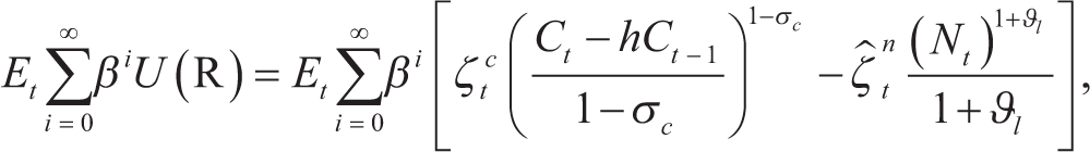
where CR,t and NR,t are consumption and labour supply of households R; vc is the intertemporal elasticity of substitution between consumption and leisure; jl is the inverse of the Frisch labour supply elasticity;

with
Each infinitely lived optimizing household, R, seeks to maximize a lifetime utility function in (1) subject to the budget constraint:

and the law of motion of capital:
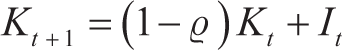
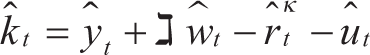
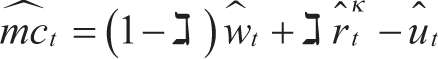
over uncertain streams of consumption (Ct), labour supply (Nt) investment (It) capital (Kt + 1) and 1-period government bonds (Bt + 1). Also, Et is the expectation operator conditional on the information set available to households at time t, Wt is the nominal wage households charge for hiring out Nt;

where
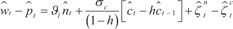
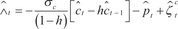
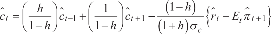
Equation (5) is the log-linearized consumption Euler equation, which determines the households’ savings decision based on comparing the utility rendered for consuming an additional amount today with the utility that would be rendered by consuming more in the future. Equation (6) indicates that the representative optimizing household equates the marginal cost of working, in consumption units, with the marginal benefit, the real wage. Equation (7) is the log-linearized Lagrangian multiplier. Equation (8) is the log-linearized law of motion of capital. The bundle of goods consumed by respective households is expressed in log terms as
Wage Determination
Each Household supplies only one type of labour, indexed
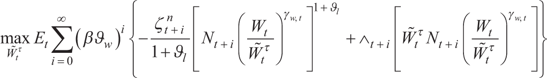
Solving the optimization problem yields an expression for optimal wage,
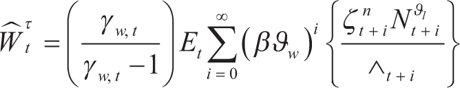
The aggregate nominal wage level for households is given by
Equation (10) indicates that the optimal nominal wage is the markup (equal to

where
The Firm
In line with the standard literature, there are two groups of firms, namely final and intermediate good producing firms. The ensuing subsections highlight the salient features of each group of firms.
The Final Good-Producing Firm
There is a competitive firm that produces the final good for consumption and investment using a continuum differentiated intermediate goods with a Dixit–Stiglitz aggregator
where Yt is a final good in period t; Yj,t for
The Intermediate-Good Producing Firm
There is a continuum of intermediate firms that operate the same technology and have identical per unit cost of production. The intermediate good producing firm, i, adopts the following Cobb–Douglas production function (in log deviation terms):
where
p℧ is the autoregressive parameter of productivity with
Firm’s profits (that are distributed to optimizing households) are expressed as
Following Calvo’s (1983) staggered price setting, only a fraction of domestic intermediate firms with probability (1 – jh) are allowed to re-optimize their price for each period. Each firm that can re-optimize its price in a given period will choose a common new price,
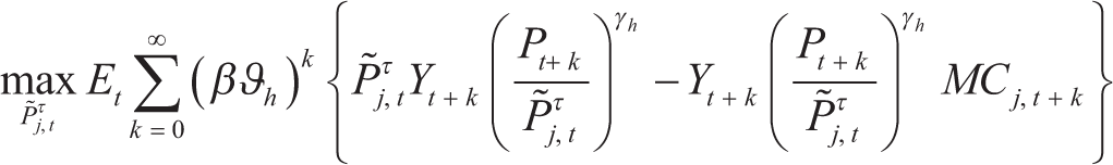
The FOC of the optimization problem yields the expression for optimal price
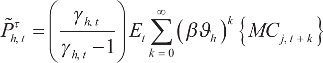
Equation (20) reveals that the optimal domestic nominal price is the markup
On the other hand, each firm that does not re-optimize its price is assumed to index its price to last period’s inflation:
Log-linearizing Equations (20) and (21) yield an expression for gross domestic inflation equations:
where
Government
As often in the NK literature, we assume a cashless economy (see Woodford, 2003). The government comprises the fiscal authority and the monetary authority. For simplicity, the fiscal authority endeavours to keep a sustainable debt-to-GDP ratio by imposing lump-sum taxes. Thus, the fiscal authority collects lump-sum taxes and also issues a one-period domestic bond (Bt) to finance the government’s spending and debt. The government budget constraint is presumed to follow the evolution that debt issuance is equal to the expenditure–revenue gap (see Baltini et al., 2009):
where Bt denotes the nominal value of a one-period government bond; Tt denotes lump-sum taxes; Gt represents the real government expenditure on the final good. For simplicity, we assume that the government only consumes goods and there is no public investment, as in Smets and Wouters (2003) and Palas (2017). Since fiscal debt clears government budget constraints, the lump-sum taxes require a separate equation that includes fiscal debt and public spending, similar to Gali et al. (2003):
where
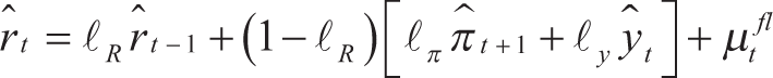
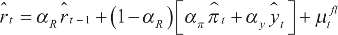
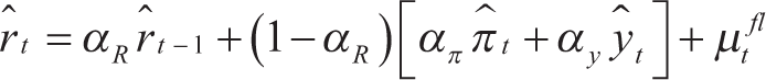
The monetary authority also controls the short-term interest rate, Rt. Monetary policy is specified in terms of an interest rate rule. In this case, monetary authority follows an augmented Taylor rule, which wields the nominal interest rate to secure the objectives of minimizing volatility in both output and expected CPI (overall) inflation. Such a reaction function also incorporates a stochastic component. Log-linearizing the interest rate rule around the steady state implies the form:
with
Foreign Economy
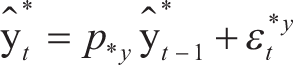
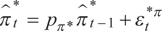
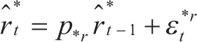
The foreign economy has a similar structure to the domestic economy. However, the domestic economy is assumed to be insignificantly small relative to the foreign economy. Consequently, the foreign economy is assumed to be exogenous to developments in the home economy. We assume that the output, inflation and policy interest rate equations for the foreign economy follow an AR(1) process (in log terms):
In addition, foreign demand for domestic goods (i.e., aggregate export demand) is expressed in log terms as
X denotes the degree of opening for the foreign economy;
International Risk Sharing and Linkages
Changes in the terms of trade represent changes in the competitiveness of the domestic economy. Assuming that the law of one price (LOOP) holds at all times, the price of domestic goods can be mathematically expressed, in log terms, as
where ft is the nominal bilateral exchange rate between the home and foreign economy, in terms of the home currency. Given Equation (31), the terms of trade, (X) which is defined as the price of foreign goods (PF, t) in terms of domestic goods (PH, t), can be expressed in log terms as
The real exchange rate is defined as the ratio of both countries’ CPI expressed in terms of the domestic currency. Since

Given the complete international financial market and a further assumption that foreign and domestic optimizing households have identical utility functions, we obtain uncovered interest rate parity (UIP), in log terms, as
where
Equilibrium Condition/Market Clearing
All goods produced by firms are consumed by households. Final home goods are partly exported

where a variable with ‘-’ denotes a steady state level. Further substituting of Equations (29) and (30) results in a log-linearized expression for equilibrium condition in the home economy yields

Empirical Methodology and Dataset
In this section, we first discuss how we estimate the structural parameters and the process governing the 11 structural shocks.
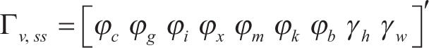
Following the extant literature (e.g., Almeida, 2009; An & Schorfheide, 2007; Rudolf & Zurlinden, 2014; Schorfheide et al., 2010, etc.), the rational expectation solution of the log-linearized model is estimated using Bayesian estimation techniques. 6 Following Almeida (2009), all parameters exclusively affecting the dynamic behaviour of the model were estimated, while parameters affecting the steady state were calibrated. The calibrated parameters are those pertaining to at least one of the following categories: (a) those parameters that are able to replicate the main steady-state key ratios of the Ghanaian economy; (b) those for which reliable estimates exist; and (c) those for which estimation was attempted but a satisfactory identification was not achieved.
Prior Distribution
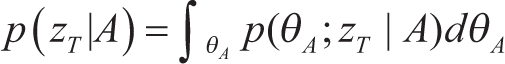
Priors are described by a density function of a form
where A stands for a specific model, iA denotes the parameter of model A, P(.) connotes a probability density function (pdf), conditional on past studies or/and occurrences or simply, reflecting subjective views of the researchers without any reference to the data. For the prior functional form, the general practice in the literature is that the inverse gamma distribution is utilized for parameters that are restricted to be positive, while beta distribution is employed for parameters that are confined to fall within 0 and 1. On the other hand, normal distribution is deployed for parameters without bounds. Amid inadequate empirical evidence, we prefer relatively diffused priors that cover a wide range of parameter values. Particularly, beta distribution is adopted for the structural parameters (such as the autoregressive shock process) that are theoretically constricted to lie between 0 and 1. In line with the literature, the inverted gamma distribution is used for the standard errors of the shock processes, as it ensures a positive variance but with a large domain.
The Likelihood
Blanchard and Khan (1980) demonstrated that linear rational expectation models can be written as a linear combination of backward-looking and forward-looking solutions. Subsequently, different approaches for solving linear rational expectation models have emerged.
7
However, the extant literature clearly articulates that the assumptions about the formation of beliefs and expectations result in a sequence of reduced-form matrices. Following the extant literature, our solution method for the version of the linear rational expectation NK model described in the second section can therefore be written as

where mt is a nx1 vector of jump and state variables (where n denotes the number of equations) and ft is a lx1 vector of exogenous variables ft is generally assumed to be white noise and to have Il as their covariance matrix. As in Binder and Pesaran (1997) and Kulish and Pagan (2014), Equation (38) can be generalized to allow additional lags of mt as well as conditional expectations at different horizons and from earlier dates. If it exists and is unique, the solution to Equation (36) will be a VAR of the form
where mt contains the endogenous state vectors; Q and G are functions of the model’s deep parameters; H expresses the link between the observed and state variables. Given the sample data,
where vt is an iid measurement error with

where
Posterior Distribution
After specifying the priors and deriving the likelihood, the posterior distribution,
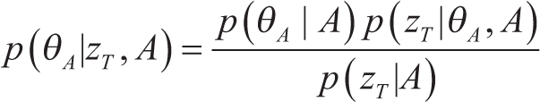
where
The numerator of Equation (42) corresponds to the posterior kernel:

The posterior kernel is the un-normalized posterior density, given that the marginal density is constant or equal for any parameter. The log-posterior kernel is expressed as
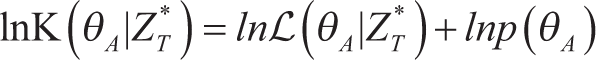
where the term on the right-hand side is known after carrying out the KF recursion, while the second terms are the priors which are also known. Thus, the mode of the posterior distribution is identified by simply maximizing the log-posterior kernel with respect to iA using the Laplace approximation. Since the distribution of the deep parameters is given by a nonlinear posterior kernel in Equation (45), direct sampling is difficult. As a result, we utilize the MH algorithm, which is a Markov Chain Monte Carlo (MCMC) method, to simulate the posterior distribution. The MH method is well-acclaimed in the literature as an efficient sampling method for obtaining a sequence of random samples from a probability distribution from which direct sampling is problematic.
The linear rational expectations NK model in the second section is solved using Dynare, a MATLAB-based software platform for handling a wide class of economic models, in particular DSGE (Griffoli, 2010). If the model is determinate (i.e., has a unique solution), Dynare finds the unique series of non-fundamental errors that keep the state variables bounded and produce the message ‘Blanchard and Khan conditions are satisfied’. In the case of indeterminacy, Dynare produces an error with a message ‘Blanchard and Khan conditions are not satisfied: indeterminacy’. According to Blanchard and Khan (1980), indeterminacy arises when the number of explosive roots is smaller than the number of non-predetermined variables.
Dataset and Preliminary Analysis
We estimate the parameters of the model and the stochastic processes governing the structural shock using six key macroeconomic variables, comprising real GDP (Y), private consumption (C), government consumption spending (G), private investment (I), consumer inflation (r) and nominal interest rate (R). The inclusion of both output and consumption in this study is consistent with Smets and Wouters (2002). In terms of sources, the datasets were obtained from the BOG, Ghana Statistical Services, the Ministry of Finance and Economic Planning, the World Bank’s African Development Indicators and the UNCTAD database.
The Bayesian estimates of the NK-DSGE model parameters are conditional on the information set:
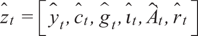
where
Since the likelihood function has to be combined with a prior density for the model parameters in order to obtain the posterior distribution of the parameters, we first discuss the choice of the prior distribution. We divide the parameters vector
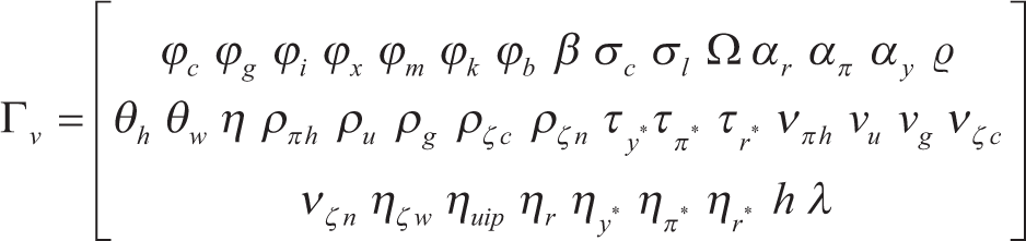
Under the Del Negro and Schorfheide (2008) prior rubic, the elements in
the parameters tied to endogenous propagation in the model

and

As a usual routine in the empirical literature, we first impose a very strict prior on a number of parameters by keeping them fixed from the beginning of this study. Most of these parameters are linked to the steady-state values of the state variables. Therefore, they could simply be derived from the means of the observed variables (or a linear combination of them). But they cannot be easily identified in the estimation procedure due to the fact that our observed variables are already demeaned. Consequently, most of the parameters in the vector

with
Columns 2–4 of Table 1 highlight the overview of our assumptions pertaining to the prior distribution of the other 29 estimated parameters. Following the extant empirical literature and to guarantee a positive variance, all the variances of the shocks are assumed to have an inverted Gamma distribution with a degree of freedom equal to 2, except for the price markup shock. However, the exact mean for the prior is determined by previous estimation outcomes and trials with a very weak prior, in line with Smets and Wouters (2002). All the autoregressive parameters for the shocks have a beta distribution with a prior mean of 0.8 and a standard error of 0.15. Although the beta distribution covers the range between 0 and 1, a rather restricted standard error is assumed so as to ensure an unambiguous disparity between persistent and non-persistent shocks.
Calibrated Parameters of the Baseline Model.
The remaining sets of parameters regarding technology, utility (or preference) and pricing settings were assumed to have either a normal or beta distribution. The means of these parameters, which are restricted within a range of 0 and 1, were set according to the extant literature. We set the corresponding standard errors to ensure that their domain encompasses a reasonable range of parameter values. With respect to the utility (preference) parameter, the prior mean for intertemporal elasticity of substitution was set to 2, consistent with Costa (2016) and close to the value used by Dagher et al. (2010) for Ghana. Similarly, the prior mean for marginal disutility of labour supply is set to 2, falling within the range of values used in the standard empirical literature. For instance, Bondzie et al. (2016) assumed a value of 1, while Dagher et al. (2010, 2012) used a value of 3 for Ghana. We, however, assumed a much wider variance of 0.75 (as in Smets & Wouters, 2002) to ensure a broader range of values. Also, the prior mean for the elasticity of substitution between home and foreign goods was set to 2. Following the empirical literature (notably, Costa, 2016; Smets & Wouters, 2002; Gali et al., 2001), the means of the Calvo parameters in the price and wage setting equations were set to 0.75. These prior values were mainly to ensure that the wage contract lasted about one year. The standard errors for the Calvo parameters were set at 0.05, mainly to allow for divergence between 3 quarters and 2 years. Besides, the discount factor, b, is calibrated to be 0.983, which implies an annual steady-state real interest rate of 7.8% (a mean long-run value for 2015–2018).
Regarding other technological parameters, we set the share of capital in production, m, to 0.3 which is in line with standard literature (notably Dagher et al., 2012). This roughly implies a steady state share of labour income in total output of 70%. We assume a prior mean of 0.7 for the consumption habit parameter, h, and a standard error of 0.2. The values were derived as the mean and the corresponding standard deviation from three detrending approaches (quadratic detrending, HP and first difference methods). The prior mean for h is within the empirical estimates by Guerron-Quintana and Nason (2012) and Kirchner and Tranamil (2016).
Finally, the prior mean for the coefficients in the monetary policy reaction function is standard. For instance, the prior mean for interest rate sensitivity to expected inflation deviation from its steady state, ar, is set at 1.4 with a standard error of 0.25. The imposition of a relatively higher ar is to obey the Taylor Principle that the interest rate rises more than the increase in inflation deviation from the target level (or steady-state value). Thus, the prior on ar is to guarantee a unique solution path when solving the model. Likewise, the prior mean for the autoregressive parameter was set to 0.8 with a standard error of 0.15. On the other hand, the parameter for policy interest rate sensitivity to current output deviation from its steady-state has a prior mean of 0.125 and a standard error of 0.35. This is based on the empirical estimates of interest rate rules that generally place ay between 0.1 and 0.5 for less developed countries (see Airaudo et al., 2016). This implies a smaller response of the policy interest rate to the output gap, but this response is non-zero.
Empirical Analysis
Here, we present the main estimation results. In this case, we deliberate on the posterior estimates after determining the most appropriate monetary policy reaction. Finally, we evaluate both the static and historical variance decomposition of shocks as well as the simulated impulse response functions (IRFs).
Analysis of the Posterior Estimates
To avoid the problem of stochastic singularity in the case where there are more observed variables than the number of shocks, more shocks were included in this analysis. Also various convergence statistics were computed. We carried out MCMC simulations with the MH algorithm using five parallel block chains for (a) 100,000 draws and (b) 300,000 draws. In this study, the empirical analysis is based on a full sample period (2000:2–2017:4), while the preceding period (2000:2–2007:1) is utilized as a training (in-sample) sample. Given the data and the prior specification in Table 1, we find almost an identical posterior distribution for two MCMC draws. For brevity, however, we report the posterior distribution generated from the five parallel block chains with 300,000 draws of the MCMC simulations. Table A1 clearly shows no significant convergence problems after 300,000 iterations. Therefore, we can generalize that all the parameters successfully converge.
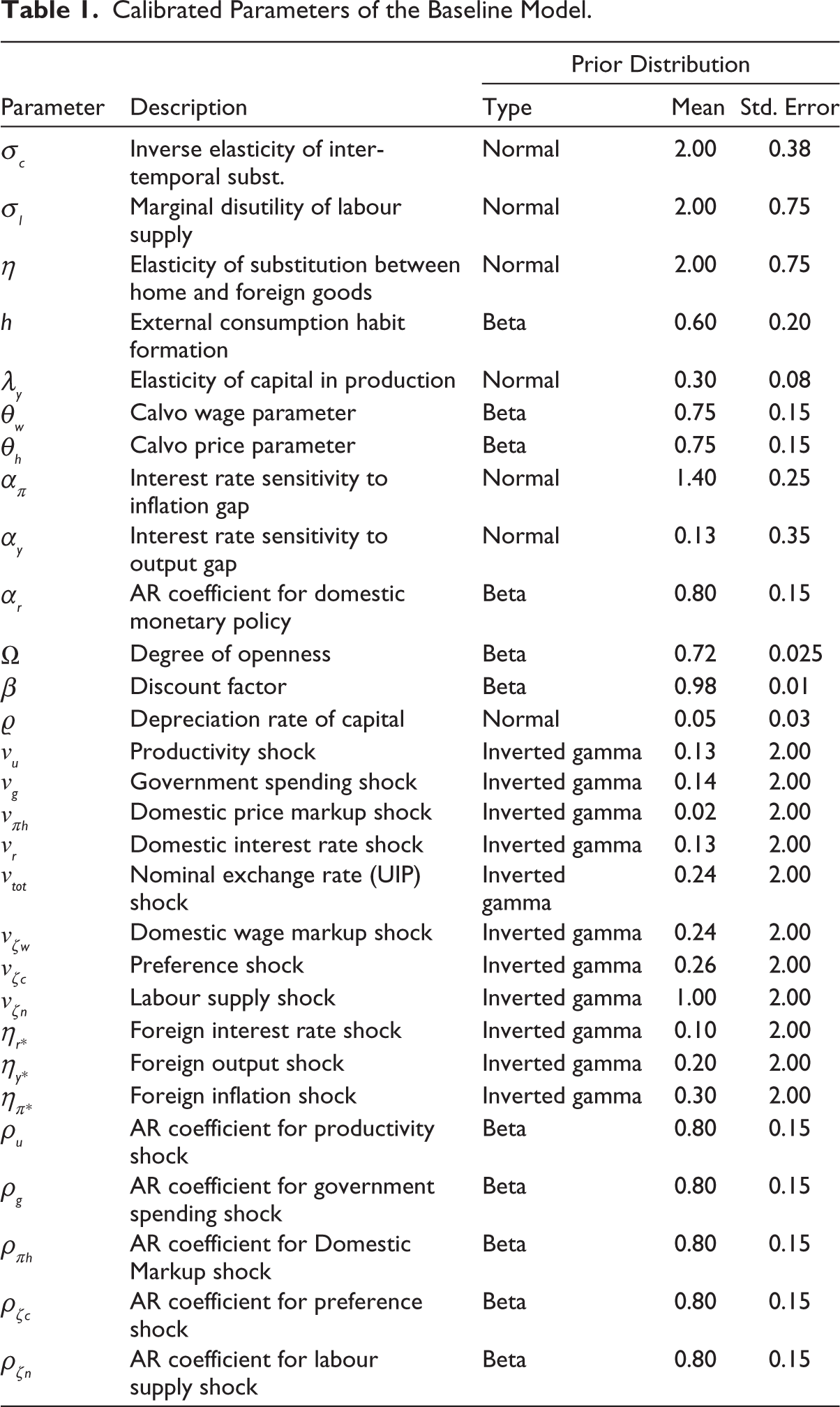
Table 2 presents two sets of posterior parameter estimates. The first category is the estimated posterior mode of the parameters with corresponding standard errors. The posterior modes are attained by maximizing the log of the posterior distribution with respect to the parameters and an approximate standard error based on the corresponding Hessian. The second category reports the estimated posterior mean with the corresponding 5% and 95% credible intervals of the posterior distribution of the parameters. The Panel A of Table 2 gives the estimated posterior distribution of the shock processes. A number of observations are worth making regarding the estimated processes for the exogenous shock variables. The posteriors for all the shock parameters are quite distinct from the assumed priors, indicating that the estimates draw important information from the data. On a whole, it appears that data are quite informative on the stochastic processes for the exogenous disturbances, as indicated by the lower variance of the posterior distribution relative to the prior distribution. The government consumption, labour supply and preference shock processes are estimated to be the most persistent, with AR(1) coefficients of 0.985, 0.945 and 0.936, respectively. In contrast, productivity is the least persistent parameter, with an AR(1) coefficient of 0.571. The mean of the standard error of government consumption is 3.394.
Turning to the estimates of the main behavioural parameters, as in Panel B of Table 2, it turns out that the mean of the posterior distribution is generally relatively close to the mean of the prior assumptions. Overall, it appears that the data are quite informative on the behavioural parameters, as reflected by the lower variance of the posterior distribution relative to the prior distribution. There are, however, few notable exceptions. The estimated posterior variances of the intertemporal elasticity of substitution, degree of openness, marginal disutility of labour and depreciation rate on capital are higher than that of the prior distribution, while the variance for capital share in production is the same for the posterior and prior distributions.
Prior and Posterior Distribution from the Baseline RANK-DSGE Model.
The external consumption habit stock, h, is estimated at 0.32, which is smaller than our prior mean and also below the estimates reported in Smets and Wouters (2002), Christiano et al. (2005) and Liu (2006). The relatively lower value for h is perhaps driven by our assumption of homogeneous optimizing households, even though the literature seems to suggest the presence of the sizeable number of hand-to-mouth consumers in Ghana (see Dagher et al., 2012). The posterior mean estimate of the intertemporal elasticity of substitution is less than 1 (vc = 0.739) and below the assumed prior distribution. Nevertheless, our estimate falls within the assumption made in much of the RBC literature, which assumes an elasticity of substitution between 0.5 and 1. It should however be noted that our model assumes an external habit formation, h, which turns out to be significant and hence, such comparison ought to be done with caution. The relatively moderate value for vc implies that households are less willing to accept deviations from a uniform pattern of consumption over time. Ignoring the preference shocks, our consumption function in Equation (5) can be written as
Given Equation (50) and our estimates for v and h, an expected 1% rise in short-term real interest rate for four quarters has an impact on consumption of about 0.697. In contrast, the estimated inverse elasticity of substitution for labour, vl, turns out be much greater than unity (vl 3.835), in line with the estimate for New Zealand as reported in Liu (2006). This implies that a 1% increase in the real wage will result in only a small change in labour supply.
The estimated posterior mean for elasticity of substitution between home and foreign goods, h, is 0.846, below the prior mean and the value used in Dagher et al. (2012) for Ghana. The relatively low value for h is broadly coherent with the fact that Ghana is a commodity-producer and foreign-produced goods form a sizeable proportion of its consumption basket. Consistently, the posterior mean for the parameter characterizing the degree of openness, X, is estimated at 0.687. Although it is slightly smaller than the assumed prior distribution, the estimates surmise that the Ghanaian economy is very open, exposing the economy to the vagaries of external developments.
There is, however, a considerable degree of Calvo price and wage rigidities. The posterior estimate for the proportion of firms that do not re-optimize their price in a given quarter is 0.73, surmising an average duration of price contracts of about four quarters (one year). In contrast, the proportion of households that do not re-optimize their wage in a given quarter is estimated at 0.70, epitomizing an average duration of wage contracts of about three quarters.
The posterior mean for the discount factor, b, is estimated at 0.979 (with a range of 0.955–0.990), which is slightly smaller than the prior mean. This implies an annual steady state real interest rate of 7.6%. The depreciation rate, u, is estimated at 0.06, implying an annual depreciation on capital of about 24%. Although this value appears to be very high, our prior mean is more informative than much of the other empirical studies. The posterior mean parameter for capital share in production, my, is found to be 0.301, nearly consistent with the prior mean. This suggests that about 70% of the production process entails labour inputs with the residual 30% contributed by capital inputs. This observation is perhaps very intuitive as the production and economic activities or set-ups in Ghana (like other developing economies) are generally labour-intensive.
Turning to the monetary policy reaction function parameters, the posterior mean parameter for interest elasticity to inflation, ar, is estimated to be relatively high (1.704) with a 95% credible range of (1.00–1.88). This illustrates that the value for ar satisfies the so-called Taylor Principles as it is greater than one and close to values suggested by Taylor (1993). There is a considerable degree of interest rate smoothing, as the mean of the coefficient of the lagged interest rate, ar, is estimated to be 0.83 with a 95% credible range of (0.77–0.88). Finally, the response to output gap, ay, is estimated to be 0.605, higher than the prior distribution and exceeding the empirical range for less developed countries between 0.1 and 0.5. It also indicates a pursuit of a flexible inflation-targeting regime in Ghana, as the standard deviation of the output gap significantly differs from zero.
Determining the Suitable Monetary Policy Rule
We then determine the appropriate monetary policy rule for a shock-prone Ghanaian economy. This is motivated by the inconclusiveness of the theoretical and empirical literature regarding the accurate specification of monetary policy rule especially for developing and emerging economies.
9
In view of this controversy, our baseline model adopts a forward-looking rule of the kind proposed by Taylor (1993), in which the monetary authority uses the nominal interest rate to secure the objectives of minimizing volatility in the current output gap and the one-period-ahead expected inflation gap. For robustness, however, we ascertain the suitability of such policy specifications for Ghana by first comparing the baseline policy rule against (a) the contemporaneous rule following Carlstrom et al. (2006) and Airaudo et al. (2016) and (b) ‘backward-looking’ rule following Smets and Wouters (2003). Explicitly, the contemporaneous and ‘backward-looking’ policy rules in this study are specified respectively as
and
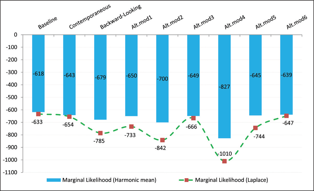
As highlighted in the extant literature, one advantage of the Bayesian estimation approach is that it provides a framework for comparing and choosing between fundamentally mis-specified models. 10 In addition, the marginal likelihood can be interpreted as a summary statistic for the model’s out-of-sample prediction performance and therefore forms a natural benchmark for comparing the DSGE model with other alternative specifications and other statistical models (see Geweke, 1999; Landon-Lane, 1998; Smets & Wouters, 2002). The identical treatments of the datasets and the prior distribution across models in our study also make the marginal likelihood estimate a suitable indicator for assessing relative model performance. On one hand, Geweke (1999) proposes the modified harmonic mean estimator (henceforth, MHM) that works for all sampling techniques to calculate the marginal likelihood necessary to compare models. On the other hand, Schorfheide (1999) calculates the marginal likelihood using a Laplace approximation method (henceforth LT) that does not depend on any sampling method but starts from the evaluation in the mode of the posterior. Thus, the latter method utilizes a standard correction to the posterior evaluation at the posterior mode to approximate the marginal likelihood. Although both estimators (LT and MHM) are employed in this study, the preferred statistic is the MHM estimator, as it is argued to be insensitive to step size (Smet & Wouters, 2002).
Figure 1 presents the marginal likelihoods of the alternative models, given the dataset and prior distribution. The figure reveals that the model with either a contemporaneous or backward-looking rule yields a lower marginal likelihood compared with the baseline model with a forward-looking rule. This empirical evidence is unanimous from both LT and MHM estimators. By implication, the baseline model with forward-looking rules appears to fit the Ghanaian macroeconomic datasets much better than the DSGE model with either contemporaneous or backward-looking policy rules.
Second, we compare the out-of-sample forecast performance of the baseline model against alternative models with augmented forward-looking or contemporaneous policy rules. In this case, we incorporate the exchange rate or/and foreign interest rate to basically account for the increasing role of the exchange rate in developing economies and also the pace of global financial integration, respectively. In all cases, as illustrated by Alt.mod1–4 in Figure 1, the alternative specifications deteriorate the marginal likelihood when compared to the baseline model. Subsequent to this realization, the third exploration is to determine how far into the future the monetary authority in Ghana should consider regarding expected inflation deviation from target within its forward-looking policy rule. This is motivated by the fact that the current FPAS model of BOG utilizes a policy rule with a third-quarter-ahead inflation gap alongside the current output gap. In view of that, we ascertain the relative out-of-sample prediction performance of the baseline rule against alternative flexible rules where authority reacts to (a) second-quarter-ahead (t+2) and (b) third-quarter-ahead (t+3) inflation deviation from target alongside the output gap. Alt.mod5 and Alt.mod6 in Figure 1 report the marginal likelihoods for specifications (a) and (b), respectively. Similarly, it is obvious from Figure 1 that the baseline rule generates a higher marginal likelihood compared to both cases (a) and (b), indicating a relatively better fit from the baseline rule.
where
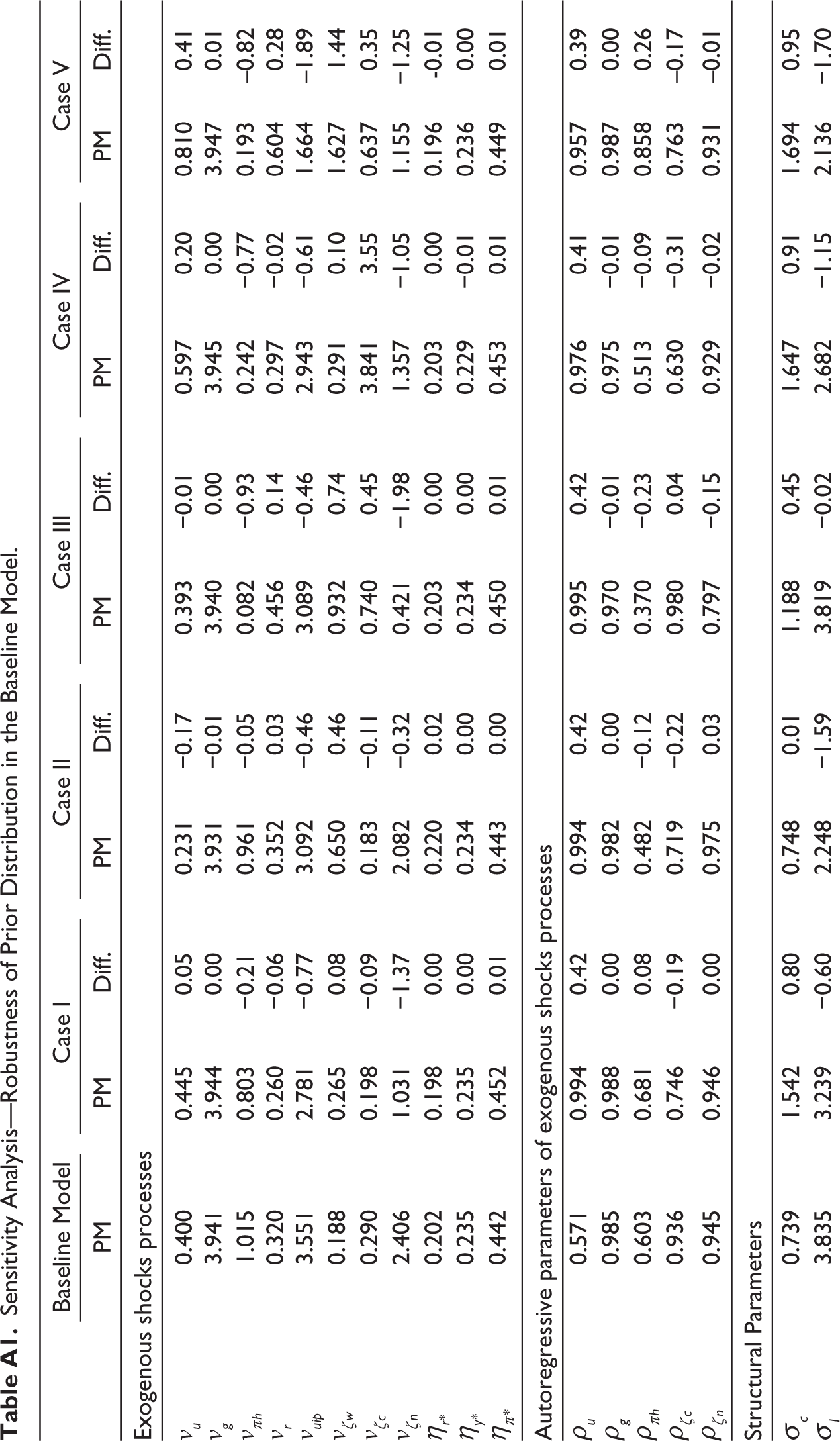
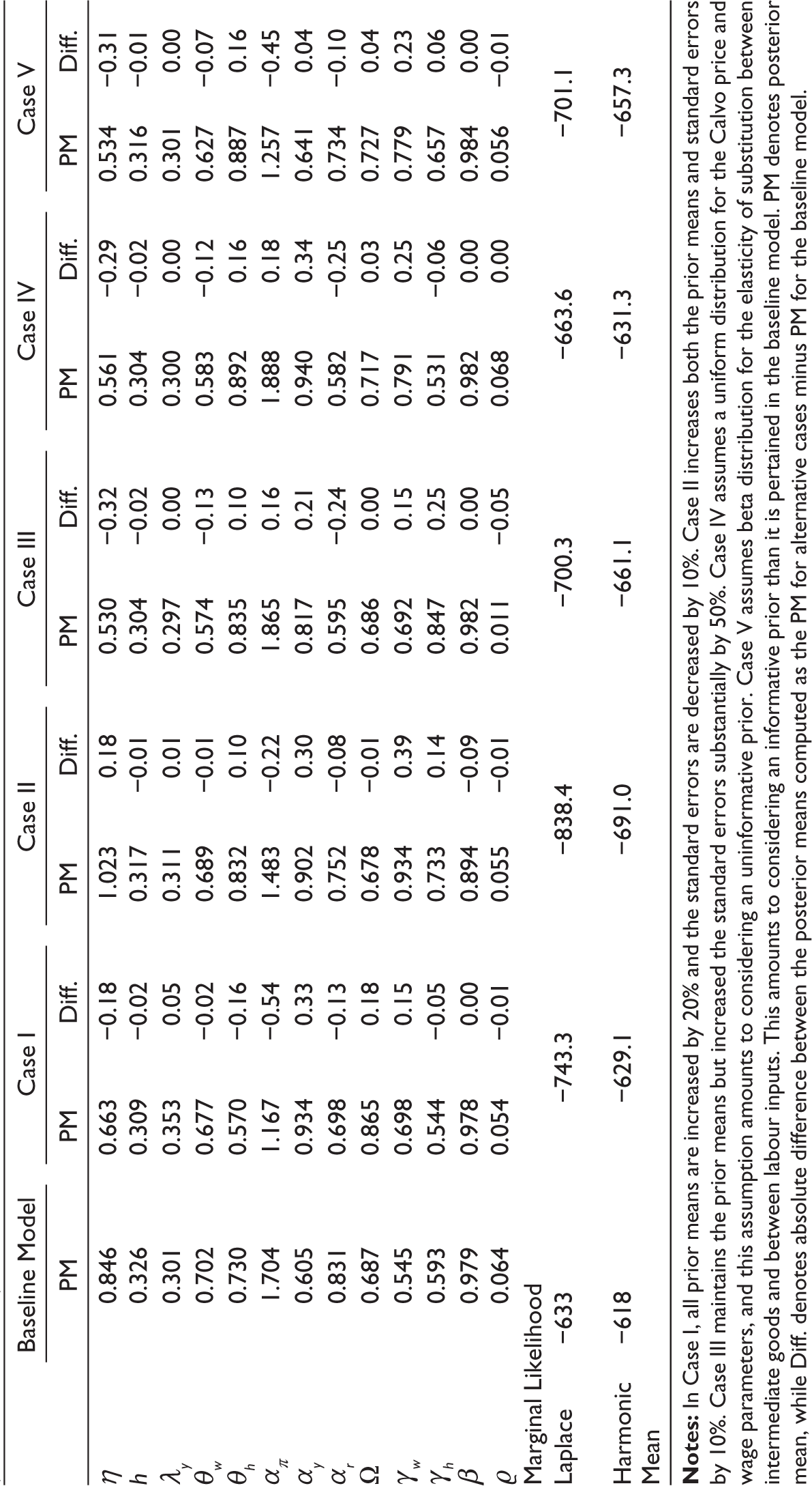
Conspicuously, the baseline model provides much better out-of- sample prediction performance of the Ghanaian macroeconomic data than all the alternative models considered. By implication, the study reveals that forward-looking monetary policy rule—where authority reacts to one-period-ahead inflation deviation from target and current output gap—is the most appropriate policy rule for the Ghanaian dataset considered. The second-best policy rule detected in this study is the forward-looking policy rule with a three-quarters-ahead inflation deviation from target and current output gap. The empirical observation contradicts the assertion by Airaudo et al. (2016), and therefore the advocates by Carlstrom et al. (2006) cannot be generalized to the open economy model. It also connotes that studies that adopt either the contemporaneous or backward-looking rule may yield less plausible posterior estimates for policy inferences in Ghana, and by extension, developing economies with similar characteristics. Furthermore, our sensitivity analysis reveals a more robust prior distribution of the baseline model (see Table A1 in Appendix A) as each of the alternative scenarios results in considerable deterioration in marginal likelihood relative to the baseline.
Analysis of Structural Shocks: Static and Historical Contributions
Table 3 presents the relative average contribution of each of the structural shocks to the forecast error variance of the endogenous variables at various horizons. In this section, we consider 11 structural shocks. They are two supply shocks (i.e., productivity shock and labour supply shock), four markup shocks (i.e., domestic price markup shock, wage markup shock, UIP shock and foreign inflation shocks), demand shocks (i.e., preference shock and foreign output shock) and three policy shocks (i.e., domestic policy shocks, government spending shock and foreign policy shock).
Forecast Error Variance Decomposition (%).
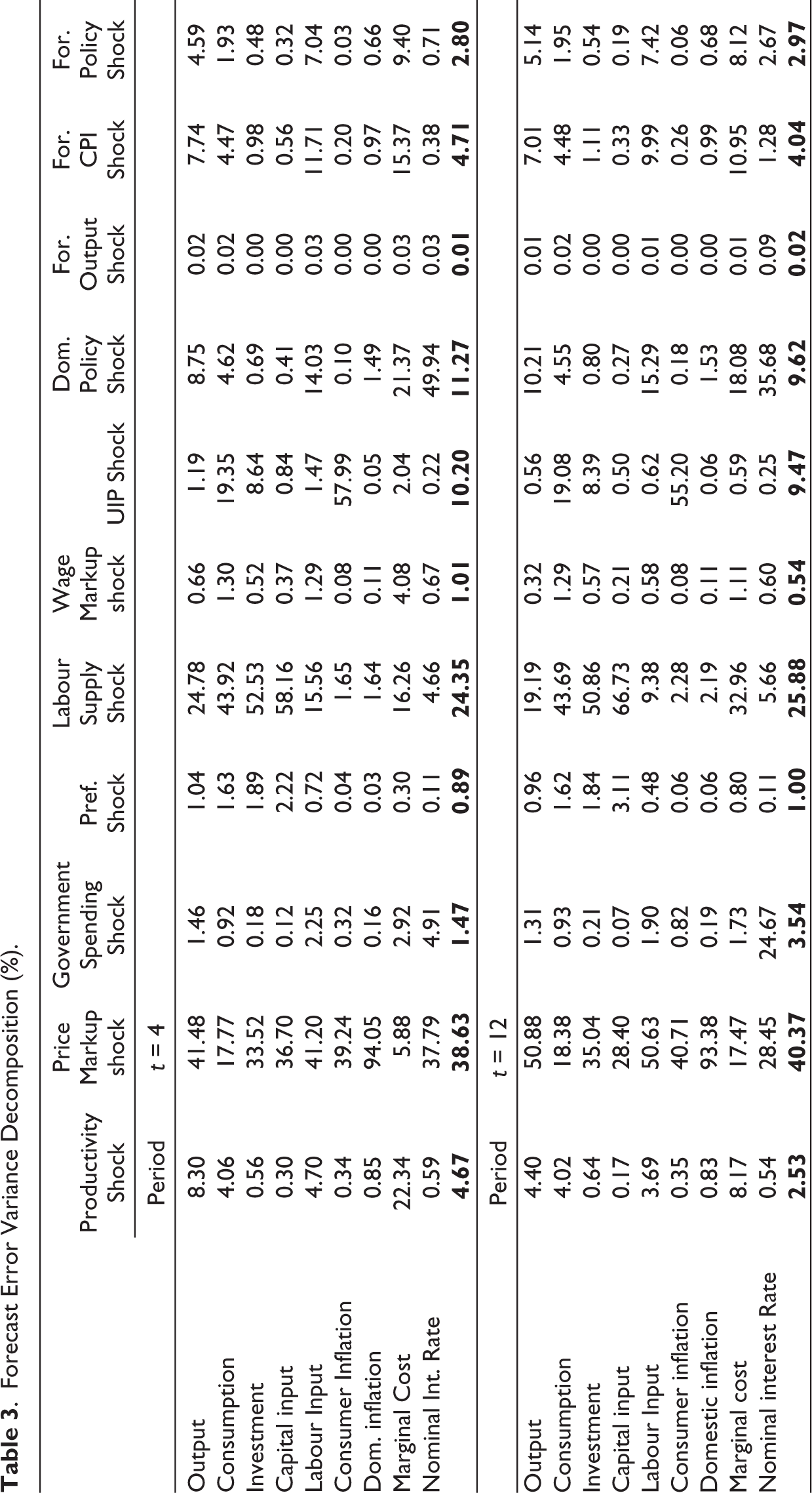
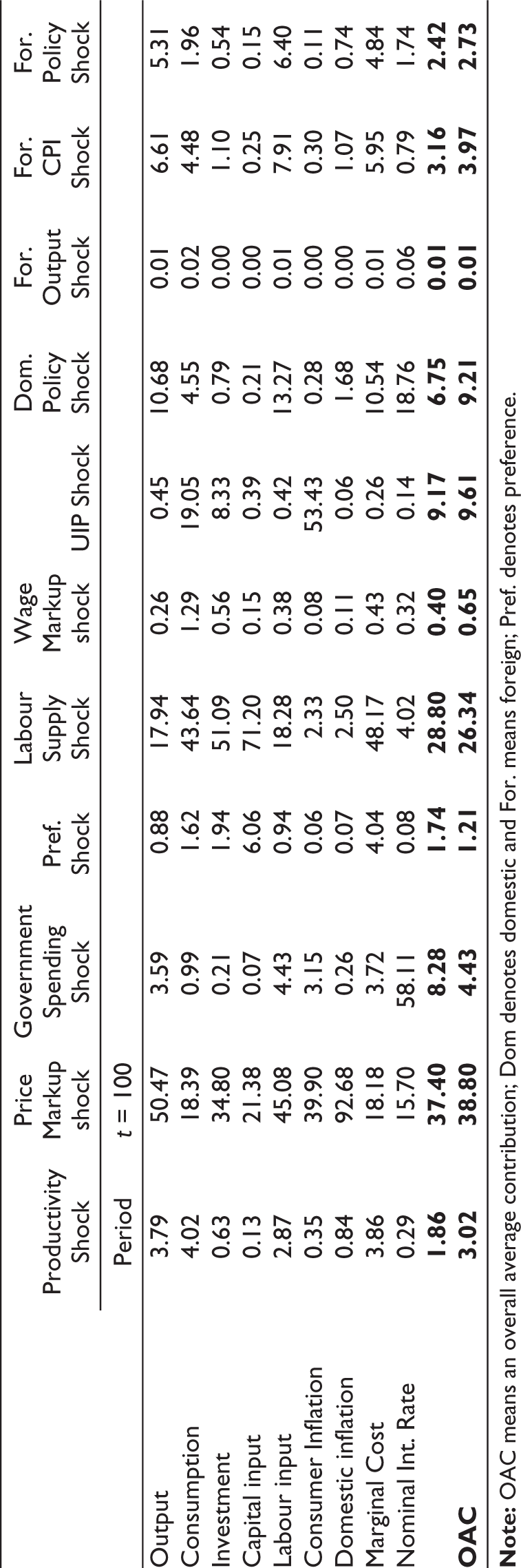
Starting with output dynamics, we find the dominant drivers (in descending order) to be price markup shock, labour supply shock, domestic monetary policy shock, productivity shock, foreign inflation shock and foreign policy shock across the forecast horizon (i.e., short–medium–long run). Notably, the table reveals that productivity shock has a limited average influence on aggregate fluctuation in Ghana, while domestic monetary policy matters for economic growth. The average contribution of domestic monetary policy shock to variations in output is primarily via its implication on the cost of labour and capital inputs. In the case of consumer inflation (CPI), the main determinants are exchange rate risk premium (UIP) shock and domestic price markup shock. The predominant influence of UIP shock on the variations in CPI inflation is largely driven by the estimated high degree of openness in Ghana. This also suggests that the exchange rate is a leading conduit for the volatility spillovers from the foreign economy. Concerning monetary policy function, the dominant determinants of the nominal interest rate in the short-term horizon are domestic monetary policy, price markup shocks, government spending shock and labour supply shock. This observation surmises that the continuous large fiscal overruns have a considerable debilitating impact on the monetary policy stabilization effort in Ghana.
The preceding analysis focuses on the average (or static) contribution of shocks to the variations in the key macroeconomic variables. It, however, does not highlight the time-varying or historical contribution of shocks which is essential for the interpretation of the historical evolution of these variables. In addition, the averaging method may possibly mask the salient periodic contributions of some structural shocks over the entire spectrum of the interested macroeconomic variable. Consequently, we further explore the historical (time-varying) contribution of shocks to inflation and output gap by utilizing the Kalman filter (KF), given the state space representations and the parameter estimates of the model. The analysis of historical shock decomposition may bring to light the model’s interpretation of chronological developments in these variables.
Figure A2 in Appendix A displays the historical shock decomposition of economic growth for the period 2006–2017. A thorough examination of the model’s estimate reveals that developments surrounding the productivity shock predominantly influenced Ghana’s GDP growth for the 12-year period. This seems to suggest that productivity shock remains an important driver of GDP gap despite its relatively smaller value in the preceding static analysis. For instance, the below-trend GDP growth from 2006 to mid-2007 was instigated by waning technological gains supported by adverse supply shock and stronger domestic currency (implying a reduction in the risk premium shock). The model estimates also suggest that the strong recovery in economic activities from mid-2007 to the third quarter of 2008 was driven by strong technological improvement in tandem with favourable international developments that outstripped adverse supply shocks. Throughout these periods, labour supply shocks also provided upward pressures on the output gap. The significant technological gain is mainly driven by the substantial infrastructural developments towards the hosting of the African Cup of Nations (AFCON) in 2008 and the Golden Jubilee celebration in 2007. On the other hand, the below-trend growth of GDP from the late 2008 to early 2009 is attributed to a decline in productivity, weaker aggregate demand and adverse supply shocks, broadly activated by the onset of the global financial crisis in late 2008. However, the model accredited the subsequent above-trend growth of Ghanaian GDP for the period between mid-2009 and early 2013 (except for 2010:1) to robust technological gains and a supportive monetary policy environment, which more than countered the adverse supply, risk premium and foreign shocks.
Additionally, labour supply shocks contributed negatively and positively to growth during the periods 2009:3–2010:2 and 2010:3–2013:1, respectively. It seems also reasonable that the favourable impact of the onset of Ghana’s crude oil production and exports in 2011 on GDP growth becomes apparent in the model’s estimates. Moreover, a decline in productivity and an adverse labour supply shock rendered a downward pressure on the output gap between mid-2013 and the third quarter of 2016. During this period, demand shock placed downward pressure on GDP growth (except in the year 2014 when it had a positive influence). It is apparent that the risk premium shock exerted a positive effect on GDP growth during this period (expect for the year 2013), reflecting the impact of the huge exchange rate depreciation experienced between 2014 and 2015. Furthermore, the subsequent above-trend GDP growth is further attributed to productivity changes, supported by favourable supply shocks and expansionary monetary policy shocks. The model’s estimates also reveal that foreign-related shocks have exerted downward pressure on Ghana’s GDP growth since 2010.
The historical shock decomposition of consumer (CPI) inflation in Figure A3 in Appendix A highlights the main shocks that contributed to inflation’s deviation from the steady state for the period 2006–2017. In the context of the model, the general drop in consumer inflation from 2006 to mid-2007 is ascribed to a considerable reduction in risk premium shock, which led to cedi appreciation. This together with favourable supply-side shocks exuded disinflationary pressures during the era. The surge in consumer inflation from mid-2007 to mid-2009 is attributed to an unfavourable supply-side shock and an escalating exchange rate risk premium. The rise in adverse supply-side shocks is partly driven by rising international commodity prices (particularly oil prices) and the resultant increase in domestic fuel prices over the period.
Conversely, the onset of the global financial crisis in late 2008 led to financial (particularly portfolio) outflow which heightened exchange rate risk premium and, hence, induced significant cedi depreciation. The drop in consumer inflation from late 2009 through to the first quarter of 2012 is attributed to a fall in international commodity prices (oil prices), a lower risk premium (linked to oil production and exports in 2011) and favourable supply-side shocks. Throughout these periods, labour supply shock has exerted downward pressure on consumer inflation, except the year 2009. The subsequent upsurge in consumer inflation from mid-2012 to mid-2016 is associated with adverse supply-side shocks and an escalating risk premium (leading to rapid cedi depreciation). As well, the labour supply shock broadly induced upward pressure on inflation during the period. Consumer inflation has fallen since late 2016 as the cedi strengthened considerably on the back of a lower risk premium as well as favourable supply-side and labour supply shocks. The lower risk premium for the period was boosted by enhanced investor confidence following a smooth transition to a political regime in 2017.
Model Dynamics: Impulse Response Functions (IRFs)
In order to analyse the dynamic reaction of the preferred baseline model in response to shocks, we discuss the impact of a selected number of structural shocks of domestic and foreign origins. The graphs plot the mean response together with the 5th and 95th percentiles.
Domestic Shocks
We begin this section by examining the macroeconomic responses to shocks originating from the domestic economy, in order to understand, especially, how the monetary authority reacts to these disturbances.
Increase in Productivity
Figure B1 in Appendix B shows impulse responses associated with an unanticipated increase in production technology. The posterior estimate for the size of the shock is 0.40 and is set to be moderately persistent with pg = 0.571. Output increases in response to improvement in production technology. Consistent with standard new-Keynesian models (see Galı, 1999, 2008; Smets & Wouters, 2002), firms cut back on labour demand (i.e., rise in unemployment), causing both the nominal wage and labour supply to plummet as production technology improves. The rise in unemployment alongside plummeting marginal costs (as costs of inputs—wage and rental rate of capital—fall) contemporaneously induces a decline in both domestic and aggregate prices. This is intuitive as less (more) inflation is the opportunity cost of lower (higher) unemployment. Consequently, the monetary authority lowers the nominal interest rate (albeit moderately) in response to the fall in prices (inflation) and higher unemployment. The expansionary monetary policy stance induces real exchange rate depreciation and a concomitant improvement in terms-of-trade. The subsequent gradual strengthening of the domestic currency alongside steady weakening terms-of-trade drives output towards its steady state level after 10 periods.
Increase in Government Spending
Figure B2 in Appendix B displays an impulse response linked to an unanticipated increase in government (consumption) spending. The posterior estimate for the size of the shock is 3.941 and is set to be highly persistent with pg = 0.985. Aggregate output increases in response to an increased government spending shock. Firms respond by increasing demand for both capital and labour (employment) inputs in order to meet the rising demand for output, resulting in a higher nominal wage and cost of capital (rent). Marginal cost increases as costs of inputs (wage and rental rate of capital) rise. Inflation increases as firms pass on the higher marginal cost into prices. In response to rising inflation, monetary authority raises the nominal interest rate. The rise in the interest rate boosts private investment, dampens aggregate household consumption and strengthens the local currency. Consistent with economic theory, the gain in the domestic currency induces negative net exports, reinforcing a subsequent drop in output towards its steady level. In the context of Ghana, we observe a net crowding-out effect of the expansionary fiscal policy on household consumption. In line with the permanent income hypothesis, households seem to save or invest the transitory income emanating from government spending amid concerns about fiscal solvency in the long run.
Contractionary Domestic Monetary Policy
Figure B3 in Appendix B presents the effect of domestic monetary policy contraction (i.e., positive interest rate shock). The posterior estimate for the size of the shock is 0.32. Because there is no autoregressive structure associated with shock, the gradual receding of the shock to its steady state level is mainly driven by the interest rate smoothing but not via the persistence of the shock itself. Consistently, the unexpected contractionary monetary policy leads to a rise in short-run interest rates (both nominal and real). The real exchange rate appreciates on the back of a positive real interest rate. A stronger domestic currency contemporaneously deteriorates net exports. Output declines as a result of negative net exports, causing firms to curtail employment (i.e., higher unemployment). The decline in costs of labour inputs shrinks marginal cost and, hence, induces a fall in domestic inflation. The appreciation in the domestic currency raises households’ net worth to boost private consumption, especially of imported goods, and this is facilitated by the estimated high degree of trade openness (X = 0.687). The qualitative result implies that a high degree of openness considerably impairs the effectiveness of monetary policy to restrain private consumption. Although contractionary monetary policy shock generates a decline in output and domestic inflation, which is consistent with economic theory, it rather causes overall inflation to inch up contemporaneously. This suggests that the NK model with representative agent is not able to resolve the problem of the price puzzle for the Ghanaian macroeconomy.
Labour Market Shocks
We further examine macro-responses to shocks originating in the labour market. Following the extant DSGE literature (e.g., Smet and Wouters, 2003, 2007; Chari et al., 2009; etc.), these labour market shocks could either be interpreted as an efficient shock to preference or as an inefficient wage markup shock. This exercise is motivated by the high unemployment situation in Ghana. In addition, Foroni et al., (2018) found labour supply shocks to be the main drivers of labour participation rate, unemployment rate and output growth in the aftermath of the Great Recession. Accordingly, we first report the impulse responses of a positive (favourable) preference shock to labour supply, which conceivably reflects a greater household’s willingness to work (i.e., high labour participation) and high unemployment if firms are unable to take up all the active labour force, in line with Foroni et al. (2018). Figure B4 in Appendix B displays the qualitative responses to a favourable labour supply preference shock which is assumed to exhibit an autoregressive process in line with Smet and Wouters (2003, 2007) and Foroni et al. (2018). The posterior estimate for the size of the favourable labour supply preference shock is 2.406 and is set to be very persistent with tgn = 0.945. Labour supply and output increase following a favourable preference shock to labour supply, in line with Foroni et al. (2018). The growth in output induces firms to raise investment, and their demand for capital inputs also increases. Nominal wage, marginal costs and consumption decline promptly as household’s marginal utility of work increases, leading to a slowdown in both domestic and aggregate prices. Monetary authority lowers the nominal interest rate in response to a fall in prices, leading to real exchange rate depreciation and a resultant improvement in terms-of-trade. The subsequent gradual tightening of the monetary policy stance and a steady strengthening of the domestic currency in real terms worsen the terms-of-trade, which in turn lowers output, investment and labour supply towards their steady state levels after 10 periods.
Figure B5 in Appendix B also depicts impulse responses from a positive wage markup shock (i.e., shock that increases the nominal wage). The posterior estimate for the size of the shock is 0.188 and is assumed to have no autoregressive structure, following Smets and Wouters (2002, 2007) and Chari et al. (2009). Nominal and real wages increase on impact, leading to instantaneous rise in labour supply as household’s willingness to work increases. Marginal cost increases as the nominal wage rises. This, together with an increased household consumption, causes prices to rise. Monetary policy immediately responds to the inflationary pressures by raising the nominal interest rate. The real interest rate increases in effect which in turn causes the real exchange rate to appreciate. Net export worsens due to currency appreciation (in real terms), consistent with economic theory as imports become cheaper relative to exports. Output, however, increases on impact of the positive wage markup shock as the pickup in private consumption seems to outweigh the combined drops in investment and net exports.
Foreign Spillovers
We now turn to illustrate the macroeconomic responses to shocks originating from the foreign economy in order to understand, especially, how the monetary authority reacts to foreign spillovers.
Contractionary Foreign Monetary Policy
Figure B6 in Appendix B illustrates impulse responses associated with unanticipated foreign monetary policy contraction (rate hike). The posterior estimate for the magnitude of the shock is 0.202, with no autoregressive structure. From Figure B6, it is observed that domestic currency depreciates on the impact of foreign monetary policy contraction, boosting net export and output. The rise in aggregate output induces firms to increase demand for factors of production, which in turn raises the cost of factor inputs and, hence, a surge in marginal cost. Inflation increases on the back of rising marginal costs. Overall, private consumption declines as depreciated local currency reduces the net worth of households. This is underpinned by the decline in imports (via improved trade competitiveness) and a subdued consumption of domestic goods (due to higher domestic prices). In response, the domestic monetary authority raises the nominal interest rate to stimulate private investments and strengthen the local currency. The subsequent gain in local currency dampens aggregate output thereafter and, hence, steers inflation towards its steady level.
Drop in Risk Premium (or Favourable UIP Shock)
Figure B7 in Appendix B presents the impulse responses of an unanticipated reduction in exchange rate risk premium or a favourable UIP shock (i.e., nominal appreciation shock) with no autoregressive structure. The posterior estimate for the size of the shock is 3.551 with no autoregressive structure and hence the shock dies out quickly. Consistent with international macroeconomic theory, both real and nominal exchange rates appreciate while terms-of-trade (net export) worsen following a decline in risk premium (i.e., nominal exchange rate appreciation). Output decreases immediately on the back of a negative net export. Firms’ demand for inputs for production declines on account of lower aggregate output, leading to a fall in costs of inputs and a decreasing marginal cost. A drop in marginal cost induces firms to lower prices. In response, the policy (nominal) interest rate is reduced in a bid to stimulate economic activity and bring prices back to their steady state level. On the other hand, private consumption of both domestic and imported goods increases as local currency appreciation raises the net worth of households (as they are also assumed to hold unhedged foreign debt). The immediate decline in aggregate output on the back of an improvement in country risk premium is an indication that the negative impact on net exports outweighed the boost in private consumption.
Foreign Demand (Output) Shock
Figure B8 in Appendix B presents a qualitative impulse response to a positive foreign demand (output) shock. In this article, a positive foreign output shock is assumed to be a temporary foreign non-oil demand shock that raises foreign output but reduces foreign inflation. The posterior estimate for the size of the shock is 0.235. This assumption closely follows other studies in the literature, notably Charnavoki and Dolado (2014), Gambetti et al. (2005) and Ferroni and Mojon (2014). The qualitative responses to the temporary impulse from foreign demand shock are approximately akin to that of UIP shock, although the domestic responses to the former shock appear to be insubstantial. A notable qualitative difference, however, is that a temporary positive foreign demand shock boosts domestic output via the exports channel. In line with the UIP shock, the boost in output due to a positive foreign demand shock leads to rising inflation, wages (nominal and real), marginal costs and the rental rate of capital. In agreement with economic theory, monetary policy responds appropriately by raising the nominal interest rate, although the degree of policy adjustment appears to be very modest compared to the pickup in inflation, leading to a decline in the real interest rate. Likewise, both domestic consumption and investment are instantly crowded out on account of rising inflation, a negative real interest rate and the rising cost of capital. The immediate pickup in nominal and real wages increases household’s incentive to work, leading to a rise in labour supply.
Conclusion
The study develops a standard small open economy DSGE model to explore the role of monetary policy in the macroeconomic stabilization process, especially for shock-prone inflation targeting developing economies, using Ghanaian datasets. In other words, we examine how monetary authority in Ghana responds to macroeconomic shocks of either foreign or domestic origin. The model assumes that all households are optimizers. The representative agent’s model in this article is estimated using Bayesian techniques based on six domestic macroeconomic variables, including the real GDP, private consumption, government consumption spending, investment, consumer prices and the nominal interest rate of the home economy. The Euro Area is chosen as a representative foreign economy, mainly due to its sizeable share of Ghana’s external trade. We employ a quarterly sample spanning the period 2000:2–2017:4 of which the era 2000:2–2007:1 is used as a training sample.
The empirical analysis reveals a number of important findings. First, we find that a forward-looking rule—where policy reacts to the output gap and one-quarter-ahead inflation deviation from the desired level—is the most appropriate policy rule for Ghana. This empirical finding reinforces that the use of other policy rules (such as the standard contemporaneous rule or the backward-looking rule or the augmented rules with exchange rate or foreign interest rate) is inclined to generate less plausible estimates for policy inference in the context of Ghana. The posterior estimates also reveal that the monetary response to deviations in inflation from target is consistent with the Taylor Principle, with a mean of 1.704 and a 95% credible interval of 1.2 and 2. Second, monetary policy responses to macroeconomic shocks are broadly consistent with economic theory as policy tightens (or eases) its stance in the face of adverse (or favourable) shocks, irrespective of the origin of the shocks. Third, a contractionary policy stance tends to successfully depress both output and inflation but has a rather limited impact on private consumption. Accordingly, our representative agent’s model for Ghana is not prone to the price puzzle as monetary policy contractions lead to a contemporaneous decline in prices. Fourth, government spending shock boosts output growth and private investments but crowds out private consumption, consistent with the Ricardian Equivalence Hypothesis. Fifth, the shocks that are important for output variations are domestic price markup, labour supply, domestic monetary policy and productivity shocks in the short-to-long run horizon. This observation reveals that monetary policy matters for economic growth in Ghana. The dominant determinant of overall inflation over the short-to-long run is the nominal exchange rate risk premium (UIP) shock. In the case of the estimated interest rate, the price markup shock, the domestic monetary policy shock and government spending shock are the main determinants. The price markup shock and domestic monetary policy shock dominate the variations in domestic interest rate in the short-to-medium run, while government spending shock emerges as the dominant driver in the long run.
By inference, the achievement of the price (or macroeconomic) stability objective of Ghana remains contingent on the continuous maintenance of exchange rate stability alongside fiscal prudence. In addition, the RANK model overcomes the problem of the prize puzzle as monetary policy contractionary shock leads to a contemporaneous decline in consumer inflation. It is therefore conceivable to suggest to policymakers to make use of this model for monetary policy analysis as it does yield meaningful IRFs. Nevertheless, this study calls for a model that allows for the co-existence of optimizing and non-optimizing consumers. This is imperative as Ghana has large segment of unbanked (or hand-to-mouth) population even though the recent astronomical surge in financial inclusion via the mobile money platform is rapidly dwindling the share of this category of households.
Footnotes
Acknowledgements
The first author is grateful to members of Dynare Forum, especially Professor Johannes Pfeifer, for the quick responses to my programming/modelling questions and also assisting me to develop a functional Dynare code for this study. We are also grateful to the anonymous reviewer(s) for taking timeout to review this article. Your insightful remarks and suggestions significantly improved the quality of this article.
Author Contributions
NKA, IP and ES: Conceptualization, investigation, validation and writing—reviewing and editing.
NKA: Data curation, methodology, software, writing—original draft preparation, and formal analysis.
IPA and ES: Supervision and project administration.
Declaration of Conflicting Interests
The authors declared no potential conflicts of interest with respect to the research, authorship and/or publication of this article.
Funding
The authors received no financial support for the research, authorship and/or publication of this article.
Appendix A
Sensitivity Analysis—Robustness of Prior Distribution in the Baseline Model.
| Baseline Model | Case I | Case II | Case III | Case IV | Case V | ||||||
| PM | PM | Diff. | PM | Diff. | PM | Diff. | PM | Diff. | PM | Diff. | |
| Exogenous shocks processes | |||||||||||
| vu | 0.400 | 0.445 | 0.05 | 0.231 | -0.17 | 0.393 | -0.01 | 0.597 | 0.20 | 0.810 | 0.41 |
| vg | 3.941 | 3.944 | 0.00 | 3.931 | -0.01 | 3.940 | 0.00 | 3.945 | 0.00 | 3.947 | 0.01 |
| vrh | 1.015 | 0.803 | -0.21 | 0.961 | -0.05 | 0.082 | -0.93 | 0.242 | -0.77 | 0.193 | -0.82 |
| vr | 0.320 | 0.260 | -0.06 | 0.352 | 0.03 | 0.456 | 0.14 | 0.297 | -0.02 | 0.604 | 0.28 |
| vuip | 3.551 | 2.781 | -0.77 | 3.092 | -0.46 | 3.089 | -0.46 | 2.943 | -0.61 | 1.664 | -1.89 |
| vgw | 0.188 | 0.265 | 0.08 | 0.650 | 0.46 | 0.932 | 0.74 | 0.291 | 0.10 | 1.627 | 1.44 |
| vgc | 0.290 | 0.198 | -0.09 | 0.183 | -0.11 | 0.740 | 0.45 | 3.841 | 3.55 | 0.637 | 0.35 |
| vgn | 2.406 | 1.031 | -1.37 | 2.082 | -0.32 | 0.421 | -1.98 | 1.357 | -1.05 | 1.155 | -1.25 |
| hr* | 0.202 | 0.198 | 0.00 | 0.220 | 0.02 | 0.203 | 0.00 | 0.203 | 0.00 | 0.196 | -0.01 |
| hy* | 0.235 | 0.235 | 0.00 | 0.234 | 0.00 | 0.234 | 0.00 | 0.229 | -0.01 | 0.236 | 0.00 |
| hr* | 0.442 | 0.452 | 0.01 | 0.443 | 0.00 | 0.450 | 0.01 | 0.453 | 0.01 | 0.449 | 0.01 |
| Autoregressive parameters of exogenous shocks processes | |||||||||||
| tu | 0.571 | 0.994 | 0.42 | 0.994 | 0.42 | 0.995 | 0.42 | 0.976 | 0.41 | 0.957 | 0.39 |
| tg | 0.985 | 0.988 | 0.00 | 0.982 | 0.00 | 0.970 | -0.01 | 0.975 | -0.01 | 0.987 | 0.00 |
| trh | 0.603 | 0.681 | 0.08 | 0.482 | -0.12 | 0.370 | -0.23 | 0.513 | -0.09 | 0.858 | 0.26 |
| tgc | 0.936 | 0.746 | -0.19 | 0.719 | -0.22 | 0.980 | 0.04 | 0.630 | -0.31 | 0.763 | -0.17 |
| tgn | 0.945 | 0.946 | 0.00 | 0.975 | 0.03 | 0.797 | -0.15 | 0.929 | -0.02 | 0.931 | -0.01 |
| Structural Parameters | |||||||||||
| vc | 0.739 | 1.542 | 0.80 | 0.748 | 0.01 | 1.188 | 0.45 | 1.647 | 0.91 | 1.694 | 0.95 |
| vl | 3.835 | 3.239 | -0.60 | 2.248 | -1.59 | 3.819 | -0.02 | 2.682 | -1.15 | 2.136 | -1.70 |
| h | 0.846 | 0.663 | -0.18 | 1.023 | 0.18 | 0.530 | -0.32 | 0.561 | -0.29 | 0.534 | -0.31 |
| h | 0.326 | 0.309 | -0.02 | 0.317 | -0.01 | 0.304 | -0.02 | 0.304 | -0.02 | 0.316 | -0.01 |
| my | 0.301 | 0.353 | 0.05 | 0.311 | 0.01 | 0.297 | 0.00 | 0.300 | 0.00 | 0.301 | 0.00 |
| iw | 0.702 | 0.677 | -0.02 | 0.689 | -0.01 | 0.574 | -0.13 | 0.583 | -0.12 | 0.627 | -0.07 |
| ih | 0.730 | 0.570 | -0.16 | 0.832 | 0.10 | 0.835 | 0.10 | 0.892 | 0.16 | 0.887 | 0.16 |
| αr | 1.704 | 1.167 | -0.54 | 1.483 | -0.22 | 1.865 | 0.16 | 1.888 | 0.18 | 1.257 | -0.45 |
| αy | 0.605 | 0.934 | 0.33 | 0.902 | 0.30 | 0.817 | 0.21 | 0.940 | 0.34 | 0.641 | 0.04 |
| αr | 0.831 | 0.698 | -0.13 | 0.752 | -0.08 | 0.595 | -0.24 | 0.582 | -0.25 | 0.734 | -0.10 |
| X | 0.687 | 0.865 | 0.18 | 0.678 | -0.01 | 0.686 | 0.00 | 0.717 | 0.03 | 0.727 | 0.04 |
| cw | 0.545 | 0.698 | 0.15 | 0.934 | 0.39 | 0.692 | 0.15 | 0.791 | 0.25 | 0.779 | 0.23 |
| ch | 0.593 | 0.544 | -0.05 | 0.733 | 0.14 | 0.847 | 0.25 | 0.531 | -0.06 | 0.657 | 0.06 |
| β | 0.979 | 0.978 | 0.00 | 0.894 | -0.09 | 0.982 | 0.00 | 0.982 | 0.00 | 0.984 | 0.00 |
| u | 0.064 | 0.054 | -0.01 | 0.055 | -0.01 | 0.011 | -0.05 | 0.068 | 0.00 | 0.056 | -0.01 |
| Marginal Likelihood | |||||||||||
| Laplace | -633 | -743.3 |
-838.4 |
-700.3 |
-663.6 |
-701.1 |
|||||
| Harmonic Mean | -618 |
-629.1 |
-691.0 |
-661.1 |
-631.3 |
-657.3 |
|||||