Sage Journals: Discover world-class research

Abstract

Tire degradation plays a critical role in Formula One race strategy, influencing both lap times and optimal pit-stop decisions. This paper introduces a Bayesian state-space modeling framework for estimating latent degradation dynamics of Formula One tires using publicly available timing data from the FastF1 Python API. Lap times are modeled as a function of fuel mass and latent tire pace, with pit stops represented as structural state resets. Several model extensions are explored, including compound-specific degradation rates, time-varying degradation dynamics, and a skewed-t observation model to account for asymmetric driver errors. While Lewis Hamilton’s performance in a single Grand Prix serves as an illustrative case study, predictive robustness is evaluated across 19 race sessions from the 2025 season using rolling-origin cross-validation. The proposed state-space model is compared to a structurally comparable AR(1) benchmark with stint resets and demonstrates superior performance in the majority of races in terms of both RMSPE and CRPS. Although compound-specific differences are not always statistically distinct, the results show that the state-space approach provides interpretable, probabilistic, and computationally efficient estimates of tire degradation, offering a principled foundation for real-time strategy modeling and performance prediction in Formula One racing.

Keywords

Bayesian modeling formula 1 state-space models tire degradation race strategy predictive modeling time series motorsport analytics

Introduction

One of the most important factors contributing to race strategy in a Formula 1 Grand Prix is tire degradation. As tires degrade throughout the course of a race, drivers are forced to go slower. As such, it can be beneficial to enter the pit lane for a new set of tires. However, drivers lose time relative to their competitors while they are waiting for new tires to be put on. In this way, deciding to make a pit stop is a delicate balance, and can easily affect a competitor’s results. A dramatic example of this occurred during the 2024 Italian Grand Prix, in which Charles Leclerc of Ferrari beat Oscar Piastri of McLaren (Giles, 2024). Leclerc only stopped once for new tires, while Piastri–who was leading the race and on track to win–made a second pit stop later in the race that cost him victory. By stopping early for a set of “hard” tires and continuing till the end of the race, Ferrari was able to beat their opponent even though their car was generally slower than the McLaren throughout that weekend.

In each Formula 1 Grand Prix, there are three different dry tire compounds for teams to choose from, along with an intermediate tire and a full wet tire for rainy conditions. The dry tires–referred to as “hard”, “medium”, and “soft”–are designed by tire manufacturer Pirelli to degrade at different rates (Pirelli, n.d.). Tire degradation itself is a phenomenon which occurs as a result of the extreme forces put through the tires during a Grand Prix. These forces cause shearing of the rubber from the surface of the tire and thermal degradation of the tire carcass due to friction (Farroni et al., 2016). Softer tires provide more grip initially and allow for faster lap times. However, they degrade faster than harder tires, which leads to slower lap times and a need to pit sooner. On the other hand, harder tires are not as quick, but degrade more slowly. Therefore, a driver can typically do more laps at a reasonable pace on a harder tire.

As tires wear, lap times tend to increase throughout a stint (a set of laps completed on a single set of tires). Because replacing degraded tires can yield faster overall race times, strategists must balance tire longevity against short-term performance. Predictive models of degradation can help answer questions such as “How rapidly do lap times deteriorate?” or “When does degradation become performance-limiting?” In live racing, models must also be interpretable and computationally efficient enough to inform real-time decisions. To address this, we propose a Bayesian state-space model that represents tire degradation as a latent process observed indirectly through lap times.

To the best of our knowledge, there are no examples in the literature that apply state-space models to the phenomenon of tire degradation in Formula 1. While prior research (e.g., Todd et al., 2025) has explored deep learning approaches for tire energy prediction, those methods often lack interpretability and explicit uncertainty quantification—features that are crucial in operational race environments. Because of this, we believe that state space models could be an asset to F1 teams looking to gain an edge in predictive modeling.

Unlike deterministic tire degradation models that impose a fixed functional form for wear over a stint, the proposed state-space framework treats degradation as a latent stochastic process that evolves over laps and is inferred from observed lap times. This allows the model to capture within-race variability and quantify uncertainty rather than assuming a single pre-specified curve. In contrast to black-box machine learning approaches such as deep neural networks, our method is deliberately structurally interpretable: latent states correspond to physically meaningful quantities (e.g., underlying degradation rates and stint resets), and parameters retain clear performance-related interpretations. Finally, while classical autoregressive models can describe autocorrelation in lap times, they lack an explicit representation of pit-stop resets and do not separate degradation dynamics from observation noise. The proposed state-space formulation integrates these elements in a probabilistic and computationally efficient framework suitable for real-time race applications.

Beyond predictive performance alone, the primary contribution of this work is a probabilistic and interpretable framework for modeling tire degradation in race conditions. The state-space formulation provides full uncertainty quantification for both latent degradation states and future lap-time predictions, which is essential for risk-aware strategic decision-making. At the same time, the latent states and parameters retain clear physical and performance-related interpretations, allowing the model outputs to be understood and communicated in operational settings. Finally, the model is designed to remain computationally efficient, making real-time or near–real-time deployment feasible during race events where rapid updating is required.

Using publicly available data from the FastF1 Python API v3.6.0 (Oehrly, 2025), we illustrate the modeling framework using Lewis Hamilton’s 2025 Austrian Grand Prix as a representative example. Model selection and structural assessment are conducted using this session to provide a detailed illustration of the methodology. To address questions of robustness and generalizability, predictive performance is then evaluated across 19 race sessions from the 2025 season using rolling-origin cross-validation. Each race session is modeled independently, preserving the within-race information structure while allowing cross-session assessment of predictive stability. The selected state-space specification is compared to a structurally comparable AR(1) benchmark with explicit stint resets.

Across sessions, the state-space model demonstrates stable predictive performance and achieves lower root mean squared predictive error and continuous ranked probability score in the majority of races relative to the AR(1) benchmark. We find limited evidence of statistically distinct degradation rates between the hard and medium compounds in this case study–likely due to a lack of data and modern tire management practices, where drivers target consistent lap times to control wear. However, the framework provides coherent probabilistic estimates of degradation dynamics and uncertainty across heterogeneous race contexts.

The remainder of this paper is organized as follows. The Data Section describes the data and preprocessing steps used to construct the lap-time series. The Section entitled “Bayesian state-space model” provides background on state-space models and details the proposed specifications. The Results Section presents model selection results for the Austrian Grand Prix and cross-session validation results across the 2025 season. The final section concludes with discussion and potential extensions to multi-driver or hierarchical modeling frameworks.

The main contributions of this work are:

A probabilistic state-space model for tire degradation that represents wear as a latent stochastic process with explicit pit-stop reset dynamics.

Empirical validation across 19 race sessions demonstrating robustness relative to a structurally comparable AR(1) benchmark.

Full uncertainty quantification for latent degradation states and lap-time forecasts, enabling risk-aware strategic analysis.

An interpretable modeling framework in which parameters and states correspond to meaningful performance and degradation mechanisms rather than black-box representations.

A computationally efficient inference procedure that supports near–real-time updating and practical use in race-engineering contexts.

Data

The FastF1 Python API v3.6.0 (Oehrly, 2025) provides access to detailed timing and telemetry data for each Formula 1 Grand Prix weekend. For the purposes of this study, we extract official race-session data for the 2025 season, restricted to completed Grand Prix race sessions and excluding practice, qualifying, and sprint events. For each race, we obtain lap times, tire compound information, and pit-stop indicators for Lewis Hamilton. These variables are sufficient to construct the lap-level time series required for modeling tire degradation.

The Austrian Grand Prix serves as a representative example for model selection and structural assessment. This race was chosen because it features typical dry conditions and limited external interruptions, making it suitable for illustrating degradation dynamics without atypical track characteristics. Figure 1 displays Hamilton’s lap times by lap number, colored by stint.

Figure 1.

Tire Degradation for Lewis Hamilton during the Austrian Grand Prix. We can see a subtle but noticeable increase in lap times throughout the course of each stint. In the second stint on the hard tires, we can also see a warm-up period from laps 28 to 38.

To evaluate predictive robustness, cross-validation is conducted across 19 race sessions from the 2025 season. Five races were excluded for the following reasons: the Australian and British Grands Prix were conducted under wet or mixed conditions, which introduce fundamentally different degradation regimes; the Belgian and Miami Grands Prix contained incomplete timing data; and the Dutch Grand Prix was excluded because the driver did not finish the race. The final dataset therefore consists of 19 dry race sessions comprising 998 laps and 51 stints. A summary of the dataset is provided in Table 1.

Table 1.

Summary of race sessions included in the analysis.

Season	Driver	Total race sessions analyzed	Total laps analyzed	Mean laps per race	Total stints analyzed	Mean stints per race
2025	Hamilton	19	998	52.5	51	2.7

Data cleaning

Preprocessing was intentionally minimal to preserve the natural degradation signal. Laps in which the driver entered or exited the pit lane were removed, as these laps reflect pit-lane speed limits rather than competitive race pace. Laps completed under safety car or virtual safety car conditions were also excluded, since substantially reduced speeds during these periods result in negligible degradation and would distort the underlying process. Lastly, we excluded the final four laps of the Singapore Grand Prix because extreme heat during this race led to a brake failure for Lewis Hamilton, which caused a drastic and sustained increase in lap times that was unrelated to tire degradation. No additional smoothing or filtering was applied.

Distributional characteristics

Although lap times form a structured time series, deviations from local degradation trends are evident. Figure 2 displays the distribution of within-stint linear residuals for the Austrian Grand Prix. While most residuals are concentrated near zero, occasional large positive deviations are visible, reflecting transient driver errors, traffic effects, or other race interruptions. This asymmetric tail behavior motivates consideration of heavy-tailed and skewed observation models rather than strictly Gaussian errors.

Figure 2.

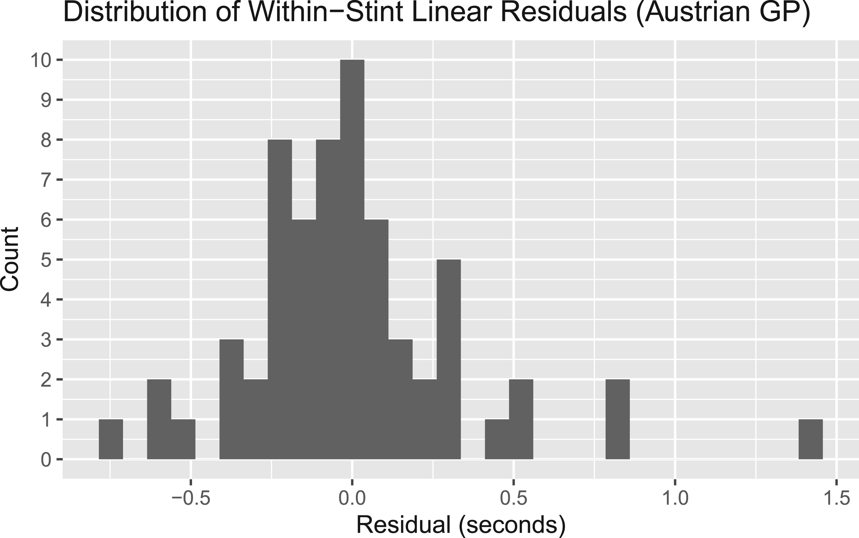
Histogram of residual lap times from within-stint linear trend models for the Austrian Grand Prix. Occasional large positive deviations are visible, motivating the consideration of heavy-tailed observation models.

Fuel mass covariate

Fuel load is included as a lap-level covariate to account for the well-known relationship between vehicle mass and lap time. Because direct fuel mass measurements are not available in the FastF1 API, fuel load is assumed to start at 110 kilograms on lap 1—the regulatory maximum—and decrease linearly to one by the final lap. Although teams may start with slightly less than the maximum, it is operationally reasonable to assume near-zero fuel at race completion due to optimization of starting load.

An alternative assumption would be exponential fuel decay, reflecting the possibility that heavier cars at the beginning of a stint consume fuel at a slightly higher rate. Relative to a linear specification, exponential decay would imply somewhat larger early-stint fuel adjustments and faster convergence later in the stint. In practice, such differences would primarily affect the magnitude of the fuel coefficient $γ$ , while the estimated degradation parameters $α_{t}$ —capturing within-stint performance trends—would change only marginally. Because fuel burn remains smooth across laps and the model is evaluated primarily on predictive performance, modest deviations from linear decay are unlikely to materially affect conclusions.

Code availability

For the interested reader, a Github repository with scripts for pulling data, performing cross validation, and generating the paper itself is available at:

https://github.com/colecappello12/F1_SSM_Paper

Bayesian state-space model

In this section we’ll first briefly review state space models, then describe in detail the process used to model latent degradation rates through the observable lap time process. All models were fitted using the software package Stan (Stan Development Team, 2020).

Background

State-space models (SSMs) are a popular modeling framework for time-series data due to their flexibility. They have found applications in a wide range of areas, from ecological time series (Auger-Méthé et al., 2021), to financial data (Zeng and Wu, 2013), to sports analytics.

State-space models (SSMs) have been widely used in sports analytics to model latent, time-varying performance components and to generate sequential forecasts as new observations become available. For example, Glickman and Stern (2005) develop a state-space framework for modeling evolving team strength in the National Football League, treating underlying ability as a stochastic process inferred from game outcomes. Similarly, Koopman and Lit (2019) propose time-varying strength models for forecasting football match results, while Ötting et al. (2020) apply latent-state models to capture dynamic performance effects in competitive settings. More recently, Michels et al. (2023) and Winkelmann and Michels (2026) employ state-space formulations to model within-match performance dynamics and betting markets, emphasizing interpretable latent processes and probabilistic forecasting. In contrast to much of this literature—where latent states typically represent evolving team or player strength across matches—the present study focuses on intra-race tire degradation in Formula One, where performance evolves within stints and is subject to structural resets induced by pit stops. This domain-specific reset structure, together with fuel effects and degradation dynamics, motivates a tailored state-space specification designed for interpretable and computationally efficient real-time application.

The defining feature of SSMs is their ability to model both a latent unobserved time series via a state equation $α_{t} \sim π (\cdot | α_{t - 1}, y_{1 : t - 1})$ , and an observation time series $Y_{t} | α_{t} \sim f (\cdot | α_{t})$ that consists of measurements which are related to the latent process. SSMs generally make two assumptions:(1) the latent time series evolves as a (typically first order) Markov Process and (2) the observations are independent of one another when we condition on the latent states.

A variety of methods exist for estimation and inference, including the Kalman filter for linear-Gaussian models (Kalman, 1960), Sequential Monte Carlo methods for nonlinear or non-Gaussian systems, and particle MCMC for joint inference on states and parameters (Andrieu et al., 2010). This paper uses Stan and MCMC for model fitting and posterior sampling due to its flexibility and ease of implementation.

Base model specification and parameter interpretation

We start with the observation equation for a driver’s lap times:

y_{t} = α_{t} + γ * f u e l_{t} + ϵ_{t}

(1)

ϵ_{t} \sim N (0, σ_{ϵ}^{2})

(2)

Here $y_{t}$ represents the observed lap time for the driver on lap $t$ . $α_{t}$ represents the true latent pace of the tires after accounting for fuel and degradation. $f u e l_{t}$ is a covariate that represents the derived amount of fuel in kilograms for the driver on lap $t$ , and $γ$ is the estimated increase in lap time due to an additional kg of fuel. Lastly, $ϵ_{t}$ accounts for errors that would result in a lap time being different from $α_{t}$ after accounting for fuel loss. Possible sources of this error include driver mistakes and the presence of other cars.

Now we present the process equation:

α_{t + 1} = (1 - I_{p i t_{t}}) (α_{t} + ν) + I_{p i t_{t}} (α_{r e s e t}) + η_{t}

(3)

η_{t} \sim N (0, σ_{η}^{2})

(4)

where:

\begin{aligned} I_{p i t_{t}} & = {\begin{matrix} 1 & if driver has a new set of tires on lap t+1 \\ 0 & otherwise \end{matrix} \end{aligned}

(5)

t \in {1, 2, \dots, T}

(6)

As mentioned earlier, the latent states $α_{t}$ represent the true pace (or lap time) that the tire is capable of. In the most basic version of the model, we consider a linear rate of decay in lap times, represented by the static parameter $ν$ in the model. However, we allow for error in this decay process by including the term $η_{t}$ . Perhaps most interesting in the process equation is the inclusion of an indicator variable for pit stops. These allow us to reset the degradation process to $α_{reset}$ after the driver puts on a new set of tires, and then continue the degradation process as normal afterwards. Because pit-entry and pit-exit laps are excluded from the analysis, the reset parameter $α_{reset}$ corresponds to the representative post-warmup latent pace on a new set of tires rather than the slower out-lap immediately following a pit stop.

The assumption of linear degradation within a stint serves as a first-order approximation to lap-time evolution over relatively short race segments, which typically span 15–25 laps. In modern race conditions, drivers often target consistent lap times to manage tire wear, resulting in approximately linear trends in observed performance within a stint. While higher-order or nonlinear specifications could be considered, preliminary analysis indicated limited improvement in predictive performance relative to the added complexity. The linear formulation therefore provides an interpretable baseline for modeling degradation dynamics.

Extensions of the basic model

We will propose three extensions to this basic model. The first is to estimate different degradation rates for each tire compound, and the second is to allow the degradation rate $ν$ to increase over time. The final extension will explore the benefits of using a skewed t distribution to model the observation errors.

Extension 1 - compound specific degradation

As mentioned earlier, Formula 1 tires are designed to degrade at different rates by Pirelli (n.d.). Therefore, a natural first extension to make to the base model is to estimate different degradation rates for each compound. With this in mind, our process equation becomes:

α_{t + 1} = (1 - I_{p i t_{t}}) (α_{t} + ν [c o m p o u n d_{t}]) + I_{p i t_{t}} (α_{r e s e t} [c o m p o u n d_{t}]) + η_{t}

(7)

η_{t} \sim N (0, σ_{η}^{2})

(8)

where:

\begin{aligned} c o m p o u n d_{t} & = {\begin{matrix} 1 & if hard tires are used on lap t \\ 2 & if medium tires are used on lap t \\ 3 & if soft tires are used on lap t \end{matrix} \end{aligned}

(9)

As mentioned above, the main thrust of this extension is to estimate different degradation rates and reset points for each tire compound used by the driver.

Extension 2 - time-varying degradation

When tires degrade, there is a loss of mechanical grip as rubber is torn from the surface of the tire. One might well expect that this loss of grip could lead to increased sliding and therefore a compounding of degradation over time. With this in mind, we propose for the second extension a model in which the degradation rate itself increases over time. Under this extension, our process equations become:

\begin{aligned} α_{t + 1} = (1 - I_{p i t_{t}}) (α_{t} + ν_{t}) + I_{p i t_{t}} (α_{r e s e t} [c o m p o u n d_{t}]) + η_{t} \end{aligned}

(10)

ν_{t + 1} = (1 - I_{p i t_{t}}) (ν_{t} + β [c o m p o u n d_{t}]) + I_{p i t_{t}} (v_{r e s e t})

(11)

η_{t} \sim N (0, σ_{η}^{2})

(12)

The most important difference here is that the degradation rate $ν_{t}$ now changes with time. We estimate a parameter $β [c o m p o u n d_{t}]$ for each tire compound that represents an additive increase to the degradation rate that occurs at each time step. It is also important to note that since the degradation rate $ν_{t}$ is allowed to vary with time, we must also include a reset parameter $ν_{r e s e t}$ so that the degradation rate can reset after a pit stop.

Extension 3 - skewed T distribution

Our final extension to the base model is to use a skewed t distribution (Hansen, 1994) for the observation error. Since drivers are given target lap times by their engineers throughout the race, we expect to observe extreme values predominately in the positive direction. For instance, a driver might make a mistake that could lead to an increase of several tenths of a second in lap time, but then return to the target times given by the team. A positively skewed t distribution would capture the possibility of extreme values in the positive direction. The base model would have the same process equation, but the observation equation becomes:

y_{t} = α_{t} + γ * f u e l_{t} + ϵ_{t}

(13)

ϵ_{t} \sim S k e w e d - T (0, σ_{ϵ}^{2}, λ, 2)

(14)

where zero is the mean,

σ_{ϵ}^{2}

is again the variance,

λ

is a skewness parameter that ranges from

- 1

1

, and 2 is the degrees of freedom.

Because of the skewed t distribution’s heavy tails (with lower degrees of freedom), this model should be more robust to outliers than than those using normally distributed errors.

Discussion of priors

In general, we lean on moderately strong priors since we are relatively data poor and have ample information to inform priors. Further, informative priors improve convergence stability and speed, making the model more practical in race conditions.

It should also be noted that lap times often differ by mere tenths of a second. Therefore, priors which at first glance appear very strong, are only moderately so. Given lap times vary by ˜0.5s per stint, priors with SD = 0.1 represent plausible but informative uncertainty levels.

Base model

The priors for our base model are:

σ_{ϵ} \sim N^{+} (.3, {.1}^{2})

(15)

σ_{η} \sim N^{+} (.1, {.1}^{2})

(16)

ν \sim N^{+} (.05, {.1}^{2})

(17)

α_{r e s e t} \sim N (69, {.1}^{2})

(18)

We use a relatively strong prior on the observation standard errors $σ_{ϵ}$ and $σ_{η}$ because the degradation process should have less error than the observation process. The observation process can be affected by driver inconsistencies. Meanwhile the underlying degradation process should remain relatively consistent throughout.

We also use a half-normal prior on the degradation rate to restrict it to be positive, as a negative overall degradation rate would be nonsensical (if the degradation rate is not allowed to change with time as in extension 3). We centered the prior at $.05$ since the scale of the data indicates the degradation rates will be small, but we still believe that the degradation rate should be greater than zero.

Lastly, the prior on the $α_{r e s e t}$ parameters are decided by the long runs done during the free practice sessions. Before the race, Lewis Hamilton’s teammate Charles Leclerc drove a long-run on medium tires suggesting that the race pace of the medium tires would be roughly 69-69.5 seconds per lap. As such, we centered the $α_{r e s e t}$ prior on 69. A similar process was used for the other tracks included in section 5, wherein the reset value was calibrated to the typical lap times done at that track.

Extension 1 - compound specific degradation

The error standard deviation priors for the compound specific degradation model remain the same as before. However, the degradation rate and state resets change since we have to estimate parameters for each tire compound. We have the following extra priors in place of the $ν$ and $α_{r e s e t}$ of before:

α_{r e s e t} [1] \sim N (69.5, {.1}^{2})

(19)

α_{r e s e t} [2] \sim N (69, {.1}^{2})

(20)

α_{r e s e t} [3] \sim N (68.5, {.1}^{2})

(21)

Here $α_{r e s e t} [1]$ is the reset parameter for the hard tire, $α_{r e s e t} [2]$ is the reset parameter for the medium tire, and $α_{r e s e t} [3]$ is the reset parameter for the soft tire. Here, the priors for the resets reflect our prior beliefs that harder tires should start out slower and softer tires will start out faster.

As mentioned in the previous section, there is data from the second free practice session of that race weekend which suggested that the race pace of the medium tires would be 69-69.5 seconds per lap. We use the lower end of this spectrum to account for greater incentive to do faster lap times during the actual race. Then, we make the hard tire reset value a half second slower–and the soft tire a half second faster relative to the medium tires–to reflect our beliefs that the soft tires will start out faster and the hard tires will start out slower.

Extension 2 - time-varying degradation

Here, the error standard deviation priors are the same as the base model, and the reset parameters are the same as for the compound specific degradation model. The main difference is that we include a prior for the degradation state reset $ν_{r e s e t}$ .

ν_{r e s e t} \sim N (0, {.1}^{2})

(22)

Extension 3 - skewed T distribution

For the final extension, we have only updated the observation equation. We let $σ_{ϵ}$ have the same prior as in the base model and put the following prior on the skew parameter $λ$ :

λ \sim N (.5, {.1}^{2})

This prior reflects our belief that the distribution is skewed positively. In fitting the model we used a parameterization of the skewed t distribution in which

λ

–the skewness parameter–can only take on values between

- 1

and

1

. This is reflected in the parameter bounds of the Stan code used to fit the model.

Finally, we do not use a prior on the degrees of freedom because we know that outliers can occur due to driver mistakes or getting stuck behind a slower car, and therefore there is a need for heavy tails. Furthermore, we want the model to fit quickly enough that it can provide strategic information during a race. Adding a prior on the degrees of freedom would make the model take longer to run with little added benefit.

Results

In this section we will discuss the results of fitting the various models. In particular, we will discuss estimates of degradation rates across tire compound and prediction of lap times.

Model selection

Forecasting in this study is performed in a one-step-ahead framework within each race session. For each session, models are estimated using data available up to a given lap and evaluated on subsequent laps using rolling-origin cross-validation. Importantly, race sessions are modeled independently rather than pooled across events, so predictive assessment reflects within-race updating and cross-session robustness rather than multi-race joint training.

We used rolling-origin-recalibration cross validation to perform model selection (Tashman, 2000). We describe the cross validation scheme below. Let $S_{i}$ represent the last lap of stint $i$ , and let $i \in {1, \dots, N}$ where $N$ is the number of stints in the race. Lastly, note that $⌈ x ⌉$ represents the ceiling function for some $x \in R$ . We used the following cross validation scheme:

Stint 1

Fold 1 - Train: $[1, 2, \dots, ⌈ \frac{3}{4} S_{1} ⌉]$ Test: $[⌈ \frac{3}{4} S_{1} ⌉ + 1]$

Fold 2 - Train: $[1, 2, \dots, ⌈ \frac{3}{4} S_{1} ⌉, ⌈ \frac{3}{4} S_{1} ⌉ + 1]$ Test: $[⌈ \frac{3}{4} S_{1} ⌉ + 2]$

…

Fold $\frac{S_{1}}{4}$ - Train: $[1, 2, \dots, S_{1} - 1]$ Test: $[S_{1}]$

…

Stint N

Fold 1 - Train: $[1, 2, \dots, ⌈ \frac{3}{4} S_{N} ⌉]$ Test: $[⌈ \frac{3}{4} S_{N} ⌉ + 1]$

Fold 2 - Train: $[1, 2, \dots, ⌈ \frac{3}{4} S_{N} ⌉, ⌈ \frac{3}{4} S_{N} ⌉ + 1]$ Test: $[⌈ \frac{3}{4} S_{N} ⌉ + 2]$

…

Fold $\frac{S_{N}}{4}$ - Train: $[1, 2, \dots, S_{N} - 1]$ Test: $[S_{N}]$

In this way we perform cross validation on each stint of the driver’s race, and calculate the root mean squared predictive error for each stint so that we can analyze model performance at the stint-level. Letting 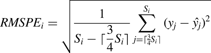${\hat{y}}_{j}$ denote our prediction for the $j t h$ lap, our test statistic is then:

R M S P E_{i} = \sqrt{\frac{1}{S_{i} - ⌈ \frac{3}{4} S_{i} ⌉} \sum_{j = ⌈ \frac{3}{4} S_{i} ⌉}^{S_{i}} (y_{j} - \hat{y_{j}})^{2}}

We performed cross-validation for the base model described above and the three extensions. In addition, we include an AR(1) model with explicit stint resets as a benchmark specification. The AR(1) structure captures short-term autocorrelation in lap times, while the reset mechanism allows the process mean to shift at pit stops in a manner structurally comparable to the proposed state-space model. This specification provides a classical time-series benchmark against which to evaluate the predictive performance of the state-space formulations. Results can be seen in Table 2.

Table 2.

Cross validation results - RMSPE.

	AR(1)	Base Model	Extension 1	Extension 2	Skewed T Dist.
Stint 1	0.457	0.358	0.355	0.386	0.325
Stint 2	0.773	0.673	0.692	0.670	0.601
Stint 3	0.249	0.139	0.140	0.163	0.156
Total	1.478	1.169	1.187	1.218	1.082

Since we obtained samples from the one step ahead predictive distributions using Stan, we also use the Continuous Rank Probability Score (Matheson and Winkler, 1976) with the same cross validation scheme as above to evaluate our probabilistic forecasts. Let $C R P S_{i, j}$ denote the CRPS for the $j t h$ lap in the $i t h$ stint. The overall CRPS for the stint is:

C R P S_{i} = \frac{\sum_{j = ⌈ \frac{3}{4} S_{i} ⌉}^{S_{i}} C R P S_{i, j}}{S_{i} - ⌈ \frac{3}{4} S_{i} ⌉}

In other words, we take the average of each CRPS within a stint to get a stint-level CRPS. Similarly, the overall

\bar{C R P S}

is an average of each stint-level CRPS. The results can be seen in Table 3. Note that a smaller CRPS is indicative of a better forecast.

Table 3.

Continuous rank probability score.

	Base	Extension 1	Extension 2	Skew-T	AR(1)
Stint 1	0.201	0.201	0.220	0.184	0.271
Stint 2	0.377	0.391	0.396	0.316	0.448
Stint 3	0.112	0.115	0.119	0.106	0.148
$\bar{C R P S}$	0.230	0.236	0.245	0.202	0.289

The SSM with skewed t errors is shown to be the best in terms of RMSPE, beating the base model by nearly a tenth. Given the scale of the data, this indicates that the skewed t model performs best on out-of-sample data. Interestingly, this model performs much better than the others in the second stint where there is an extreme outlier in the positive direction. Since performance of the state space models is close among those with normal errors we will still examine them all in the remaining sections, but for out-of-sample prediction we deem the SSM with skewed t errors to perform best.

We see a similar pattern in the Continuous Rank Probability Scores (CRPS) for each of the models (Table 3). The skewed t model beats the other models in all stints, but again performs particularly well in stint 2. The CRPS takes into account the full forecast distribution, so forecasts for the skewed t model are likely able to capture extreme values that the normally distributed models are unable to.

Cross-session predictive validation (2025 Season)

While the Austrian Grand Prix serves as a representative session for model selection and structural comparison, we assess robustness by applying the selected skewed t state-space model and the AR(1) benchmark to 19 race sessions from the 2025 season. Each session is modeled independently using the same rolling-origin cross-validation scheme described in Section 5.1, and race-level predictive metrics are obtained by averaging stint-level scores within each race.

Across the 19 sessions, the state-space model achieves lower RMSPE than the AR(1) benchmark in 15 of 19 races (Table 4). The advantage is slightly more pronounced with CRPS, where the state-space model outperforms the AR(1) specification in 16 sessions. This provides further evidence that the skewed t observation model is more appropriate for uncertainty quantification than Gaussian-based alternatives. On average across races, the skewed t state-space model yields lower predictive error and improved probabilistic calibration, indicating stable performance across heterogeneous circuits and race conditions.

These results suggest that the predictive improvements observed in the Austrian Grand Prix are not isolated to a single session, but reflect a consistent advantage of the state-space formulation relative to a structurally comparable autoregressive benchmark.

Model assessment

For our initial model selection on the Austrian Grand Prix, we obtained posterior samples for the state-space models via Hamiltonian Monte Carlo sampling with 4 chains of 15000 samples each after 15000 burn-in iterations. $\hat{R}$ values for all parameters were less than 1.01, indicating adequate convergence.

For the 19-race cross-validation study, we reduced computation by using two chains with 5,000 post-warmup draws per chain following 5,000 warmup iterations. For certain sessions, additional iterations (15,000–25,000 total) were required to achieve satisfactory $\hat{R}$ and effective sample size. Across sessions, convergence diagnostics were generally acceptable. Divergent transitions were occasionally observed for the skewed t specification, reflecting the increased posterior curvature induced by heavy-tailed likelihoods. Predictive summaries and cross-validation metrics were stable across reruns and were not materially affected by these sampling diagnostics.

It can be seen from Figure 3 that the models all fit the data reasonably well, and are fairly similar. Notably however, the skewed t distribution is not nearly as affected by outliers in the first and second stints, leading to a better fit.

Figure 3.

Fit of the various models with 90% credible intervals. The smoothed predictions are based on the entire time series, as opposed to one-step-ahead predictions which are based solely on observations that occur before the prediction. The smoothed predictions are a basic check that show the model fits the data well. Interestingly, we can see that the skewed t model is not nearly as affected by the outlier on lap 43.

Fitting the first and second extensions of the base model

In the previous section we saw that the skewed t model performed best. While we did expect this model to perform better than the base model, it is surprising that the compound-specific and time-varying degradation models were outperformed by the base model, especially considering that the entire purpose of having different tire compounds in F1 is so that certain compounds will degrade more quickly.

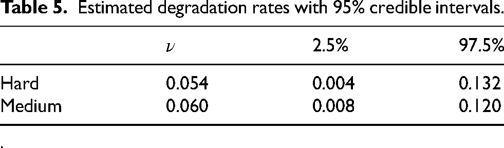
Table 5 shows the estimated values of $ν$ for the first extension to the base model. These estimates are for the hard and medium tires used by Lewis Hamilton in the Austrian Grand Prix, along with bounds for a 95% credible interval. Based on this model, we estimate that Lewis Hamilton loses 5.4 hundredths of a second per lap and 6 hundredths of a second per lap due to tire degradation for hard and medium compound tires respectively, with large uncertainty.

Table 4.

Cross-race CV results. Overall means do not include the Singapore grand prix.

Race	RMSPE (SSM)	RMSPE (AR(1))	CRPS (SSM)	CRPS (AR(1))	Stints
Chinese Grand Prix	0.238	0.240	0.144	0.143	3
Japanese Grand Prix	0.292	0.319	0.165	0.184	2
Bahrain Grand Prix	0.228	0.302	0.145	0.201	3
Saudi Arabian Grand Prix	0.258	0.262	0.162	0.163	2
Emilia Romagna Grand Prix	0.348	0.464	0.206	0.279	3
Monaco Grand Prix	0.661	0.815	0.402	0.481	3
Spanish Grand Prix	0.426	0.637	0.265	0.431	4
Canadian Grand Prix	0.348	0.368	0.216	0.229	3
Austrian Grand Prix	0.360	0.493	0.202	0.289	3
Hungarian Grand Prix	0.550	0.682	0.311	0.389	2
Italian Grand Prix	0.210	0.256	0.128	0.152	2
Azerbaijan Grand Prix	0.527	0.582	0.287	0.346	2
Singapore Grand Prix	0.399	0.352	0.240	0.231	3
United States Grand Prix	1.110	1.063	0.575	0.558	2
Mexico City Grand Prix	0.352	0.342	0.199	0.218	3
São Paulo Grand Prix	0.389	0.387	0.252	0.377	3
Las Vegas Grand Prix	0.368	0.617	0.199	0.392	2
Qatar Grand Prix	0.404	0.564	0.247	0.401	3
Abu Dhabi Grand Prix	0.298	0.351	0.177	0.228	3
Mean Across Races	0.409	0.479	0.238	0.300

Table 5.

Estimated degradation rates with 95% credible intervals.

	$ν$	2.5%	97.5%
Hard	0.054	0.004	0.132
Medium	0.060	0.008	0.120

While we do estimate a slightly higher degradation rate for the medium compound tires, the credible intervals have a large degree of overlap, indicating that the data provides little evidence that there is a difference in degradation rate between the compounds.

From Table 6 it can be seen that the estimated $β$ of the second extension to the base model for the hard tire compound is slightly greater than that for the medium tire compound. Once again however, the credible intervals show a large degree of overlap, indicating little evidence based on the data that the two parameters are different.

Table 6.

Estimated $β$ with 95% credible intervals.

	$β$	2.5%	97.5%
Hard	0.011	0.003	0.020
Medium	0.010	0.002	0.018

Interestingly, the degradation rate $ν$ starts negative, then increases to roughly .175 before a pit stop (see figure 4). This makes sense given that the tires require a warm up period before reaching their optimum operating window(Kelly and Sharp, 2012). Thus, while the skewed t model performed best in terms of predictive accuracy, we can still glean interesting insights from the more complicated models.

Figure 4.

Degradation rates for each lap as estimated by the time-varying degradation model. Interestingly, the degradation rate begins below zero in each stint, indicating the model is capable of capturing a warm-up period for the tires before they begin degrading.

Of course, in both model extensions we see that our degradation estimates do not meaningfully change across the tire compounds used. This is likely why the base model performs better in terms of prediction than our extensions. Another important consideration is that drivers strive to achieve target lap times set by their engineers during a race. Thus, they are not driving at the absolute limit and are actively trying to manage their degradation rates. This partly explains why we tend to see a linear decay. That being said, each stint only has around 20 laps, so we don’t have much data to differentiate what would likely be a small effect size.

Prediction of lap times with uncertainty

One benefit of these models is the ability to quickly assimilate new data points and get predictions for the next lap time with uncertainty intervals. For example, if we run the base model on laps 1-43 to predict lap 44, we get the results seen in Figure 4.

Figures 5 and 6 also support our claim that the models do a good job at forecasting the next lap time. It takes between 15 and 30 seconds to run the base and extension 1 models, giving plenty of time to use the results for decision making in the rest of a lap. In addition, if the fully extended model with increasing degradation rate $ν$ is used, a team could use a certain threshold of $ν$ beyond which they consider a pit stop. In other words, when the degradation rate gets too high, teams can begin seeking an optimal window in which the driver can be pitted. Furthermore, teams could use these results to compare strategies and determine the effects of pitting in optimizing their overall race time Figure 6.

Figure 5.

One-step-ahead prediction of lap 44, given laps 1 to 43. Our point estimate is clearly robust to the outlier on the previous lap. We can also see evidence of the skewed t observation errors in the credible intervals. While the 90% interval appears fairly symmetric, we see that increasing the probability extends the interval farther in the positive direction than in the negative direction (relative to the point estimate).

Figure 6.

One step ahead predictions with 90% credible intervals for the skew t model. Generally speaking, the models do a good job of predicting the next lap time. The uncertainty intervals almost always contain the observation.

Limitations and considerations

Firstly, the Austrian Grand Prix did not have a safety car. Safety cars come onto the track when there has been a serious crash, and all drivers are forced behind the safety car to limit their speeds. As such, driving under safety car conditions drastically reduces degradation since the drivers are limited to much slower speeds. Such a situation could be easily accounted for by extending our model to suspend the degradation process for laps done under safety car conditions.

Secondly, Lewis Hamilton’s drive at the Austrian Grand Prix was fairly uneventful and so he was minimally impeded by the drivers ahead. If a driver gets stuck behind a slower car, this can cause an artificial increase in lap times that isn’t due to tire degradation. The easiest way to address this if necessary is to add a covariate to the observation equation for the distance to the driver ahead. Future work, however, will likely look into more sophisticated ways to address this, such as a multivariate time series with all drivers and dependent errors based on the distance to the driver ahead.

Conclusion

This paper introduced a Bayesian state-space framework for modeling tire degradation in Formula 1 racing, demonstrating that such models can capture the latent deterioration of tire performance while providing interpretable and probabilistic predictions of lap times. Using Lewis Hamilton’s 2025 Austrian Grand Prix as a case study, the proposed approach showed superior predictive performance relative to an AR(1) baseline, particularly when observation errors were modeled with a skewed t distribution to account for asymmetric driver mistakes.

Although degradation rates between tire compounds were not found to differ greatly, teams that have access to more telemetry data could likely discern meaningful differences between tire compounds. The state-space framework’s ability to assimilate new data in real time and output predictive uncertainty makes it a strong candidate for integration into race strategy tools.

Future work should extend the model across multiple drivers to better quantify compound-specific degradation patterns, refine priors using telemetry or surface-temperature data, and explore hierarchical structures for team or track-level effects. Overall, the Bayesian state-space approach provides a statistically principled and computationally efficient foundation for studying tire behavior and optimizing strategy in Formula 1.

Footnotes

ORCID iDs

Cole Cappello

Andrew Hoegh

Funding

The authors received no financial support for the research, authorship, and/or publication of this article.

Declaration of conflicting interests

The authors declared no potential conflicts of interest with respect to the research, authorship, and publication of this article.

References

Ötting

Langrock

Deutscher

, et al. (2020) The hot hand in professional darts. Journal of the Royal Statistical Society: Series A (Statistics in Society) 183(2): 565–80.

Andrieu

Doucet

Holenstein

(2010) Particle markov chain monte carlo methods. Journal of the Royal Statistical Society Series B Statistical Methodology 72(3): 269–342.

Auger-Méthé

Newman

Cole

, et al. (2021) A guide to state–space modeling of ecological time series. Ecological Monographs 91(4): e01470.

Farroni

Sakhnevych

Timpone

(2016) Physical modelling of tire wear for the analysis of the influence of thermal and frictional effects on vehicle performance. Proceedings of the Institution of Mechanical Engineers Part L Journal of Materials Design and Applications 231(1-2): 151–161.

Giles

(2024) Charles leclerc wins italian F1 GP for Ferrari after one-stop gamble. The Guardian, 1 September.

Glickman

Stern

(2005) A State-Space Model for National Football League Scores. In: Anthology of statistics in sports, 23–33. ASA-SIAM Series on Statistics and Applied Mathematics. Philadelphia: Society for Industrial and Applied Mathematics.

Hansen

(1994) Autoregressive conditional density estimation. International Economic Review 35: 705–730.

Kalman

(1960) A new approach to linear filtering and prediction problems. Journal of Engineering for Industry 82(1): 35–45.

Kelly

Sharp

(2012) Time-optimal control of the race car: Influence of a thermodynamic tyre model. Vehicle System Dynamics 50(4): 641–662.

10.

Koopman

Lit

(2019) Forecasting football match results in national league competitions using score-driven time series models. International Journal of Forecasting 35(2): 797–809.

11.

Matheson

Winkler

(1976) Scoring rules for continuous probability distributions. Management Science 22(10): 1087–1096.

12.

Michels

Ötting

Langrock

(2023) Bettors’ reaction to match dynamics: Evidence from in-game betting. European Journal of Operational Research 310(3): 1118–27.

13.

Oehrly

(2025) FastF1: A Python package for accessing and analyzing Formula 1 results, schedules, timing data, and telemetry (version 3.6.0). Available at: https://github.com/theOehrly/Fast-F1 (accessed 6 November 2025).

14.

Pirelli (n.d.) F1 Tires: Details and Technical Data. Available at: https://www.pirelli.com/tires/en-us/motorsport/f1/tires (accessed 6 November 2025).

15.

Tashman

(2000) Out-of-sample tests of forecasting accuracy: An analysis and review. International Journal of Forecasting 16(4): 437–450.

16.

Team Stan Development (2020) Stan: A probabilistic programming language. Journal of Statistical Software 95(1): 1–29.

17.

Todd

Jiang

Russo

, et al. (2025) Explainable Time Series Prediction of Tyre Energy in Formula One Race Strategy. arXiv preprint arXiv:2501.04067.

18.

Winkelmann

Michels

(2026) Momentum effects in team sports: Analyzing the interplay between offense and defense in the NBA, The American Statistician. DOI: 10.1080/00031305.2025.2595980.

19.

Zeng

(2013) State-Space Models: Applications in Economics and Finance. New York: Springer.

A state-space approach to modeling tire degradation in formula 1 racing

Abstract

Keywords

Introduction

Data

Data cleaning

Distributional characteristics

Fuel mass covariate

Code availability

Bayesian state-space model

Background

Base model specification and parameter interpretation

Extensions of the basic model

Extension 1 - compound specific degradation

Extension 2 - time-varying degradation

Extension 3 - skewed T distribution

Discussion of priors

Base model

Extension 1 - compound specific degradation

Extension 2 - time-varying degradation

Extension 3 - skewed T distribution

Results

Model selection

Cross-session predictive validation (2025 Season)

Model assessment

Fitting the first and second extensions of the base model

Prediction of lap times with uncertainty

Limitations and considerations

Conclusion

Footnotes

ORCID iDs

Funding

Declaration of conflicting interests

References