Sage Journals: Discover world-class research

Abstract

Historical data is a valuable asset in sports science, offering insights into athlete development and performance trends. This study explores long-term patterns in competitive swimming by analyzing performance variability over the past 20 years. Instead of clustering similar data points, we grouped entire performance trajectories based on their overall shape, regardless of timing or duration. To model variability, we used a Markov Switching Regression (MSR) model to identify transitions between two volatility regimes: stable (low variance) and unstable (high variance). Only swimmers with at least 50 performances were included to ensure reliable estimates. We then applied the KmlShape clustering algorithm, using Fréchet distance, to group swimmers by the similarity of their volatility profiles and performance patterns. Results showed a link between age, volatility, and competitive outcomes. Swimmers who began earlier tended to have lower volatility and lower performance, while those starting later showed higher volatility and better performance, possibly due to more intense adaptation and pressure in competition. These findings highlight how historical data can inform athlete development. Coaches and analysts can use this approach to understand progression, refine training strategies, and manage performance variability. Future research should expand this framework across sports and demographics for broader applicability.

Keywords

Time series athletic performance volatility markov switching model clustering swimming

Introduction

In recent years, data analysis has become increasingly important in understanding and improving performance across various sports, including swimming. By leveraging advanced analytical techniques, coaches and athletes can gain insights into performance trends and identify areas for enhancement (Costa et al., 2021, Gao, 2006, Mooney et al., 2015, Xie at al., 2017, Woinoski et al., 2020 and Zhang et al., 2020). Longitudinal data, which encompasses repeated measurements of performance variables across multiple time points, allow for a deeper insight into how athletes evolve, adapt, and respond to training regimens, competitions, and recovery periods. These data are valuable not only for optimizing individual performance but also for identifying early indicators of potential injuries, fatigue, or declines in performance (Becerra-Muñoz et al., 2023, Busso et al., 1997, Busso, 2003, Imbach et al., 2022, Marchal et al., 2025 and Philippe et al., 2019).

To model longitudinal data, functional data analysis (FDA) provides a comprehensive framework for analyzing changes in athletic performance. It can be implemented in powerful tools to optimize training programs, improve decision-making processes, and support athletes in achieving peak performance in a sustainable and effective way. When dealing with functional data, FDA models athletes’ performance trajectories, capturing the continuous and uncertain nature of athletic performance, which may vary due to training, competition, and other factors. This approach provides a more nuanced understanding of how performance evolves, including periods of volatility where an athlete’s performance may fluctuate significantly (Forrester and Townend, 2015 Mallor et al., 2010, and Leroy at al., 2018).

One area of particular interest is the analysis of the swimming performance volatility, which refers to the variation in a swimmer’s results over time. To capture this volatility, the Markov Switching Regression model (MSR) is appropriate. Introduced by Goldfeldand and Quandt (1973) and later extended by Hamilton (1989) and Krolzig (1997), MSR has become one of the most popular statistical methods to identify regime shifts in economics and finance (Engel and Hamilton, 1990; Garcia and Perron, 1996; Hamilton, 1988, 1989; Kim and Yoo, 1995 and Kim and Nelson, 1998, among many others). The model is particularly useful when a system exhibits multiple distinct states, such as a swimmer’s performance fluctuating between high and low periods of athletic form. The MSR assumes there are different ”states” of performance (e.g., high, moderate, low) and the transition between these states is probabilistic. These states allow for a better understanding of the unpredictable nature of athletic performance and can assist in developing tailored training strategies. In sports, Sandri et al. (2020) used the Markov switching model to analyze individual basketball shooting performance according to two performance regimes that depend on interactions between players. They considered the effect of a teammate player $i$ on the probability of being in a high-performance regime of a player $j$ . While this applies to team sports, individual sports could also benefit from MSR. The use of MSR with a limited and meaningful number of regimes allows for understanding the stability of an athlete’s performance.

Swimming has been an area of interest for the statistical modeling of performance, where the outcome depends mostly on the swimmer’s own physical and mental abilities and, to a lesser extent, on the opponents (Bouvet et al., 2024; Leroy at al., 2018). Although external elements such as the presence of a coach or competition with other swimmers can play a role in psychological preparation or motivation, they can also introduce variability in a swimmer’s performance. For instance, Wilczyńska at al. (2022) suggest that a positive athlete-coach relationship can significantly impact the psychological state and performance of young athletes. Coaches not only provide technical guidance but also contribute to the mental and emotional readiness of athletes, which is crucial for competitive success. Another study presented by Jane (2015), using a national database of student athletes in Taiwan from 2008 to 2010, suggests that swimmers perform better when competing against faster peers. This indicates that the presence of strong competitors can serve as a motivational factor, pushing swimmers to enhance their performance. These psychological factors, therefore, contribute to the inherent volatility in a swimmer’s performance, as mental resilience and the ability to handle external pressures often determine the consistency of their results.

Swimming performances can vary greatly across different swimmers, age groups, and competition levels. On this basis, clustering methods offer powerful tools for analyzing training data, race results, and physiological measurements. For example, Morais et al. (2022) and Figueiredo et al. (2016) aimed to identify and classify the performance of young swimmers through cluster analysis based on a k-means algorithm. In a more recent study, Bouvet et al. (2024) introduced a novel approach involving double partition clustering of multivariate functional data. The authors used data from inertial measurement units to analyze technical skills, providing insights into biomechanical strategies for front-crawl sprint performance. Additionally, the clustering with Gaussian process models have gained significant attention for evaluating the ranking progression of different performance levels in swimming (Leroy et al., 2023; Veiga et al., 2024). These clustering methods are robust and efficient for many applications. However, studying longitudinal data with different trajectory shapes implies considering the asynchronicity between observations among individuals, the series’ time span, and the overall series shapes.

In this paper, we focus on grouping swimmers according to the similarity of their performance and volatility profiles, allowing for more personalized insights. A promising approach, ”KmlShape,” developed by Genolini et al. (2016), relies on time-series partitioning algorithms based on the shapes of trajectories rather than on classical distances. In this case, the Fréchet distance (Fréchet, 1906) allows for quantifying the similarity between two time series by the minimal distance required to ”transform” one series into another, and hence provides a more accurate comparison of the underlying trends (see, for example, Buchin et al., 2023, Reimering at al., 2018, and Driemel et al., 2015). Adapted to swimming data, KmlShape may capture subtle performance variations and their inherent volatility according to the time-series shape. Consequently, individual data spans, the age at which swimmers start and stop competing, performance trends, and short-term changes are considered for grouping swimmers. By applying such a method, coaches can gain a deeper understanding of how different swimmers’ performances progress over time, identifying distinct profiles within a group of swimmers and facilitating tailored training plans that target specific performance patterns and volatility characteristics.

The purpose of this paper is twofold: (i) to calculate the probabilities of variability in an athlete’s performance, and (ii) to cluster performance and volatility curves. After introducing the methods used to achieve these goals, we will discuss the results in light of the literature and practical considerations for swimming performance stakeholders.

Material & methods

Data description

We consider results from swimming competitions for thousands of athletes spanning from 1976 to 2024, including 163.146 females, 165.332 males, 18 different swimming styles, and publicly available from the French swimming federation (Extranat, 2025) . The dataset consists of multiple irregular, age-based performance time series, with each swimmer having a distinct set of data points at varying time intervals and for different swimming styles, as illustrated in Figure 1. For instance, 32% of female swimmers were tracked for only one year (33% for males), while 6% of females and 5.4% of males were followed for at least five years. The number of participants before 2002 is scarce, with only one swimmer recorded in 1987 and two in 1993. Additionally, the number of observations per swimmer is highly inconsistent. For example, while one swimmer may have only 10 recorded performances, another may have more than 100. To ensure the robustness of the analysis, we limited the dataset to the period from 2002 to 2024. The data were split by sex, and we selected swimmers with more than 50 observations per discipline. Swimmers’ points are calculated using a cubic function, according to WorldAquatics (2025).

Figure 1.

Example of time series for five male swimmers in 100m freestyle competitions.

Formally, let $T$ be the swimming time, and $B$ the base time derived from the current world record (both in seconds). The points $P$ awarded for each competition are calculated as:

P = 1000 {(\frac{B}{T})}^{3} .

Since swimmers start and stop competing at different ages (e.g., starting between 10 and 40 years old, and retiring between 12 and 89 years old), we focused on swimmers who began competing between the ages of 10 and 20, and who retired between the ages of 25 and 40. This sampling strategy helps to avoid bias that could arise from early retirement at younger ages.

To ensure that each athlete’s performance time series was represented over a regular temporal grid—required for Markov Switching Regression (MSR)—we applied cubic spline interpolation. This method constructs a smooth curve that passes through all observed performance values, accommodating the irregular timing of the original measurements. Unlike piecewise linear interpolation, which produces sharp transitions between points, cubic splines yield smooth trajectories with continuous first and second derivatives. This was considered more appropriate for modeling athletic performance, which is expected to evolve gradually over time. We emphasize that this interpolation was used for resampling onto a regular grid, not for noise reduction, and that the interpolated data were subsequently analyzed using a model (MSR) that incorporates temporal dependencies. Spline interpolation was performed using cubic polynomials with knots at the observed data points and no smoothing penalty. (Schumaker, 2007 and Schumaker, 2015).

Markov switching models

Let $s_{t}$ be an unobservable state variable taking values 0 or 1. A standard model for the performance variable $y_{t}$ of an athlete involves two autoregressive models:

y_{t} = {\begin{matrix} α_{0} + β_{s_{t}} y_{t - 1} + ε_{s_{t}}, & s_{t} = 0, \\ α_{0} + α_{1} + β_{s_{t}} y_{t - 1} + ε_{s_{t}}, & s_{t} = 1, \end{matrix}

where

| β_{s_{t}} | < 1

and

ε_{s_{t}}

are i.i.d random variables with mean zero and variance

σ_{s_{t}}^{2}

This setup defines a stationary autoregressive process with mean $α_{0} / (1 - β_{s_{t}})$ when $s_{t} = 0$ , and a different stationary process with mean $(α_{0} + α_{1}) / (1 - β_{s_{t}})$ when $s_{t} = 1$ . If a regime change has occurred in the past, another may occur in the future, which must be considered when forecasting. The model admits two dynamic structures at different levels when $α_{1} \neq 0$ , depending on the state variable $s_{t}$ . In such a case, $y_{t}$ is governed by two distributions with distinct means, and $s_{t}$ determines the switching between these two regimes.

In the MSR framework, the behavior of $y_{t}$ is jointly influenced by the variance $σ_{s_{t}}^{2}$ and the latent state $s_{t}$ . The Markovian nature of $s_{t}$ allows for random and frequent changes in model structure, with the transition probabilities controlling the persistence of each regime. Assuming that $s_{t}$ follows a first-order Markov chain, let $p_{i j}$ for $(i, j) \in {0, 1}^{2}$ denote the transition probabilities, i.e., the probability of being in state $j$ at time $t$ given that the system was in state $i$ at time $t - 1$ . The transition matrix is given by:

\begin{matrix} P & = [\begin{matrix} P (s_{t} = 0 | s_{t - 1} = 0) P (s_{t} = 1 | s_{t - 1} = 0) \\ P (s_{t} = 0 | s_{t - 1} = 1) P (s_{t} = 1 | s_{t - 1} = 1) \end{matrix}] \\ = [\begin{matrix} p_{00} p_{01} \\ p_{10} p_{11} \end{matrix}] . \end{matrix}

The transition probabilities satisfy $p_{i 0} + p_{i 1} = 1$ , for all $i \in {0, 1}$ .

In this model, we estimate the parameters $β_{s_{t}}$ , the transition probabilities $p_{00}$ and $p_{11}$ , the variance $σ_{s_{t}}^{2}$ , and the intercepts $α_{0}$ and $α_{1}$ using maximum likelihood estimation. The statsmodels (2010) library provides a convenient implementation of the MSR model.

In Figure 2, we present the filtered probabilities for the performance regime of an athlete. These refer to estimates of the regime probability at time $t$ , based on all data observed up to and including time $t$ . Regime 0 corresponds to a low-variance, stable performance period, while regime 1 reflects a high-variance, volatile performance period—when the athlete’s performance becomes less predictable. In this study, stability is defined as the percentage of time an individual (or cluster) spends in regime 0, computed as the proportion of observations assigned to the stable regime over the total number of time points.

Figure 2.

(a) Fitted probabilities for regimes 0 and 1 for an athlete in 100m freestyle. The sum of the two probabilities at each time point equals 1. (b) The athlete’s performance with the dominant regime indicated at each time $t$ .

Clustering time series

In this section, we cluster longitudinal performance series with respect to their shapes. Note that series were exploited in their original form, i.e. without time-normalization or resampling. The method is based on an extension of the k-means algorithm, in which we use a ”shape-conservative mean” (Genolini and Falissard, 2010; Hartigan and Wong, 1979; Khan and Ahmad, 2004; Redmond and Heneghan, 2007; Steinley and Brusco, 2007).

The aim of the k-means algorithm is to alternate between two steps. First, the initialization phase defines the mean trajectories of each cluster, calculates the distances between individual trajectories and cluster centroids, and assigns each individual to the nearest cluster. Second, the maximization step estimates the new mean trajectory for each cluster.

For shape-preserving partitioning, we use the clustering algorithm KmlShape (kmlShape library in R), which incorporates several shape-respecting distance metrics. This distance takes a small value when individuals exhibit similarly shaped trajectories, and a large value otherwise. As proposed by Genolini et al. (2016), we use the Fréchet distance to compute the distances between individuals and cluster centers, and the Fréchet mean to construct cluster centroids that reflect the shape-respecting average. The algorithm stops when cluster memberships remain unchanged between iterations $i$ and $i - 1$ . The combination order of individuals is determined in a deterministic manner using an ascending hierarchical classification, where the closest individuals are combined first. This was supported by a visual inspection of clusters afterwards.

We applied this algorithm twice: once to cluster the performance curves of each athlete, and again to cluster the individual stability profiles throughout their swimming careers.

Formally, let $P = {p_{1}, p_{2}, \dots, p_{m}}$ and $Q = {q_{1}, q_{2}, \dots, q_{n}}$ be two time series, such that the discrete Fréchet distance $d_{F}$ between these two sequences is given by:

d_{F} (P, Q) = min_{γ} max_{i} ‖ p_{γ (i)} - q_{i} ‖

where

γ

represents a reparametrization of the curves.

Given a set of trajectories ${T_{1}, T_{2}, \dots, T_{N}}$ , the Fréchet mean is the trajectory $T^{*}$ that iteratively minimizes the sum of squared Fréchet distances:

T * = \arg min_{T} \sum_{i = 1}^{N} d_{F} (T, T_{i})^{2}

The objective function for k-means clustering with Fréchet distance is:

\sum_{k = 1}^{K} \sum_{T_{i} \in C_{k}} d_{F} (T_{i}, μ_{k})^{2}

where

C_{k}

represents cluster

k

and

μ_{k}

denotes the Fréchet mean of that cluster (Genolini et al., 2016).

Statistical analysis

Differences between clusters were evaluated using exploratory one-way Analysis of Variance (ANOVA), followed by post hoc comparisons with Tukey’s p-value adjustment. Marginal mean differences ( $d f$ ) was reported alongside 95% confidence intervals. While these analyses provide descriptive insights into contrasts between clusters, it is important to note that both the ANOVA and post hoc tests were exploratory and not intended for confirmatory inference. Nonetheless, a significance threshold of $p = 0.05$ was applied and consistently reported for interpretive clarity. To assess the contribution of variables related to athlete performance, linear mixed models (LMMs) were fitted. Age (in days), age at the start of competition, and the probability of belonging to the stable regime were standardized and included as fixed effects. Individual participants were modeled as a random effect.

Results

This section presents the results of the analysis conducted on a sample of 282 male swimmers competing in the 100m freestyle event.

Markov switching models

By applying the MSR model to each swimmer’s time series (see Section ”Markov Switching Models”), we estimated the probability at each time point $t$ of being in either regime 0 (stable state), denoted by $P (s_{t} = 0)$ , or regime 1 (unstable state), denoted by $P (s_{t} = 1)$ . These regimes reflect the intra-individual variability in performance, as illustrated in Figure 2. To enable inter-individual comparisons, we focused on the probabilities of belonging to the stable regime (regime 0).

Clustering stability profiles

Clustering the regime 0 probabilities using the KmlShape algorithm with a hierarchical method yielded three distinct groups: 54% of athletes were assigned to Cluster 1 (red), 28% to Cluster 2 (green), and 18% to Cluster 3 (blue), as shown in Figure 3.

An analysis of group-level stability showed that Cluster 1 exhibited 44% stability, while Clusters 2 and 3 demonstrated 46% and 40% stability, respectively. These results indicate that swimmers in Cluster 3 displayed the most volatile performance patterns. The average stability levels significantly differed between clusters ( $d f = 0.036$ , 95% CI 0.021 to 0.051, $p = 0.001$ , $d f = - 0.024$ , 95% CI -0.041 to -0.007, $p = 0.002,$ and $d f = - 0.061$ , 95% CI -0.080 to -0.042, $p = 0.001$ for clusters 1-2, clusters 1-3, and clusters 2-3 comparisons, respectively).

Figure 3.

Transformed (cluster-specific) performance volatility for each cluster generated by the kmlShape algorithm using the discrete Fréchet distance. Each curve represents the aligned shape-based prototype series capturing the characteristic temporal pattern of that cluster. A value below 0.5 indicates a more probable assignment to the stable regime.

We further examined differences in age-related variables across clusters. Specifically, the ages at which athletes began (minimum age) and stopped (maximum age) competing differed significantly between stability groups (see Appendix, Table A1).

Clustering performances curves

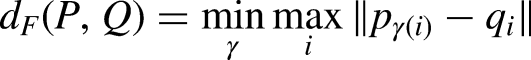
We next applied the same KmlShape algorithm to raw performance trajectories (i.e., points as a function of age in days). This yielded three clusters, illustrated in Figure 4. The first cluster (red, ”low performance”), representing the largest portion of the sample (52% of athletes), had a mean score of 480 points, with interquartile range [420, 548]. The second cluster (green, ”moderate performance”), with a mean of 600 points and interquartile range [547, 652], included athletes with mid-level scores and broader variability. 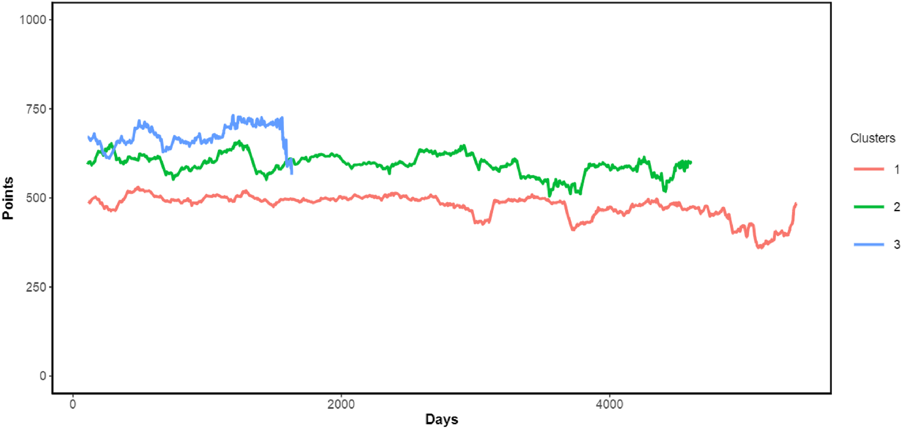The third cluster (blue, ”high performance”) included swimmers with the highest average scores (mean $=$ 680, interquartile range [600, 780]). As illustrated in Figure 5, cluster differences in performance were statistically significant ( $d f = 119$ , 95% CI 115 to 123, $p = 0.001$ , $d f = 194$ , 95% CI 189 to 198, $p = 0.001,$ and $d f = 74.8$ , 95% CI 70.1 to 79.6, $p = 0.001$ for clusters 1-2, clusters 1-3, and clusters 2-3 comparisons, respectively). These findings confirm that the algorithm effectively partitioned athletes based on meaningful differences in performance.

Figure 4.

Transformed (cluster-specific) performance curves for each cluster generated by the kmlShape algorithm using the discrete Fréchet distance.

Figure 5.

Distribution of time series in each performance’s category by stable state (regime 0). The scatter colors represent the probability values of regime 0. (a) Low performance, (b) Moderate performance and (c) High performance

We also compared the age of competition onset and cessation across performance clusters. The mean starting ages were 13, 15, and 16 years for Clusters 1, 2, and 3, respectively (see Appendix, Figure A1). Corresponding stopping ages were 27, 29, and 32 years. These age-related differences were statistically significant (see Appendix, Table A2), underscoring the relevance of age in performance differentiation.

Relationship between stability and performance

Finally, we examined the distribution of athletes within the intersection of these clusters (see Figure 6). We found that 78% of swimmers in the low-performance cluster also belonged to cluster 1 of the stable regime group (regime 0), and 89% of swimmers in the high-performance cluster belonged to cluster 3, the most volatile cluster of the stable regime group. These findings suggest an association between later starting age, greater performance volatility, and higher performance levels. To formally assess this relationship, we fitted a linear mixed model with performance as the dependent variable. Predictors included age (in days), probability of belonging to the stable regime, and competition starting age as fixed effects, and competitors as random effects. All predictors showed significant effects, with the age for a given competition exhibiting the greatest effect over the performance ( $d f = 28$ , 95% CI 27 to 29). Regime probability and competition starting age also contributed in the model ( $d f = 3.38$ , 95% CI 2.38 to 4.39 and $d f = 0.052$ , 95% CI 0.03 to 0.06, respectively. The conditional $R^{2}$ for the model was $67 %$ , indicating substantial explanatory power. Detailed results are provided in Appendix, Table A3.

Figure 6.

Effective of athletes by the stability clustering in each category of performance.

Validation on female sample

To validate our findings, we repeated the full analysis on an independent dataset consisting of 140 female swimmers competing in the 100m freestyle. The results closely mirrored those of the male sample, with three clearly distinguishable clusters for both performance and stability. Age, performance volatility, and competition onset age remained significant predictors. Full results are reported in Appendix, Tables A4-A7 and Figures A2-A3.

Discussion

This study aimed to examine swimmer behavior through two models: the first utilized a Markov Switching Regression (MSR) model to capture performance volatility, assessing fluctuations in individual swimmers’ performance over time. The second model applied a hierarchical clustering algorithm, KmlShape, to group athletes based on the similarity of their performance trajectories, even when these trajectories varied in terms of timing or length, by utilizing the Fréchet distance.

The choice of the number of clusters is critical. In our study, we selected three clusters based on visual inspection of trajectory shapes. We carefully examined the resulting mean trajectories for different values of k (ranging from 2 to 5). The three-cluster solution provided the best compromise between interpretability and distinctiveness. The shapes of the trajectories within each cluster were well-separated, with minimal overlap and high intra-cluster coherence. The hierarchical pre-clustering using the Fréchet distance yielded a clear separation into three main branches. This natural split supported the choice of k = 3 as a meaningful representation of the data’s underlying structure.

It should be noted that clustering was performed on trajectories with their original temporal extents (i.e., not resampled or time-normalized), meaning that differences in duration may have indirectly influenced the Fréchet distance and the resulting cluster structure. In studies where clustering itself is the primary objective, additional preprocessing steps such as time-normalization or resampling would be advisable to minimize the impact of differing temporal extents on the clustering outcome.

After clustering, we may have a key limitation associated with performing statistical tests: when groups are defined using the same data on which the tests are conducted, classical inference procedures such as ANOVA can suffer from inflated Type I error rates due to selection bias. This issue has been formally demonstrated in recent work by Gao et al. (2022), who show that this inflation persists even when clustering and testing are conducted on independent subsets of the data. More recent developments by González-Delgado et al. (2023) offer promising post-clustering inference frameworks that account for the clustering process by conditioning on the selection event, enabling statistically valid p-values and confidence intervals. Although such methods are not yet directly compatible with all forms of clustering—such as those based on trajectory shapes (e.g., KmlShape)—they represent a valuable direction for future research. Incorporating these methods could strengthen the statistical rigor of cluster-based comparisons, especially in applications where cluster separation informs decision-making or hypothesis generation.

Markov Switching models have been widely recognized for their ability to model performance variability in sports, as seen in studies on basketball (Sandri et al., 2020), by positing the existence of multiple regimes or states between which athletes or teams may switch. This approach allows for a nuanced understanding of performance dynamics, accounting for significant variations due to factors like physical condition, mental state, or external circumstances. Our findings align with the broader literature, highlighting the importance of regime-switching in capturing performance volatility.

However, the specification of the number of regimes and the structure of transition probabilities remain a critical aspect of MSR model application. Incorrect choices in this regard can significantly influence the model’s performance and lead to misleading or unstable results (Song and Woźniak, 2020). In our analysis, testing with more than two regimes resulted in inconsistent and sometimes implausible probability estimates, such as constant probabilities of zero, suggesting that a higher number of regimes introduced instability in probability distributions rather than improving the model in capturing performance dynamics. This underlines the importance of considering the number of regimes carefully in relation to the specific aims of the study. For our purpose of examining volatility, a two-regime model —representing stable (i.e. low variance) and unstable (i.e. high variance) performance states– proved to be sufficient.

Additionally, the robustness of the MSR model relies on having a sufficient number of observations. Therefore, we restricted our analysis to swimmers with at least 50 data points to ensure the reliability of the model and the robustness of our findings.

After estimating the probability of being in the stable regime (regime 0) for each swimmer, we proceeded to group athletes based on their volatility profiles using the KmlShape clustering algorithm. Using a hierarchical approach paired with the Fréchet distance, it resulted in three distinct clusters based on performance volatility, which were associated with the athletes’ competition start and end ages. Clusters 1 and 2 represented athletes with relatively stable performance, with athletes in these groups beginning their careers at ages younger than 14. This period of early development is characterized by significant physical and psychological changes that can lead to fluctuations in performance. As swimmers grow and adapt to new training regimes, these fluctuations may occur as they develop new skills, adjust to physical changes, and encounter the pressures of competitive environments (Bergeron et al., 2015; Malina, 2011). In contrast, Cluster 3 represented athletes with higher volatility, typically associated with later onset and more significant fluctuations as athletes adapt to the physical demands of the sport.

When we applied the same clustering approach to performance points (as a function of age), we identified three clusters, each corresponding to distinct performance levels. The majority of athletes fell into the first cluster, indicating lower performance levels. Notably, the average age at which athletes in this cluster began competing was below 13, coinciding with the period of puberty and the adolescent growth spurt (Malina, 2011). During this time, athletes are undergoing significant physical changes, which may initially hinder their performance. However, as athletes mature physically and mentally, their performance typically improves with the right training regimen.

While young male and female athletes exhibit similar performance levels before puberty, clear differences emerge during and after puberty. These differences are primarily attributed to hormonal changes, relative ages (Difernand et al., 2025), and the resulting physical developments (Handelsman, 2017; Handelsman et al., 2018). The impact of these physiological changes on athletic performance underscores the importance of considering gender-specific developmental trajectories in training and performance analysis.

Our analysis revealed several interesting trends. Younger athletes tended to exhibit more stable performance but also performed at lower levels compared to older athletes. Early starters often remain in the developmental phase of their careers, leading to greater consistency but lower overall performance. In contrast, athletes who start later may experience greater physiological changes as they adapt to the demands of swimming, resulting in more volatile performance patterns. This is further illustrated by the data in Figure 5 and Appendix, Table 2.

The adaptation process of late-starting athletes, coupled with the intense pressure of competing against more experienced peers, can contribute to psychological stress. This stress, in turn, can lead to performance volatility, as athletes struggle to maintain focus and composure during competitions (Özdemir, 2019). These findings highlight the complex interplay between physical development, training, and psychological factors in determining athlete performance.

To generalize the findings of this study, future research should consider expanding the scope to include other sports disciplines and to incorporate both male and female athletes in the sample. Access to a larger, more diverse dataset could provide valuable insights into the factors driving the observed trends, including the role of training methods, physiological factors, or external influences such as coaching style and peer dynamics. Exploring these aspects could provide a more comprehensive understanding of the determinants of performance volatility and strategies for improving athletic outcomes. In addition, incorporating more data into the analysis enhances the potential for predictive modeling (Saavedra et al., 2010; Silva et al., 2007). By training models on broader and more varied performance histories, we can better anticipate future outcomes, identify early signs of performance shifts, and support data-driven decision-making in training and competition planning using functional data.

Conclusion

This study offers key insights into swimmer performance volatility and stability. Our results suggest that younger swimmers tend to exhibit lower volatility but also lower performance, with age playing a critical role in both the stability of performance and the development of competitive abilities. These findings underscore the importance of considering age-related factors when evaluating athlete performance.

From a practical standpoint, these results emphasize the value of historical performance data for coaches. By understanding not only an athlete’s performance but also their volatility, coaches can better tailor training programs to meet individual needs, thereby improving performance and reducing volatility. This approach could significantly enhance the efficiency of training regimens and support athletes in reaching their full potential.

Supplemental Material

sj-pdf-1-san-10.1177_22150218261419295 - Supplemental material for Analyzing swimming performances based on series dynamics and volatility

Supplemental material, sj-pdf-1-san-10.1177_22150218261419295 for Analyzing swimming performances based on series dynamics and volatility by Chayma Daayeb, Arij Amiri, Robin Pla and Frank Imbach in Journal of Sports Analytics

Footnotes

ORCID iD

Frank Imbach

Author contributions

Conceptualisation, C.D., F.I.; methodology and investigation, C.D., A.A., F.I.; data curation, R.P., F.I.;recruitment, R.P.; resource development, C.D., F.I.; formal analysis, C.D., A.A., F.I.; writing original draft preparation, C.D., F.I.; writing-review and editing, C.D., F.I.; supervision, F.I.; project administration, F.I. All authors have read and agreed to the published version of the manuscript.

Funding

The author(s) received no financial support for the research, authorship, and/or publication of this article.

Declaration of conflicting interests

The authors declared no potential conflicts of interest with respect to the research, authorship, and publication of this article.

Data availability statement

Correspondence and requests for materials should be addressed to F.I.

Supplemental Material

Supplemental material for this article is available online.

References

Becerra-Muñoz

Wang

Pérez-Tejero

(2023) Women’s wheelchair basketball lineup analysis at the Tokyo 2020 paralympic games: Game related statistics explaining team sport performance. Frontiers in Sports and Active Living 5: 1281865. doi: 10.3389/fspor.2023.1281865.

Bergeron

Mountjoy

Armstrong

, et al. (2015) International Olympic committee consensus statement on youth athletic development. British Journal of Sports Medicine 49(13): 843–851.

Bouvet

Kolei

Marbac

(2024) Investigating swimming technical skills by a double partition clustering of multivariate functional data allowing for dimension selection. The Annals of Applied Statistics 18(2): 1750–1772.

Buchin

Driemel

Rohde

(2023) Approximating (k,l)-median clustering for polygonal curves. ACM Transactions on Algorithms 19(1): 1–32.

Busso

(2003) Variable dose-response relationship between exercise training and performance. Medicine and Science in Sports and Exercise 35(7): 1188–1195.

Busso

Denis

Bonnefoy

, et al. (1997) Modeling of adaptations to physical training by using a recursive least squares algorithm. Journal of Applied Physiology 82(5): 1685–1693.

Costa

Silva

Santos

, et al. (2021) Framework for intelligent swimming analytics with wearable sensors for stroke classification. Sensors (Basel) 21(15): 5162.

Difernand

Mallet

De Larochelambert

, et al. (2025) A survival analysis of dropout among French swimmers. Frontiers in Sports and Active Living 7: 1509306.

Driemel

Krivošija

Sohler

(2015) Clustering time series under the fréchet distance. In: Proceedings of the 2016 Annual ACM-SIAM Symposium on Discrete Algorithms (SODA), pp.766–785.

10.

Engel

Hamilton

(1990) Long swings in the dollar: Are they in the data and do markets know it?. American Economic Review 80: 689713.

11.

Federation Française de natation (2025) Extranat. Available at: https://ffn.extranat.fr/ (accessed April 18, 2025).

12.

Figueiredo

Silva

Sampaio

, et al. (2016) Front crawl sprint performance: A clusterAnalysis of biomechanics, energetics,Coordinative, and anthropometric determinants in young swimmers. Human Kinetics, Motor Control 2016 20: 209–221.

13.

Forrester

Townend

(2015) The effect of running velocity on footstrike angle—A curve-clustering approach. Gait & posture 41: 26–32.

14.

Fréchet

(1906) Sur Quelques Points Du Calcul Fonctionnel. Paris: Rendiconti del Circolo Matematico di Palermo (1884-1940).

15.

Gao

Bien

Witten

(2022) Selective inference for hierarchical clustering. arXiv, Statistics, Methodology, 2012.02936.

16.

Gao

(2006) Sports video analysis. In: Proceedings of the 12th international multi-media modelling conference, Beijing, China.

17.

Garcia

Perron

(1996) An analysis of the real interest rate under regime shifts. Review of Economics and Statistics 78: 111–125.

18.

Genolini

Falissard

(2010) kml: K-means for longitudinal data. Computational Statistics 25(2): 317–328.

19.

Genolini

Ecochard

Benghezal

, et al. (2016) kmlShape: An efficient method to cluster longitudinal data (time-series) according to their shapes. PloS one 11(6): e015073.

20.

Goldfeld

Quandt

(1973) A markov model for switching regressions. Journal of Econometrics 1(1): 3–15.

21.

González-Delgado

Cortés

Neuvial

(2023) Post-clustering Inference under Dependency. arXiv, Statistics, Methodology, 2310.11822.

22.

Hamilton

(1988) Rational-expectations econometric analysis of changes in regimes: An investigation of the term structure of interest rates. Journal of Economic Dynamics and Control 12: 385–423.

23.

Hamilton

(1989) A new approach to the economic analysis of nonstationary time series and the business cycle. Econometrica: Journal of the Econometric Society 57(2): 357–385.

24.

Handelsman

(2017) Sex differences in athletic performance emerge coinciding with the onset of male puberty. Clinical Endocrinology (Oxf) 87(1): 68–72.

25.

Handelsman

Hirschberg

Bermon

(2018) Circulating testosterone as the hormonal basis of sex differences in athletic performance. Endocrinology Reviews 39(5): 803–829.

26.

Hartigan

Wong

(1979) algorithm AS 136:A K-means clustering Algorithm. Journal of the Royal Statistical Society Series C (Applied Statistics) 28(1): 100–108.

27.

Imbach

Sutton-Charani

Montmain

, et al. (2022) The use of fitness-fatigue models for sport performance modelling: Conceptual issues and contributions from machine-learning. Sports Medicine Open 8(1): 1–6.

28.

Jane

W-J

(2015) Peer effects and individual performance: Evidence from swimming competitions. Journal of Sports Economics 16(5): 531–539.

29.

Khan

Ahmad

(2004) Cluster center initialization algorithm for k-means clustering. Pattern Recognition Letters 25(11): 1293–1302.

30.

Kim

Nelson

(1998) Business cycle turning points, a new coincident index, and tests of duration dependence based on a dynamic factor model with regime switching. Review of Economics and Statistics 80: 188–201.

31.

Kim

Yoo

(1995) New index of coincident indicators: A multivariate markov switching factor model approach. Journal of Monetary Economics 36: 607–630.

32.

Krolzig

(1997) Markov-switching Vector Autoregressions: Modelling, Statistical Inference, and Application to Business Cycle Analysis. New York: Springer.

33.

Leroy

Latouche

Guedj

, et al. (2023) Cluster-specific predictions with multi-task Gaussian processes. Journal of Machine Learning Research 24(5): 1–49.

34.

Leroy

Marc

Dupas

, et al. (2018) Functional data analysis in sport science: Example of swimmers’ progression curves clustering. Applied Sciences 8(10): 1766.

35.

Malina

(2011) Skeletal age and age verification in youth sport. Sports Medicine 41(11): 925–47.

36.

Mallor

Leon

Gaston

, et al. (2010) Changes in power curve shapes as an indicator of fatigue during dynamic contractions. Journal of Biomechanics 43: 1627–1631.

37.

Marchal

Benazieb

Weldegebriel

, et al. (2025) Statistical flaws of the fitness fatigue sports performance prediction model. Scientific Reports 15: 3706.

38.

Mooney

Corley

Godfrey

, et al. (2015) Analysis of swimming performance: Perceptions and practices of US-based swimming coaches. Journal of Sports Sciences 34: 997–1005.

39.

Morais

Barbosa

Neiva

, et al. (2022) Young swimmers’ classification based on performance and biomechanical determinants: Determining similarities through cluster analysis. Motor control 26(3): 396–411.

40.

Özdemir

(2019) The investigation of elite athletes’ psychological resilience. Journal of Education and Training Studies 7(10): 47–57.

41.

Philippe

Borrani

Sanchez

, et al. (2019) Modelling performance and skeletal muscle adaptations with exponential growth functions during resistance training. Journal of Sports Sciences 37(3): 254–261.

42.

Redmond

Heneghan

(2007) A method for initialising the k-means clustering algorithm using kd-trees. Pattern Recognition Letters 28(8): 965–973.

43.

Reimering

Muñoz

McHardy

(2018) A fréchet tree distance measure to compare phylogeographic spread paths across trees. Scientific Reports 8: 17000.

44.

Saavedra

Escalante

Rodriguez

(2010) A multivariate analysis of performance in young swimmers. Pediatric exercise science 22(1): 135–151.

45.

Sandri

Zuccolotto

Manisera

(2020) Markov switching modelling of shooting performance variability and teammate interactions in basketball. Journal of the Royal Statistical Society Series C: Applied Statistics 69(5): 1337–1356.

46.

Schumaker

(2007) Spline Functions: Basic Theory. 3rd ed. Cambridge: Cambridge University Press.

47.

Schumaker

(2015) Spline Functions: Computational Methods. Society for Industrial and Applied Mathematics.

48.

Seabold

(2010) statsmodels: Econometric and statistical modeling with python. 9th Python in Science Conference.

49.

Silva

Costa

Oliveira

, et al. (2007) The use of neural network technology to model swimming performance. Journal of sports science & medicine 6(1): 117.

50.

Song

Woźniak

(2020) Markov Switching. Oxford: Oxford Research Encyclopedia of Economics and Finance.

51.

Steinley

Brusco

(2007) Initializing k-means batch clustering: A critical evaluation of several tech niques. Journal of Classification 24(1): 99–121.

52.

Veiga

Grenouillat

Rodríguez-Adalia

, et al. (2024) Ten-year evolution of world swimming trends for different performance clusters: A Gaussian model. International Journal of Sports Physiology and Performance 19(12): 1391–1399.

53.

Wilczyńska

Walczak-Kozłowska

Alarcón

, et al. (2022) Dimensions of athlete-coach relationship and sport anxiety as predictors of the changes in psychomotor and motivational welfare of child athletes after the implementation of the psychological workshops for coaches. International Journal of Environmental Research and Public Health 19(6): 3462.

54.

Woinoski

Harell

Bajic

(2020) Towards Automated Swimming Analytics Using Deep Neural Networks. arXiv.

55.

World Aquatics (2025) Available at: https://www.worldaquatics.com/swimming/points (accessed April 18, 2025).

56.

Xie

Nie

, et al. (2017) Machine learning of swimming data via wisdom of crowd and regression analysis. Mathematical Biosciences and Engineering 14: 511–527.

57.

Zhang

Chen

Chan

, et al. (2020) Intelligent sports performance scoring and analysis system based on deep learning network. In: Proceedings of the 3rd international conference on artificial intelligence and big data (ICAIBD), Chengdu, China.

Supplementary Material

Please find the following supplemental material available below.

For Open Access articles published under a Creative Commons License, all supplemental material carries the same license as the article it is associated with.

For non-Open Access articles published, all supplemental material carries a non-exclusive license, and permission requests for re-use of supplemental material or any part of supplemental material shall be sent directly to the copyright owner as specified in the copyright notice associated with the article.

0.00 MB

0.22 MB