Sage Journals: Discover world-class research

Abstract

This study examines whether a simple model based on expected goals (xG) can generate accurate forecasts and identify profitable signals in football betting markets. The model uses recent xG to estimate win–draw–loss probabilities via a Skellam distribution, with isotonic regression applied for calibration, and evaluates the performance over eleven Bundesliga seasons (2014/15 through 2024/25). While bookmaker odds tend to exhibit superior statistical calibration, the xG-based model captures certain signals not fully reflected in market prices. In simulated betting, the model yields a return on investment of approximately 10% using average market odds, increasing to nearly 15% under the best available prices. Profits stem predominantly from home win bets, while backing away wins is consistently loss-making. The results show some robustness to modelling choices, though profitability varies considerably by season and bet type. The study highlights the potential of simple models as practical tools for identifying predictive value in structured football data.

Keywords

football forecasting expected goals (xG)betting markets value betting Bundesliga

Introduction

Forecasting football match outcomes has drawn sustained academic and practitioner interest, particularly as granular performance metrics such as expected goals (xG) have enabled more systematic modelling of team strength and match dynamics. Initially developed within online analytics communities, xG is now deeply embedded in modern football practice. English Premier League clubs, for instance, use xG-based frameworks to inform player recruitment and tactical decisions, supported by evidence of substantial value generation through data-informed strategies (Tippett, 2019, 2024). These models evaluate shot quality and efficiency rather than raw outcomes such as scored goals, allowing probabilistic assessments that are more robust to randomness and variance in match results. They also provide an empirical basis for estimating outcome probabilities that can be compared and potentially combined with those implied by bookmaker odds. Methodologies used to evaluate football markets mirror techniques in financial and economic forecasting, where market data act as proxies for latent probabilities (Kain and Logan, 2014). Even when their forecasts are not perfectly calibrated, such models may capture distinct patterns or structural tendencies that are underweighted or overlooked by the market.

Despite their appeal, predictive models in football face the sport’s inherent complexity. Outcomes are shaped by low-frequency, high-impact events and influenced by a wide range of factors. Betting markets, while often information-efficient, embed structural features and behavioural biases that complicate the interpretation of odds. These challenges necessitate models that are both statistically coherent and robust to real-world constraints.

This paper contributes to the literature by systematically evaluating the predictive and economic value of a simple, robust model for the German Bundesliga. Using eleven seasons of data, it applies this xG-based framework to convert recent match performance into outcome probabilities, finetuned through isotonic regression. These forecasts are compared with bookmaker-implied probabilities in terms of calibration and predictive accuracy and used to identify value bets in simulated betting strategies. A dedicated robustness check also examines how much of the economic performance is attributable to the isotonic calibration layer. While xG-based forecasts are slightly less well calibrated than market odds, they capture certain signals that translate into consistent, albeit modest, profitability: average market odds yield a return on investment (ROI) of about 10%, increasing to nearly 15% under best-available prices. Selective strategies optimised for ROI or Sharpe ratio can exceed 10%, though based on a relatively small number of bets. Notably, home win bets generate the bulk of profits, while away bets remain persistently unprofitable. These findings remain largely robust across seasons, parameter variations and staking approaches.

Conceptually, this study is related to the xG-based performance framework of Brechot and Flepp (2020), who analyse how random variation in finishing and goalkeeping distorts observed results and construct xG-based efficiency ratios and league tables for ex-post assessment of team performance. In contrast, the present paper examines whether a similarly parsimonious xG-driven model can deliver economically valuable ex-ante forecasts and reveal mispricings in football betting markets.

The paper is organised as follows. In Section “Previous research”, a structured overview of prior research on football forecasting is provided, covering statistical models, market-based approaches, hybrid methods and supporting literature. In Section “Data and modelling framework”, the data are introduced and the modelling framework is outlined, based on expected goals and the derivation of probabilistic forecasts. Furthermore, a post-calibration finetuning of the model forecasts through isotonic regression is discussed. Potential value betting strategies are described in Section “Devising a betting strategy”. Besides the identification of opportunities and baseline benchmarks, several money management strategies are introduced. Section “Results” presents the main results, beginning with an evaluation of the model’s calibration and predictive accuracy and then evaluating the profitability of betting strategies after threshold optimisation, including performance by bet type. In Section “Robustness and sensitivity analysis”, the robustness and sensitivity of results to key modelling choices are explored, focusing on elements such as the historical xG calibration window, odds selection, staking method and the use or omission of isotonic calibration. Section “Conclusion and outlook” concludes and outlines avenues for future research.

Previous research

Football outcome prediction has been studied through three principal lenses: statistical modelling, market-based inference and hybrid or machine learning approaches. Each reflects a different philosophy of how match dynamics and uncertainty can be understood, with implications for model calibration, practical implementation and relevance to betting contexts.

Statistical modelling approaches

Statistical models have long underpinned football forecasting, with Poisson-based methods providing the foundation. Maher (1982) modelled goals as independent Poisson processes linked to team strengths; Dixon and Coles (1997) introduced temporal weighting and corrections for low-scoring outcomes and inefficiencies.

The Skellam distribution, capturing the difference between two Poisson variables, naturally models win-draw-loss results. Karlis and Ntzoufras (2009) used Bayesian estimation in this setting, while Xenopoulos (2016) confirmed its empirical validity. However, the assumption of goal independence is often disputed. Bivariate Poisson models address this by introducing scoring correlation, improving the modelling of draws, as shown by Karlis and Ntzoufras (2003) and Groll et al. (2018). More flexible dynamic or latent-state approaches – e.g. the score-driven multivariate models of Koopman and Lit (2015) and the copula-structured hidden Markov model of Ötting et al. (2023) – enhance fit but reduce interpretability and increase calibration effort. Michels et al. (2025) cater for a more general dependence structure and show that richer correlation patterns can substantially improve fit.

Recent xG models estimate scoring potential from shot-level data – e.g. location, angle, assist type – offering more stable proxies for team strength than realised goals. Brechot and Flepp (2020) use such an xG framework to disentangle luck from skill in realised results, constructing xG-based league tables and offensive/defensive efficiency ratios that show how short runs of matches can diverge from underlying performance. Fu (2024) and Mead et al. (2023) highlight how feature choice and data source impact predictive accuracy. Dynamic rating systems such as Elo and pi-ratings, which update based on results, goal margins and opponent strength, remain widely used and have outperformed official rankings in predictive tasks (Hvattum and Arntzen, 2010; Lasek et al., 2013). A recent comprehensive treatment of these models and their implementation in football contexts is provided by Egidi et al. (2025).

Together, these statistical approaches form the backbone of football forecasting, with ongoing work focused on refining match dynamics, enriching input features and improving evaluation.

Market-based models and efficiency

Betting markets serve as a benchmark for probabilistic forecasts, aggregating public sentiment, expert judgement and contextual factors. While generally effective at incorporating information, they show structural and behavioural patterns that can lead to persistent mispricing – creating scope for model-based strategies.

A key research strand evaluates market efficiency ex post. Forrest et al. (2005), Goddard and Asimakopoulos (2004) and Vlastakis et al. (2009) show that while bookmaker odds are well calibrated, they are not fully efficient. Mispricings stem from overrounds, limited competition, pricing conventions and behavioural biases. Using a combination of Monte Carlo simulations and multi-season European football odds, Winkelmann et al. (2024) caution that many reported anomalies are consistent with sampling variation and find little evidence of persistent, exploitable inefficiencies. Work on value betting explores profitability. Franck et al. (2010) find better pricing accuracy on exchanges than with bookmakers. Feng et al. (2016) infer scoring intensities from odds using a Skellam framework and improve calibration by adjusting for draw overpricing. Kaunitz et al. (2017) use simple filters to identify profitable strategies, while Constantinou et al. (2013) apply Bayesian networks that outperform odds. Egidi et al. (2025: Chapter 7) provide a recent, systematic comparison between state-of-the-art statistical models and bookmaker odds, likewise concluding that margins and small, unstable mispricings leave limited scope for persistent outperformance.

Implied probability calibration is central. Strumbelj (2014) proposes margin-adjusted methods to reconstruct fair odds and enable comparison with model forecasts. Behavioural biases are well documented. Franke (2020) and Brown and Yang (2021) examine phenomena such as the favourite-longshot bias and other pricing distortions. Drawing on in-play Bundesliga odds and volumes, Ötting et al. (2025) find that bettors behave as if equalisers create strong momentum, even though estimated win probabilities change little, underscoring the psychological component of pricing. Brown and Yang (2019) show that forecast accuracy improves with crowd diversity and market depth.

In-play and high-frequency studies offer a dynamic view. Croxson and Reade (2014) show that exchange odds adjust almost instantaneously to goals and display little subsequent drift, while Winkelmann and Deutscher (2025) find no systematic adjustment of odds or stakes in the seconds leading up to goals in the Bundesliga, suggesting that markets neither strongly anticipate nor underreact to such events. Michels et al. (2023) and Ötting et al. (2024) document strong shifts in trading volume and stake distribution around short-term performance swings, revealing limits to real-time efficiency.

Overall, markets appear broadly – but not fully – efficient. Odds embed rich information but remain subject to frictions and behavioural distortions.

Hybrid and machine learning approaches

Machine learning (ML) has become prominent in football prediction, offering tools to model nonlinear patterns and feature interactions. These approaches often extend classical models, especially when leveraging domain-specific inputs like expected goals, team ratings or recent form. Methods include tree-based ensembles, support vector machines (SVM), neural networks and probabilistic graphical models.

Bayesian networks capture uncertainty and structural dependencies in outcomes. Joseph et al. (2006) demonstrated early promise, with later work integrating form and rating dynamics. Comparative studies benchmark ML models against Poisson or Elo-type baselines. Singh et al. (2025) and Fischer and Heuer (2025) evaluate families like SVMs, random forests and neural networks, often concluding that feature quality matters more than model class.

Some work assesses profitability as well as accuracy. Stübinger and Knoll (2018) and Hubacek et al. (2019) simulate betting strategies using ML forecasts, highlighting the importance of calibrated inputs and market-derived features. Tree-based methods generally perform well, but rely heavily on effective feature engineering. Baboota and Kaur (2019), Kozak and Glowania (2021) and Edalatpanah and Hess (2024) report strong results across top European leagues, particularly for high-confidence predictions. Berrar et al. (2024) likewise emphasise that thoughtful feature design often outweighs algorithmic complexity.

Recent work integrates spatiotemporal and player-level data. Hewitt and Karakus (2023) enhance xG models with player roles and context, while Bialkowski et al. (2014) use unsupervised learning to extract team formations – signalling a shift toward tactical modelling beyond team aggregates. Explainability is gaining focus. Cavus and Biecek (2022) apply SHAP and LIME to xG-based models, improving interpretability and supporting transparent decision-making.

Together, machine learning methods offer promising applications to football forecasting, though their success depends critically on feature design, calibration and interpretability.

Other approaches and supporting literature

Beyond core modelling, related work addresses evaluation metrics, betting strategy, behavioural factors and data resources – all shaping how football forecasting systems are developed and applied.

A key focus is betting strategy and bankroll management. The Kelly criterion (Kelly, 1956) remains foundational for sizing bets under uncertainty. Uhrin et al. (2021) show that fractional Kelly offers favourable risk-adjusted returns with noisy models. Buchdahl (2003) provides a widely cited guide on fixed-odds betting, covering expected value and margin correction. Kopriva (2015) contrasts utility theory with observed behaviour, revealing consistent deviations from optimal staking. Effective capital allocation is thus as important as accurate prediction.

On model evaluation, Wunderlich and Memmert (2020) provide a taxonomy of forecasting approaches, from expert-driven to ML hybrids. Wheatcroft (2022) recommends log-loss and Brier scores over ranked probability scores in football, stressing calibration and sharpness. Behavioural and heuristic forecasting is another active strand. Tippett (2017) argues that simple, data-driven methods can rival expert judgement. His later works (Tippett, 2019, 2024) further support the consistency of analytical approaches over intuition, echoing broader behavioural economics insights.

Finally, new data resources enhance transparency and reproducibility. Dubitzky et al. (2019) introduce an open-access database spanning over 200,000 matches across 52 leagues. Bassek et al. (2025) expand this with Bundesliga-specific spatiotemporal data, enabling more granular tactical analysis.

Against a backdrop of increasingly complex forecasting methods, this study examines whether a straightforward, interpretable model can nevertheless uncover reliable signals that reflect structural inefficiencies and offer predictive leverage over market odds.

Data and modelling framework

Data

The setup uses match data and xG values for the 1. Bundesliga during the eleven seasons from 2014/15 to 2024/25 (source: https://understat.com). This is complemented by bookmaker and betting exchange data for the same period (source: https://www.football-data.co.uk). The latter consists of closing odds, i.e. the last odds before a match starts. For each time point, the average quotes are obtained – with the panel typically consisting of about 15 providers each. This ensures a sufficiently representative picture of market-implied probabilities as well as liquidity for any bets to be placed at these odds. Section “Robustness and sensitivity analysis” examines how the results change when the ‘best’ available odds are used instead of the averages.

Table 1 provides a descriptive overview of the overall dataset. With 18 teams in the league, there are 306 matches per season, yielding a total of 3,366 over the course of the analysis. On average, teams score between one and two goals per match, with considerable variation. Up to eight goals per team are observed in individual matches. The expected goals largely mimic this picture, although with less variation and extremes (an xG value of 0.0 indicates that a team has not attempted a single shot in the entire match). Across all matches, the average expected goals for home teams (1.66) exceeds that of away teams (1.32), indicating a typical home advantage of approximately 0.34 xG. This asymmetry is reflected in both actual and expected goal statistics and is implicitly captured in the model through venue-specific xG aggregation (see Section “Generating predictions from historical xG”).

Table 1.

Statistics for goals, xG, match outcomes and odds.

Number of matches	3,366
A. Goal statistics
	Home team		Away team
Mean	1.69		1.34
Median	1		1
Standard deviation	1.39		1.23
Minimum	0		0
Maximum	8		7
B. Expected goals (xG)
	Home team		Away team
Mean	1.66		1.32
Median	1.50		1.16
Standard deviation	0.97		0.84
Minimum	0.00		0.00
Maximum	6.88		6.50
C. Match outcome distribution
	Home win	Draw	Away win
Statistic	44.5%	24.9%	30.5%
D. Odds and market-implied probabilities
	Home win	Draw	Away win
Odds: Mean	2.79	4.25	4.46
Odds: Minimum	1.03	2.99	1.10
Odds: Maximum	21.17	19.50	46.75
Market-implied probability: Mean	44.4%	24.0%	31.7%
Market-implied probability: Minimum	4.5%	4.9%	2.1%
Market-implied probability: Maximum	93.0%	31.9%	86.8%

This table summarises the statistics for all Bundesliga matches from the 2014/15 through 2024/25 seasons. Panels A and B report descriptive statistics on actual and expected goals for home and away teams, respectively. Panel C shows the relative frequency of each match outcome. Panel D presents odds and market-implied probabilities across the three result types.

Home wins are more common than away wins, while draws occur in about one-fourth of the cases. Odds imply payout multiples as low as 1.03 for favourites (3% gross return) as well as enormous upsides (more than 4,000% for an away-team win). Notably, the means of the market-implied probabilities (corrected for the ‘overround’; see Section “Identification of value bets”) in Panel D are very close to those of the actual realisations (Panel C).

Since goals are the ultimate metric for match outcomes, Figure 1 visualises the joint distribution of home and away goals. Most matches cluster around low-scoring outcomes such as 1–1, 2–1 and 2–0. Notably, the mass of the distribution lies below the diagonal, reflecting the asymmetric nature of match results in favour of the home teams.

Figure 1.

Joint distribution of home and away goals. The heatmap shows the joint distribution (in percentages) of home and away goals in Bundesliga matches from the 2014/15 through 2024/25 seasons (restricted to results where both teams scored 0 to 6 goals). Darker cells indicate more frequent outcomes. The dotted diagonal indicates draws; outcomes below this line coincide with wins of the home team.

Modelling framework based on expected goals

From xG to probabilistic forecasts

Expected goals provide a granular, quantitative measure of scoring potential, constructed from the sum of shot-level probabilities within a match. Each shot’s xG is estimated based on features such as location, angle and assist type, often using specific models trained on large datasets (Mead et al., 2023). Aggregating these values yields team-level xG, a match-level proxy for offensive output that is less sensitive to variance than realised goals.

Consider two opposing teams, denoted A (home) and B (away), with pre-match expected goals ${x G}_{A}$ and ${x G}_{B}$ . In the model, these expected-goal figures are taken directly as the Poisson intensity parameters, i.e. $λ_{A} : = {x G}_{A}$ and $λ_{B} : = {x G}_{B}$ . Conditional on these intensities, the number of goals scored by each team is assumed to follow independent Poisson distributions:¹

G_{A} \sim P (λ_{A}), G_{B} \sim P (λ_{B})

(1)

When applied for prediction purposes, the values for

λ

must be estimated ex ante, i.e. prior to the match, using only pre-match information. For the actual match outcome (win, draw or loss) – defined here from the perspective of team A – it suffices to model the goal difference:

{G D}_{A, B} = G_{A} - G_{B} \sim S k e l l a m (λ_{A}, λ_{B})

(2)

The resulting (discrete) distribution is of Skellam type (Skellam, 1946) and yields closed-form expressions for the probabilities of each outcome through

P (G D > 0)

P (G D = 0)

and

P (G D < 0)

. In this way, pre-match xG inputs fully determine the Poisson intensities and, through the Skellam distribution, the corresponding match-outcome probabilities.

Generating predictions from historical xG

In order to produce probabilistic forecasts of match outcomes, pre-match estimates of expected goals are required for both teams involved. The values for $λ$ for a certain match day $t$ are obtained as the average over the previous $n$ matches. Thereby, home and away performances are treated separately – i.e. for each upcoming fixture, $λ$ estimates are based on the team’s recent matches in the same venue context (home or away), ensuring the forecasts reflect location-specific scoring potential:

λ_{c o n t e x t} : = \frac{1}{n} \sum_{i = 1}^{n} λ_{t - i}^{(c o n t e x t)}

(3)

with

c o n t e x t \in {h o m e, a w a y} .

As an example, to estimate

λ

for Bayern Munich when it faces a home match, one uses the

n

xG values from its previous home matches. The moving-average approach reflects recent scoring potential while smoothing out the volatility of individual matches. In the baseline specification,

n = 3

is chosen, capturing a short-term performance window while retaining sufficient sample stability. Section “Robustness and sensitivity analysis” analyses the sensitivity of the results to this choice.

A practical limitation of the method is its reduced coverage at the start of each season and immediately after extended breaks, such as the winter pause. This results from a deliberate modelling choice: team-level expected goals are estimated only from matches within the current competitive phase. Rolling averages are not carried over across seasonal boundaries or long interruptions, ensuring that forecasts reflect recent form rather than outdated information. As a consequence, the setup ultimately reduces forecast coverage to 2,118 out of 3,366 matches.

As shown in Figure 2, the empirical goal difference distribution aligns well with the Skellam-based xG model as per (2), particularly around central outcomes such as draws and one-goal margins. Moderate underestimation in the tails suggests the model may understate extreme outcomes but remains a strong candidate for win-draw-loss modelling.

Figure 2.

Distribution of goal differences – empirical vs. model. The histogram compares the empirical distribution of goal differences in Bundesliga matches with a Skellam distribution that, for each match, uses pre-match expected goals $(λ_{h o m e}, λ_{a w a y})$ defined as venue-specific rolling averages of the previous three xG values for each team.

While this study adopts a home vs. away classification to capture venue-specific scoring tendencies, an alternative framing would be to distinguish matches based on favourite vs. longshot status, using pre-match market-implied probabilities. This segmentation aligns closely with how betting markets assess relative team strength. For instance, when Bayern Munich visit VfL Bochum, they are strong favourites despite being the away team – yet the current model classifies them using away xG alone. However, since xG performance already reflects underlying team strength and venue remains a structural driver, the incremental benefit of such a reclassification is not obvious. The home vs. away distinction on the other hand offers a transparent and empirically grounded baseline for the analysis.

Model assumptions and simplifications

The modelling framework relies on several simplifying assumptions:

Zero-inflation. The Poisson model tends to underestimate the frequency of goalless matches. Although this issue is well documented, its impact is limited here because the model uses goal differences – reducing the influence of matches where both teams score zero equally. A more flexible alternative would be a zero-inflated Poisson model (Lambert, 1992), though this would increase calibration complexity.

Overdispersion. Real-world goal data often exhibit greater variance than the Poisson distribution allows (where the mean equals the variance). A negative binomial distribution (Cameron and Trivedi, 1998: pp. 70–77) could accommodate this through an added dispersion parameter, but again at the cost of interpretability and greater estimation uncertainty.

Goal dependence. The model assumes that home and away team goals are independent random variables. In reality, scoring may be interdependent within a match – for instance, an early goal can shift tactics and increase the likelihood of further goals (or tighten defence). Such within-game dynamics violate the independence assumption. A bivariate Poisson model or a latent shared-component structure (e.g. $G_{A} = X_{1} + X_{0}$ and $G_{B} = X_{2} + X_{0}$ with $X_{i} \sim P (λ_{i})$ ) (Karlis and Ntzoufras, 2003) could introduce positive correlation and better reflect shared match conditions. However, such models are harder to estimate and risk overfitting.

Opponent independence. Each team’s expected goals are estimated independently of their opponent. More elaborate models might weight past performance by opponent quality, potentially including time decay. However, such refinements would reduce model transparency and again increase the risk of model over-complexity.

Feature omission. The model excludes contextual features such as injuries, weather or tactical formations. While these could improve forecasts, they also introduce subjectivity, data sparsity and difficulties in reproducibility. Notably, home advantage is implicitly accounted for, as the xG inputs are based on match-specific home/away performance.

Aggregation level. Teams are treated as single entities without decomposing performance to the player level. An alternative would be to allow for more responsive modelling under line-up changes. For example, Hewitt and Karakus (2023) propose a position-adjusted xG model that captures team strength from the bottom up. The necessity and usefulness of such granular player-level modelling for win, draw and loss forecasting, however, is not obvious.

While these simplifications might limit (in-sample) calibration accuracy, they allow for a robust and easy-to-follow framework and, at the same time, the generation of independent ‘signals’ that might be useful for actual betting strategies. The relevance and importance of some of the assumptions is further analysed as part of the sensitivity analyses in Section “Robustness and sensitivity analysis”.

Model finetuning through isotonic regressions

The Skellam-based model produces structured forecasts of match outcomes, but the raw probabilities are often not fully aligned with empirical outcome frequencies. To address this, isotonic regression is applied as a post-processing calibration step. It estimates a non-decreasing function $f : [0, 1] \to [0, 1]$ that maps predicted probabilities $p_{i}$ to calibrated probabilities ${\hat{p}}_{i} = f (p_{i})$ , minimising the empirical squared error $\sum_{i = 1}^{n} (f (p_{i}) - y_{i})^{2}$ where $y_{i} \in {0, 1}$ indicates whether the outcome occurred. The monotonicity constraint ensures that higher predicted probabilities correspond to at least as high empirical frequencies, which is consistent with the expected behaviour of well-calibrated forecasts. In the context of football outcomes, this prevents counterintuitive corrections where more confident model predictions are mapped to lower empirical success rates, while allowing a flexible, data-driven adjustment of miscalibrated regions.

Calibration is applied separately to each outcome type – home win, draw, away win – using a rolling window of two seasons (so that all results and reliability plots are strictly out-of-sample with respect to their calibration window; see Section “Results”). Within each window, isotonic regression is trained on model probabilities and binary outcome indicators.² Each fitted function is stored as a piecewise-linear mapping defined by threshold–value pairs ${(x_{j}, y_{j})}$ . During application, the calibration function is evaluated through linear interpolation between thresholds. Outside the fitted range, linear extrapolation is used based on the edge slopes. Final calibrated probabilities are clipped to the interval $[0.05, 0.95]$ to avoid extreme values and maintain robustness. Since isotonic regression is applied independently to each outcome class, the resulting probabilities are subsequently renormalised to sum to one for each match.

Figure 3 illustrates the isotonic regression on the example of a given in-sample two-season calibration window. Panel (a) shows the empirical frequency of home wins against the baseline (Skellam) model probabilities, with the fitted isotonic regression overlaid as a monotonic step function. Panel (b) visualises the corresponding mapping function used to transform the baseline model probabilities into their calibrated equivalents. For this process, the model probabilities are binned into fixed-width intervals over the $[0, 1]$ range, and empirical outcome frequencies are computed within each bin to serve as local calibration targets.

Figure 3.

Finetuning model probabilities via isotonic regression. In order to illustrate the finetuning step, the figure shows calibration and reliability plots for home win probabilities within a single in-sample calibration window (2018/19 through 2019/20 seasons). Panel (a) displays the isotonic regression fit applied to baseline Skellam-based xG model probabilities, together with empirical outcome frequencies. Panel (b) compares reliability curves for the baseline and finetuned (isotonic-adjusted) probabilities. Each point represents the empirical frequency of home wins within a bin of predicted probabilities (with a minimum of 10 observations). The dashed diagonal line indicates perfect calibration.

The method builds on the original formulation of isotonic regression by Robertson et al. (1988) and its application to probability calibration in classification settings by Zadrozny and Elkan (2002). Its effectiveness for multiclass settings has been confirmed empirically by Niculescu-Mizil and Caruana (2005). Compared to parametric methods such as Platt scaling (Platt, 1999), isotonic regression is more flexible but requires more data to avoid overfitting. Earlier work by Zadrozny and Elkan (2001) also provides a comparative evaluation of calibration techniques and highlights the trade-offs between interpretability, flexibility and data efficiency.

In this setup, the isotonic step does not replace the Skellam model, but acts as a one-dimensional, monotone calibration layer applied to its output probabilities. Structural information enters through the xG-based Skellam specification; isotonic regression only adjusts systematic probability bias without changing the ordering of fixtures or introducing additional predictors. It thus serves as a data-driven adjustment to an already structured model rather than as a standalone flexible forecasting device.

Devising a betting strategy

Identification of value bets

In order to apply the prediction model in a betting context – whether against bookmakers or on a betting exchange (e.g. Betfair) – the key objective is the identification of value bets. These are wagers where the model assigns a higher probability to an outcome than is implied by the market.

Let ${o d d s}_{i}$ denote the decimal odds offered for outcome $i$ , i.e. the total payout (including stake) per unit bet. For example, odds of 2.50 mean that a successful bet with a stake of 1.00 returns 2.50 (1.00 stake plus 1.50 profit). Behavioural research has shown that the way odds are presented – whether as decimal quotes (e.g. 2.50), fractional odds (e.g. 3/2) or implied probabilities (e.g. 40%) – can influence bettor decision-making and contribute to systematic pricing anomalies in betting markets (Brown and Yang, 2021). The raw market-implied probability is calculated as ${\tilde{p}}_{i}^{M a r k e t} = 1 / {o d d s}_{i}$ . However, since betting odds typically incorporate a margin for the bookmaker – the overround – the sum of raw probabilities will exceed one: $\sum_{j} {\tilde{p}}_{j}^{M a r k e t} > 1$ . In order to obtain a probability distribution for comparison with model estimates, the raw values are normalised (Strumbelj, 2014): $p_{i}^{M a r k e t} = {\tilde{p}}_{i}^{M a r k e t} / \sum_{j} {\tilde{p}}_{j}^{M a r k e t}$ . For example, market odds of 1.60, 3.50 and 5.00 for home win, draw and away win correspond to implied probabilities of approximately 56%, 26% and 18%. The correction ensures that the adjusted market-implied probabilities across all outcomes sum to one, placing them on equal footing with model-derived forecasts.

A bet on outcome $i$ is considered to offer positive expected value ( $E V$ ) if the model assigns a higher probability to that outcome than the market does. Assuming a stake of one unit, the EV used here is defined as:

{E V}_{i} = p_{i}^{M o d e l} \cdot {o d d s}_{i} - 1.

(4)

This expression reflects the expected net return per unit stake and is directly applicable in betting simulations and staking decisions. An alternative, more information-focused definition sometimes used in earlier literature is

p_{i}^{M o d e l} / p_{i}^{M a r k e t} - 1

, but both are positively correlated under reasonably efficient pricing and lead to very similar signals in practice. In real-world markets, not all outcomes of a single match – home win, draw and away win – will simultaneously offer positive EV since this would otherwise imply a risk-free arbitrage opportunity.

A complementary practical step consists in imposing thresholds to filter out low-quality betting opportunities and mitigate risks stemming from model miscalibration or market frictions. The specific threshold choices are determined via in-sample calibration and discussed in Section “Threshold ‘optimisation’”.

Baseline strategies as benchmark

To benchmark the model-based betting strategy, two simple baselines are implemented and evaluated out-of-sample. These serve as reference points for assessing whether the model delivers meaningful improvements over uninformed or market-driven heuristics.

Historical frequency-based strategy

This benchmark generates a prediction for each match by drawing randomly from the historical league-wide outcome frequencies. These proportions are computed over a rolling window of past matches consistent with the model’s xG lookback horizon ( $n = 3$ matches per team, venue-specific). Based on these rolling frequencies, an outcome is selected for each match and used as the forecast. For example, if recent proportions are 45% home wins, 25% draws and 30% away wins, the result is sampled from this categorical distribution. This yields a baseline that is purely frequency-driven, with no team-specific or contextual input.

Market favourite strategy

This approach places a bet on the outcome – home win, draw or away win – with the lowest average closing odds, i.e. on the market’s implied favourite. The strategy hence reflects consensus opinion of the most likely outcome and tests whether the model can outperform publicly available expectations.

Money management strategy

Once qualifying bets have been identified, a staking strategy must be specified to translate these into actionable positions. The simplest option is flat betting, whereby each wager receives a constant stake. However, more refined approaches dynamically adjust stake sizes according to perceived edge and risk. One such method is the fractional Kelly criterion (Kelly, 1956), which recommends bet sizing in proportion to the estimated advantage while reducing the volatility associated with full Kelly staking (Uhrin et al., 2021). For a given outcome $i$ , the fractional Kelly stake is defined as:
${S t a k e}_{i} = f \cdot \frac{{E V}_{i}}{{o d d s}_{i} - 1}$
(5)
where $f \in (0, 1]$ denotes the chosen Kelly fraction. This framework ensures that larger bets are placed when the model signals a stronger edge, with smaller positions taken when confidence is more modest.

This study considers flat betting as a base case and fractional Kelly staking as an alternative (see Section “Money management strategy: fractional Kelly”); other approaches – such as drawdown-aware rules, staking caps or portfolio-style allocations – may offer further adaptability to market frictions and individual risk preferences.

Results

Calibration and predictive accuracy

Before deploying forecasts in a betting context, their calibration and predictive accuracy must be assessed to ensure statistical reliability and practical relevance. The first step is to compare the model probabilities – as well as those implied by market odds – to actual (out-of-sample) realisations of the matches in scope.

The reliability diagrams in Figure 4 group the matches into ‘bins’ by their probabilities and contrast those with the empirical occurrences, and are based on forecasts for the out-of-sample seasons 2016/17 through 2024/25, using the two-season rolling isotonic calibration described in Section “Data and modelling framework”. As an illustration, for all matches in which the model forecasts a home win with 60% probability, what proportion of those matches has actually been won by the home team? This technique uncovers some subtle miscalibrations of the model. Home win probabilities tend to be slightly underconfident at lower levels (e.g. 10-30% bins). Market-implied probabilities exhibit a marginally higher reliability. Predictions for all outcomes are largely well calibrated across most bins.

Figure 4.
Predicted probabilities and actual frequencies – reliability. The figure shows reliability plots for the predicted probabilities of home win, draw and away win. Panel (a) illustrates the reliability – i.e. the comparison of predicted vs. actual frequencies – of the finetuned model probabilities, obtained by applying isotonic regression to the Skellam-based forecasts. Panel (b) displays the performance of market-implied predictions. Each point reflects the empirical frequency of the outcome within a probability bin containing at least 10 observations. Perfect calibration corresponds to the 45-degree diagonal reference line; deviations indicate misalignment between predicted probabilities and empirical frequencies. Both model and market forecasts are evaluated out-of-sample over the 2016/17 through 2024/25 Bundesliga seasons, with model probabilities calibrated via a two-season rolling isotonic regression (see Section “Data and modelling framework”).

Table 2 presents a numerical comparative assessment of model-derived and market-implied forecasts across different match outcomes using log-loss and Brier scores. Bootstrapped 95% confidence intervals (not reported to preserve table clarity) lie within approximately $\pm 0.02$ of each point estimate and do not materially affect the interpretation. For all three outcome categories – home win, draw and away win – the market forecasts at least slightly outperform the Skellam-based model with its isotonic regression finetuning. This is in line with the reliability plots as per Figure 4. When aggregating across all outcomes, the model’s combined log-loss is lower than the market’s (1.25 vs. 1.41), although the Brier score comparison slightly favours the market (model: 0.63, market: 0.59). This divergence is not uncommon: log-loss rewards sharp and confident forecasts and penalises overconfidence harshly, whereas the Brier score is a quadratic loss and more tolerant of moderate probability errors. Overall, the results suggest that while the market demonstrates superior calibration on a per-category basis, the model may retain competitive overall discrimination power.

Table 2.
Predictive accuracy of model and market forecasts.

Log-loss Brier score

Outcome Model Market Model Market

Home win 0.6635 0.6223 0.2348 0.2166

Draw 0.5624 0.5581 0.1876 0.1861

Away win 0.5945 0.5482 0.2030 0.1842

All 1.2497 1.4075 0.6254 0.5869

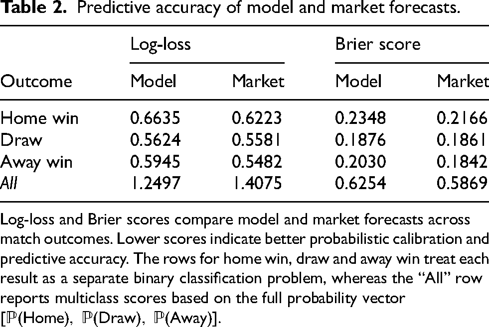
Log-loss and Brier scores compare model and market forecasts across match outcomes. Lower scores indicate better probabilistic calibration and predictive accuracy. The rows for home win, draw and away win treat each result as a separate binary classification problem, whereas the “All” row reports multiclass scores based on the full probability vector $[P (H o m e), P (D r a w), P (A w a y)]$ .

Model-based betting

Threshold ‘optimisation’

Although a forecast indicating positive expected value ( $E V > 0$ ) may appear sufficient to justify a bet, this is rarely reliable in practice. Small advantages are often indistinguishable from noise, and even modest model miscalibrations or market frictions can render such bets unprofitable. Furthermore, the choice of optimisation metric can affect the results – for example, prioritising total P&L over ROI.

Basic thresholds are introduced to determine empirically where potentially attractive bets can be found. They act as a form of practical ‘calibration’, narrowing the betting universe. Concretely, dynamic thresholds in a rolling-window setup are used. Based on information from an in-sample period – set again to two seasons here – the following filters are applied: a minimum expected value ${E V}_{m i n}$ , a maximum allowable odds level ${o d d s}_{m a x}$ and a minimum probability ‘edge’ $Δ p_{m i n}$ , where $Δ p : = p^{M o d e l} - p^{M a r k e t}$ . The rationale for applying these thresholds is to ensure that only sufficiently strong signals are considered: ${E V}_{m i n}$ filters out marginal bets with low expected return, ${o d d s}_{m a x}$ limits exposure to high-variance, low-probability outcomes, and $Δ p_{m i n}$ requires a material divergence between model and market views to act on perceived inefficiencies. Lastly, ${o d d s}_{m i n} = 1.25$ is imposed as a constant, avoiding the placement of bets with too low odds.

The betting opportunities are then scanned with the help of a grid search,³ and, individually for home, draw and away bets, the thresholds are tuned by varying ${E V}_{m i n}$ , ${o d d s}_{m a x}$ and $Δ p_{m i n}$ . Independent grid searches are carried out that aim for (a) the highest total P&L, (b) the highest ROI and (c) the highest Sharpe ratio. The search ranges over
${E V}_{m i n} \in {0.05, 0.10, \dots, 0.50},$
(6)
${o d d s}_{m a x} \in {1.50, 2.00, \dots, 10.00},$
(7)
$Δ p_{m i n} \in {0.05, 0.10, \dots, 0.25},$
(8)
yielding 900 parameter combinations for each outcome type and optimisation criterion. In order to mitigate overfitting, parameter combinations are only retained if they generate at least five qualifying bets within the calibration window. For each metric, the five best-performing parameter sets are then identified, the median value of each parameter across these is computed, and the actual parameter set is selected as the one closest to this median profile. Each criterion involves trade-offs: maximising P&L may favour high-variance outcomes, while Sharpe ratio optimisation can be overly sensitive to small sample volatility. The resulting optimised thresholds are used for the subsequent out-of-sample period. By rolling forward by one year each, this algorithm is continued across the entire study period.

Figure 5 illustrates the threshold optimisation process. For the example used, it is evident that the maximisation of the P&L aims for higher odds and thus greater potential payouts. For both ROI and Sharpe ratio, higher risk bets are constrained, however, as not commensurate with the optimisation goal.

Figure 5.
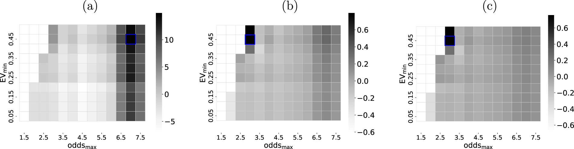
Illustration of grid search for parameter optimisation. On the example of home win bets within a single calibration window (2018/19 through 2019/20 seasons), the grid search for ‘optimal’ in-sample parameters across ${E V}_{m i n}$ and ${o d d s}_{m a x}$ is illustrated using heatmaps. The visualised ‘slices’ correspond to scenarios where the third parameter, $Δ p_{m i n} = 0.10$ , is held constant – although it remains part of the full grid search. The minimum odds threshold is fixed throughout at ${o d d s}_{m i n} = 1.25$ . The grid search targets three separate optimisation criteria: (a) highest total P&L, (b) highest ROI and (c) highest Sharpe ratio. The parameter combination yielding the optimal value is marked in blue.

Out-of-sample performance

The results from the rolling-window procedure and seasonal bet placements are summarised in Table 3. Performance metrics are reported only for season–outcome combinations with at least five qualifying bets (see also Section “Threshold ‘optimisation”’), to avoid overinterpreting very small samples. Depending on whether the in-sample optimisation targets the highest P&L, ROI or Sharpe ratio, the resulting out-of-sample performance differs noticeably.

Table 3.
Betting strategy – performance.

Bets Wins Win % Total P&L ROI Sharpe Max DD

A. Optimised for P&L

Home win 321 116 36.1% 54.25 16.9% 0.10 21.97

Draw 139 29 20.9% 17.33 12.5% 0.05 20.41

Away win 107 21 19.6% −17.73 −16.6% −0.09 36.63

All 567 166 29.3% 53.85 9.5% 0.05 41.09

B. Optimised for ROI

Home win 38 10 26.3% 3.78 9.9% 0.05 7.00

Draw 28 8 28.6% 13.79 49.3% 0.20 8.00

Away win 58 11 19.0% −10.40 −17.9% −0.10 23.79

All 124 29 23.4% 7.17 5.8% 0.03 16.68

C. Optimised for Sharpe

Home win 12 2 16.7% −7.20 −60.0% −0.63 7.26

Draw 20 6 30.0% 11.67 58.3% 0.23 7.00

Away win 32 9 28.1% 3.76 11.8% 0.06 9.62

All 64 17 26.6% 8.23 12.9% 0.06 10.41

D. Benchmark strategies

Hist. freq. 1,734 596 34.4% −144.56 −8.3% −0.05 178.86

Market fav. 2,754 1,447 52.5% −159.65 −5.8% −0.06 189.48

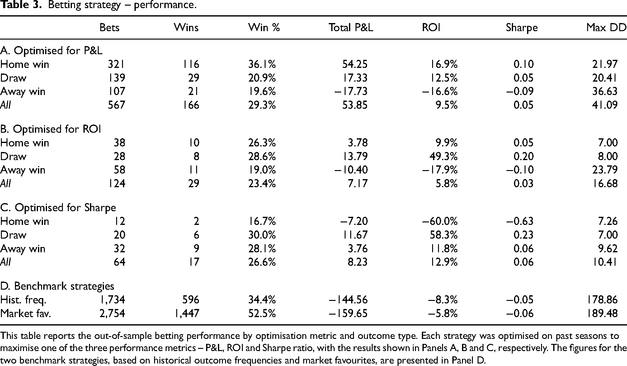
This table reports the out-of-sample betting performance by optimisation metric and outcome type. Each strategy was optimised on past seasons to maximise one of the three performance metrics – P&L, ROI and Sharpe ratio, with the results shown in Panels A, B and C, respectively. The figures for the two benchmark strategies, based on historical outcome frequencies and market favourites, are presented in Panel D.

When aiming for the highest P&L in the calibration phases (Panel A), the majority of the bets that are placed back home wins. About one-third of them are won and generate ca. 17% ROI. The inherent P&L volatility, however, renders the Sharpe ratio rather unattractive. Draw and away bets are placed less frequently and are successful in only around 20% of the cases. Backing away wins in particular is detrimental to the overall strategy and exhibits a standalone ROI of approximately -17%. In all three types of bets, the maximum drawdown (DD) suggests a rather high degree of instability across time, leading to periods of noticeable decreases in cumulative P&L. Overall, across all outcomes, a positive ROI remains – which would have been markedly higher if away bets were not to be placed.

The in-sample optimisation with respect to the highest ROI (Panel B) leads to substantially fewer placed bets. The overall ROI amounts to about 6% in this setup, still in conjunction with a very low Sharpe ratio. In line with this, even fewer bets are placed when targeting the highest Sharpe ratio during the in-sample grid search (Panel C). The very limited number of positions renders the resulting statistics not very insightful. The scarcity of the bets is driven by the very restrictive in-sample optimisation that, in many cases, tends to demand a large ${E V}_{m i n}$ or $Δ p$ . Such constellations – required for positive, low-volatility betting returns that can lead to an attractive Sharpe ratio – are not often encountered.

The two baseline strategies that place bets based on historical occurrence rates and market favourites, respectively, consistently lose money (Panel D), with ROI of -8% (historical frequency) and -6% (market favourite). Notably, despite a high win rate, the low odds on favourites result in a negative ROI owing to poor payout. This is in line with expectations, given that betting markets do not offer sustainable gains for uninformed bettors. As such, the simple model developed and tested here outperforms naive strategies.

Figure 6 visualises the cumulative P&L, additionally broken down by outcome type, on the example of an optimised in-sample grid search for the highest P&L. As seen in Table 3, the pattern is again clear: home win bets drive most gains, draw bets play a minor role, and away bets underperform.

Figure 6.
Cumulative P&L of betting strategy. The plot illustrates the cumulative P&L broken down by outcome type – home win, draw, away win – and aggregated across all bets (“All”). The results are based on optimising the in-sample parameter search for the highest P&L, i.e. aligned with Panel A in Table 3.

While the strategy evaluation abstracts from execution frictions, several real-world constraints should be noted. First, odds may not be available at meaningful volume, particularly for less liquid outcomes. Second, transaction costs such as spreads, commissions or slippage could erode profitability — especially at small edges or high turnover. Third, some bookmakers impose limits or account restrictions that may hinder systematic execution. These factors suggest that the reported returns represent an upper bound and should be interpreted as indicative of latent signal quality rather than readily realisable profits.

Robustness and sensitivity analysis

Season-by-season performance

Figure 7 illustrates the out-of-sample performance across individual Bundesliga seasons, on the example of the in-sample grid search optimised for the highest P&L. These results offer a more granular view of the overall performance patterns documented in Section “Results”, where pooled metrics indicate a certain profitability in terms of cumulative P&L.

Figure 7.
Season-by-season performance of betting strategy. This figure shows the P&L by season and outcome type – home win, draw, away win – and aggregated across all bets (“All”). The figures are based on optimising the in-sample parameter search for the highest P&L. Each bar shows the number of placed bets as additional information.

The generally high variability of the P&L over time is evident. Some seasons exhibit broad profitability (e.g. 2019/20), others underperform across the board. These fluctuations are consistent with the earlier findings in Section “Results”. The number of bets placed also fluctuates notably, despite the in-sample grid search spanning a period of two years. The picture is very similar for ROI and Sharpe ratio, and likewise when the in-sample optimisation explicitly targets those metrics (not shown here).

The pattern suggests that value opportunities in the market are inherently irregular or that the identification algorithm lacks sufficient specificity. Given a combination of sparse opportunity and high variance, systematically betting – at least under the current specification – is unlikely to be consistently profitable in the long run.

Parameter sensitivity

xG values: ‘calibration’ window

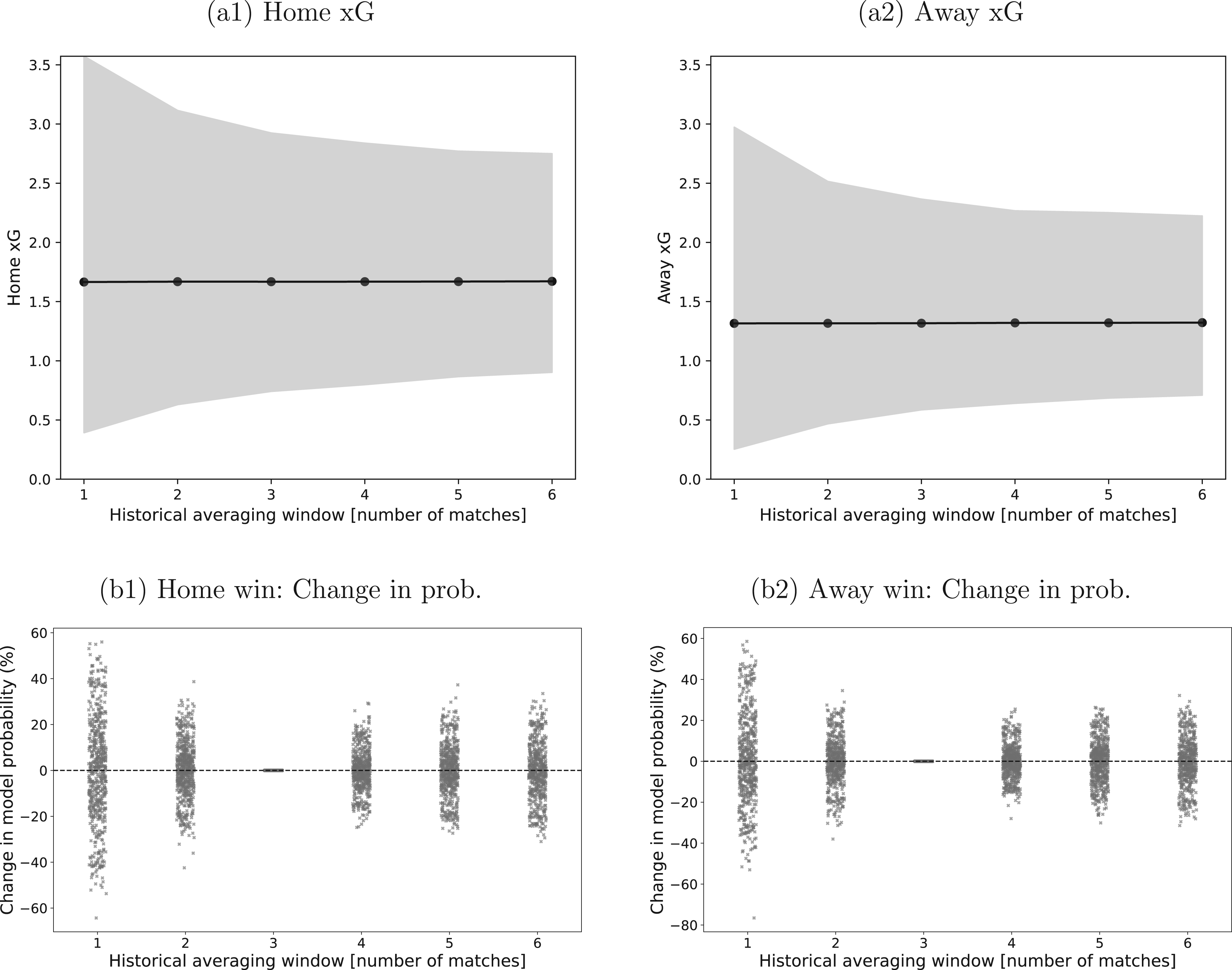
The estimation of the xG values is a crucial part of the modelling framework. The use of the average of the most recent $n = 3$ home or away matches is varied between $n \in {1, 2, \dots, 6}$ . Across the entire dataset, according to Figure 8, the averages are nearly unaffected. This implies that, at least on average, the probabilities for home wins, draws and away wins are also not sensitive to the estimation window for the xG values. As expected, the respective 90% confidence corridors for home and away xG are becoming narrower for increasing $n$ .

Figure 8.
Sensitivity of xG estimates and model probabilities to the historical estimation window. Panel (a1) shows the average xG for home teams across all matches as a function of the length of the historical averaging window $n$ . Panel (a2) presents the corresponding average xG values for away teams. The xG estimates are computed as rolling means over the previous $n$ venue-specific matches, as described in Section “Generating predictions from historical xG”. The grey-shaded areas represent the 90% confidence intervals. The resulting changes in probabilities for home wins and away wins, relative to the base case of $n = 3$ matches for the xG averaging, are provided in Panels (b1) and (b2).

When translating the xG averages into actual match probabilities, Figure 8 also provides the distribution of the differences over the base case. The majority of those are in the region of $\pm 20$ percentage points but can in extreme cases also reach $\pm 50$ percentage points. This means that the modelled outcome distribution can shift noticeably – in extreme instances even reversing the model-implied favourite.

The sensitivity of the ultimate profitability of the strategies to the xG determination (not shown here in detail) is moderate. For $n = 1$ , the total P&L amounts to $- 62$ ( $- 6$ % ROI), with home bets accounting for $- 16$ ( $- 3$ % ROI). With a shorter averaging period for the xG values, model probabilities (and hence betting opportunities) are available for more matches compared to the base case, whereas for $n = 6$ the opposite holds and coverage is reduced. In the case of $n = 6$ , the resulting P&L is equal to $- 14$ ( $- 4$ % ROI), whereby $+ 33$ ( $+ 15$ % ROI) stem from home bets. These results indicate that using only the most recent xG value for each team is insufficient for the model’s predictions. The absence of a clear trend or dominant performance across values of $n$ further suggests that – ceteris paribus – there is no universally optimal calibration window.

Odds: securing best ones in the market

The main results in Section “Out-of-sample performance” rely on the assumption that average market odds can be secured for all bets. This guarantees a certain liquidity and realistic execution setup. In an ideal case, bets could be placed at the best odds instead. The results of this modification – in comparison to the base case – are shown in Table 4.

Table 4.
Betting strategy – performance using average vs. best odds.

Bets Wins Win % Total P&L ROI Sharpe Max DD

I. Average odds

Home win 321 116 36.1% 54.25 16.9% 0.10 21.97

Draw 139 29 20.9% 17.33 12.5% 0.05 20.41

Away win 107 21 19.6% −17.73 −16.6% −0.09 36.63

All 567 166 29.3% 53.85 9.5% 0.05 41.09

II. Best odds

Home win 321 116 36.1% 72.31 22.5% 0.12 21.34

Draw 139 29 20.9% 24.69 17.8% 0.07 19.24

Away win 107 21 19.6% −12.78 −11.9% −0.06 33.75

All 567 166 29.3% 84.22 14.9% 0.07 39.17

This table reports the out-of-sample betting performance under flat stakes, comparing the use of average odds (Section I) and best available odds (Section II). Strategies were optimised for P&L.

Notably, the better odds are used for the actual bets but not for determining the betting decision itself; the latter are still based on the same grid search as before, to ensure that the trading ‘signal’ itself is robust enough. The P&L for backing away wins is still negative, but the total P&L is now substantially higher ( $84$ vs. $54$ ). The same is true for the ROI ( $15 %$ vs. $10 %$ ). The high P&L volatility (low Sharpe ratio) and considerable drawdown risk remain a concern even in this more optimistic scenario.

Money management strategy: fractional Kelly

Table 5 highlights the effect of fractional Kelly staking with $f = 0.50$ on out-of-sample betting performance relative to the previously described flat betting approach. Since only the staking is amended compared to the base case, the number of bets placed and won is identical in this scenario.

Table 5.
Betting strategy – performance across different money management strategies.

Bets Wins Win % Total P&L ROI Sharpe Max DD

I. Average odds

Home win 321 116 36.1% 54.25 16.9% 0.10 21.97

Draw 139 29 20.9% 17.33 12.5% 0.05 20.41

Away win 107 21 19.6% −17.73 −16.6% −0.09 36.63

All 567 166 29.3% 53.85 9.5% 0.05 41.09

II. Fractional Kelly ( $f = 0.50)$

Home win 321 116 36.1% 8.56 2.7% 0.11 2.36

Draw 139 29 20.9% 1.65 1.2% 0.09 1.16

Away win 107 21 19.6% −2.63 −2.5% −0.13 4.59

All 567 166 29.3% 7.57 1.3% 0.06 3.23

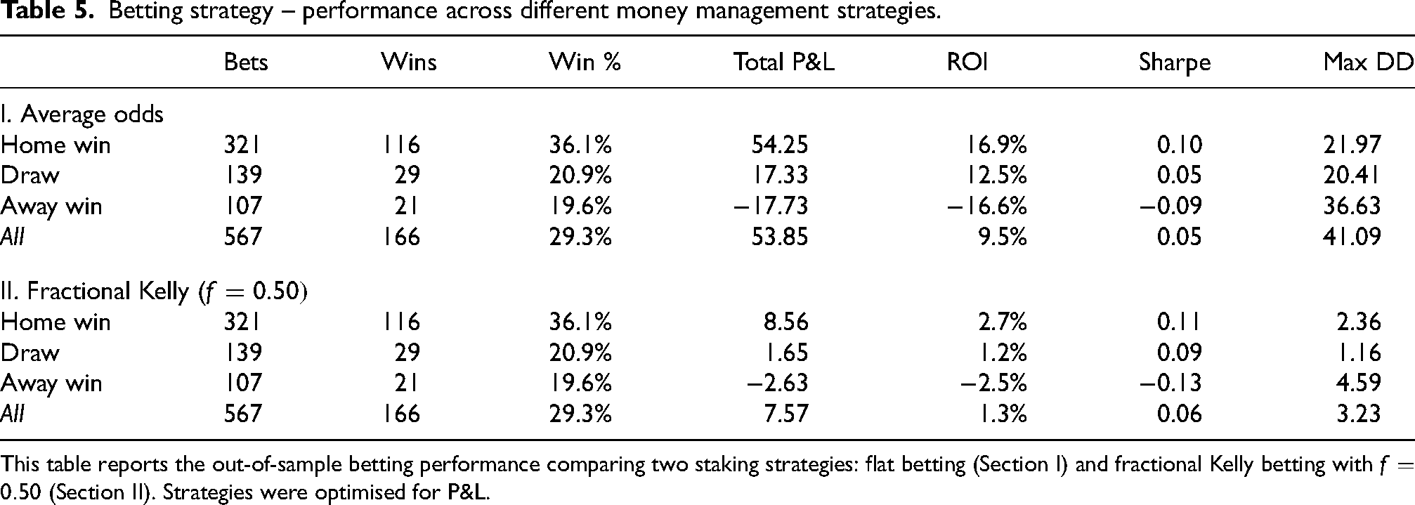
This table reports the out-of-sample betting performance comparing two staking strategies: flat betting (Section I) and fractional Kelly betting with $f = 0.50$ (Section II). Strategies were optimised for P&L.

The fractional Kelly method produces more moderate total profits and ROI, reflecting its more conservative stake sizing. Sharpe ratios remain low and close to those observed under flat betting, while maximum drawdowns exhibit a pronounced reduction, indicating improved capital preservation.

More adaptive approaches could further refine capital allocation. For example, dynamic Kelly schemes adjust $f$ based on recent performance volatility, drawdown constraints or uncertainty around the $E V$ estimate. Such strategies could offer improved risk control in volatile regimes or help preserve capital. At the same time, however, they also introduce additional complexity and calibration risk, which may counteract the simplicity and transparency goals of the current framework.

Impact of isotonic calibration

Finally, in order to gauge whether the positive ROI are driven primarily by the isotonic calibration layer or by the underlying xG-Skellam signal, the betting performance was recomputed with the isotonic regression step removed. With isotonic calibration, the main flat-stake strategy based on average odds achieves a total profit of about 54, corresponding to an ROI of roughly 10%. Without isotonic calibration, applying the same selection mechanism directly to the raw Skellam probabilities still produces a positive but much smaller profit of around 6, with an ROI close to 1%. The incremental gain from isotonic regression is therefore material, but the underlying xG-Skellam model already exhibits some predictive value on its own.

The cross-section of bets indicates that the main role of isotonic calibration is to trim poorly calibrated away-win positions. Without the additional step, away bets generate a strongly negative ROI of about $- 38$ % and substantial drawdowns; after applying isotonic regression, their loss rate moderates to roughly $- 17$ %, while home and draw bets remain broadly similar in number and performance. In this sense, isotonic regression primarily acts as a conservative filter on the most fragile part of the forecast spectrum, rather than as an independent source of profitability.

Conclusion and outlook

This paper evaluates whether simple, xG-based models can generate accurate and economically valuable football forecasts. Using a Skellam distribution to convert recent xG values – augmented by isotonic regression to improve forecast calibration – into match probabilities, the model is assessed across eleven Bundesliga seasons by comparing predictive accuracy and calibration to those of bookmaker-implied probabilities.

While market odds remain better calibrated, the xG-based model captures certain structural signals that translate into modest but consistent profitability in simulated betting, with the strongest performance observed for home win outcomes. Away bets tend to dilute returns. The isotonic calibration layer improves both reliability and profitability mainly by trimming poorly calibrated away-win positions, while robustness checks show that the underlying xG-Skellam probabilities already contain a modest positive signal on their own. Performance shows some robustness but varies across seasons and bet types. Alternative staking methods, such as fractional Kelly, help reduce drawdown risk but trade off against total return.

A natural next step would be to explore ensemble-style forecasts that combine model- and market-based probabilities. Since the model uncovers latent inefficiencies while markets offer strong calibration, blending the two could improve reliability and economic performance without sacrificing interpretability. Although this study abstracts from frictions such as slippage or betting limits, future work could simulate such effects to better approximate real-world execution. Similarly, while richer feature sets or dynamic inputs might improve accuracy, any such additions should be judged by whether they enhance usability without undermining the core strengths of simplicity, robustness and low model risk. In contrast to recent studies that employ complex machine learning architectures or context-aware expected points models (Bassek et al., 2025; Cavus and Biecek, 2022), this study deliberately prioritises structural parsimony and interpretability.

In summary, the analysis shows that simple, data-driven models – if well-constructed and properly filtered – can extract meaningful signals and, in some settings, deliver economically viable returns from football betting markets. As economist Tim Harford observed: “The power of a good model lies not in its complexity, but in its ability to illuminate.”

	Log-loss	Brier score
Home win	0.6635	0.6223	0.2348	0.2166
Draw	0.5624	0.5581	0.1876	0.1861
Away win	0.5945	0.5482	0.2030	0.1842
All	1.2497	1.4075	0.6254	0.5869

	Bets	Wins	Win %	Total P&L	ROI	Sharpe	Max DD
A. Optimised for P&L
Home win	321	116	36.1%	54.25	16.9%	0.10	21.97
Draw	139	29	20.9%	17.33	12.5%	0.05	20.41
Away win	107	21	19.6%	−17.73	−16.6%	−0.09	36.63
All	567	166	29.3%	53.85	9.5%	0.05	41.09
B. Optimised for ROI
Home win	38	10	26.3%	3.78	9.9%	0.05	7.00
Draw	28	8	28.6%	13.79	49.3%	0.20	8.00
Away win	58	11	19.0%	−10.40	−17.9%	−0.10	23.79
All	124	29	23.4%	7.17	5.8%	0.03	16.68
C. Optimised for Sharpe
Home win	12	2	16.7%	−7.20	−60.0%	−0.63	7.26
Draw	20	6	30.0%	11.67	58.3%	0.23	7.00
Away win	32	9	28.1%	3.76	11.8%	0.06	9.62
All	64	17	26.6%	8.23	12.9%	0.06	10.41
D. Benchmark strategies
Hist. freq.	1,734	596	34.4%	−144.56	−8.3%	−0.05	178.86
Market fav.	2,754	1,447	52.5%	−159.65	−5.8%	−0.06	189.48

	Bets	Wins	Win %	Total P&L	ROI	Sharpe	Max DD
I. Average odds
Home win	321	116	36.1%	54.25	16.9%	0.10	21.97
Draw	139	29	20.9%	17.33	12.5%	0.05	20.41
Away win	107	21	19.6%	−17.73	−16.6%	−0.09	36.63
All	567	166	29.3%	53.85	9.5%	0.05	41.09
II. Best odds
Home win	321	116	36.1%	72.31	22.5%	0.12	21.34
Draw	139	29	20.9%	24.69	17.8%	0.07	19.24
Away win	107	21	19.6%	−12.78	−11.9%	−0.06	33.75
All	567	166	29.3%	84.22	14.9%	0.07	39.17

	Bets	Wins	Win %	Total P&L	ROI	Sharpe	Max DD
I. Average odds
Home win	321	116	36.1%	54.25	16.9%	0.10	21.97
Draw	139	29	20.9%	17.33	12.5%	0.05	20.41
Away win	107	21	19.6%	−17.73	−16.6%	−0.09	36.63
All	567	166	29.3%	53.85	9.5%	0.05	41.09
II. Fractional Kelly ( $f = 0.50)$
Home win	321	116	36.1%	8.56	2.7%	0.11	2.36
Draw	139	29	20.9%	1.65	1.2%	0.09	1.16
Away win	107	21	19.6%	−2.63	−2.5%	−0.13	4.59
All	567	166	29.3%	7.57	1.3%	0.06	3.23

Footnotes

ORCID iD

Sascha Wilkens

Funding

The author(s) received no financial support for the research, authorship, and/or publication of this article.

Declaration of conflicting interests

The authors declared no potential conflicts of interest with respect to the research, authorship, and publication of this article.

Data availability

Historical xG data and betting quotes are freely available from Understat and Football-Data, respectively.

Notes

References

Baboota

Kaur

(2019) Predictive analysis and modelling football results using machine learning approach for English Premier League. International Journal of Forecasting 35(2): 741–755.

Bassek

Rein

Weber

, et al. (2025) An integrated dataset of spatiotemporal and event data in elite soccer. Scientific Data 12: 195.

Berrar

Lopes

Dubitzky

(2024) A data- and knowledge-driven framework for developing machine learning models to predict soccer match outcomes. Machine Learning 113: 8165–8204.

Bialkowski

Lucey

Carr

, et al. (2014) Identifying team style in soccer using formations learned from spatiotemporal tracking data. In: Proceedings of the IEEE International Conference on Data Mining Workshops (ICDMW), pp. 9–14. Shenzhen, China: IEEE.

Brechot

Flepp

(2020) Dealing with randomness in match outcomes: How to rethink performance evaluation in European club football using expected goals. Journal of Sports Economics 21(4): 335–362.

Brown

Yang

(2019) The wisdom of large and small crowds: Evidence from repeated natural experiments in sports betting. International Journal of Forecasting 35(1): 288–296.

Brown

Yang

(2021) Framing effects and the market selection hypothesis. Southern Economic Journal 88(1): 399–413.

Buchdahl

(2003) Fixed Odds Sports Betting: Statistical Forecasting and Risk Management. London: High Stakes Publishing.

Cameron

Trivedi

(1998) Regression Analysis of Count Data. Cambridge: Cambridge University Press.

10.

Cavus

Biecek

(2022) Explainable expected goal models for performance analysis in football analytics. In: 9th International Conference on Data Science and Advanced Analytics (DSAA), pp. 1–9. Shenzhen, China: IEEE.

11.

Constantinou

Fenton

Neil

(2013) Profiting from an inefficient association football gambling market: Prediction, risk and uncertainty in the Premier League. Knowledge-Based Systems 50: 60–86.

12.

Croxson

Reade

(2014) Information and efficiency: Goal arrival in soccer betting. The Economic Journal 124(575): 62–91.

13.

Dixon

Coles

(1997) Modelling association football scores and inefficiencies in the football betting market. Journal of the Royal Statistical Society: Series C (Applied Statistics) 46(2): 265–280.

14.

Dubitzky

Lopes

Davis

, et al. (2019) The open international soccer database for machine learning. Machine Learning 108: 9–28.

15.

Edalatpanah

Hess

(2024) Advancing football analytics: Predictive modeling and performance analysis in the Bundesliga using machine learning. Computational Engineering and Technology Innovations 1(4): 233–247.

16.

Egidi

Karlis

Ntzoufras

(2025) Predictive Modelling for Football Analytics. New York (NY): Chapman and Hall/CRC.

17.

Feng

Polson

(2016) The market for English Premier League (EPL) odds. Journal of Quantitative Analysis in Sports 12(4): 167–178.

18.

Fischer

Heuer

(2025) Match predictions in soccer: Machine learning vs. Poisson approaches. In: Memmert D (ed.) Artificial Intelligence and Machine Learning in Sports Science. Berlin/Heidelberg: Springer, pp. 91–102.

19.

Forrest

Goddard

Simmons

(2005) Odds-setters as forecasters: The case of English football. International Journal of Forecasting 21(3): 551–564.

20.

Franck

Verbeek

Nüesch

(2010) Prediction accuracy of different market structures: Bookmakers versus a betting exchange. International Journal of Forecasting 26(3): 448–459.

21.

Franke

(2020) Do market participants misprice lottery-type assets? Evidence from the European soccer betting market. The Quarterly Review of Economics and Finance 75: 1–18.

22.

(2024) Comparative analysis of expected goals models: Evaluating predictive accuracy and feature importance in European soccer. In: Proceedings of the 2nd International Conference on Machine Learning and Automation, Adana, Turkey.

23.

Goddard

Asimakopoulos

(2004) Modelling football match results and the efficiency of fixed-odds betting. Journal of Forecasting 23(1): 51–66.

24.

Groll

Kneib

Mayr

, et al. (2018) On the dependency of soccer scores – a sparse bivariate Poisson model for the UEFA European football championship 2016. Journal of Quantitative Analysis in Sports 14(2): 65–79.

25.

Hewitt

Karakus

(2023) A machine learning approach for player and position adjusted expected goals in football (soccer). Franklin Open 4: 100034.

26.

Hubacek

Sourek

Zelezny

(2019) Exploiting sports-betting market using machine learning. International Journal of Forecasting 35(2): 783–796.

27.

Hvattum

Arntzen

(2010) Using Elo ratings for match result prediction in association football. International Journal of Forecasting 26(3): 460–470.

28.

Joseph

Fenton

Neil

(2006) Predicting football results using Bayesian nets and other machine learning techniques. Knowledge-Based Systems 19(7): 544–553.

29.

Kain

Logan

(2014) Are sports betting markets prediction markets? Evidence from a new test. Journal of Sports Economics 15(1): 45–63.

30.

Karlis

Ntzoufras

(2003) Analysis of sports data by using bivariate Poisson models. The Statistician 52(3): 381–393.

31.

Karlis

Ntzoufras

(2009) Bayesian modelling of football outcomes: Using the Skellam’s distribution for the goal difference. IMA Journal of Management Mathematics 20(2): 133–145.

32.

Kaunitz

Zhong

Kreiner

(2017) Beating the bookies with their own numbers – and how the online sports betting market is rigged. Working paper, University of Tokyo.

33.

Kelly

(1956) A new interpretation of information rate. The Bell System Technical Journal 35(4): 917–926.

34.

Koopman

Lit

(2015) A dynamic bivariate Poisson model for analysing and forecasting match results in the English Premier League. Journal of the Royal Statistical Society: Series A (Statistics in Society) 178(1): 167–186.

35.

Kopriva

(2015) Constant bet size? Don’t bet on it! testing expected utility theory on Betfair data. Working paper, Charles University.

36.

Kozak

Glowania

(2021) Heterogeneous ensembles of classifiers in predicting Bundesliga football results. Procedia Computer Science 192: 1573–1582.

37.

Lambert

(1992) Zero-inflated Poisson regression, with an application to defects in manufacturing. Technometrics 34(1): 1–14.

38.

Lasek

Szlavik

Bhulai

(2013) The predictive power of ranking systems in association football. International Journal of Applied Pattern Recognition 1(1): 26–46.

39.

Maher

(1982) Modelling association football scores. Statistica Neerlandica 36(3): 109–118.

40.

Mead

O’Hare

McMenemy

(2023) Expected goals in football: Improving model performance and demonstrating value. PloS one 18(4): e0282295.

41.

Michels

Ötting

Karlis

(2025) Extending the Dixon and Coles model: An application to women’s football data. Journal of the Royal Statistical Society: Series C (Applied Statistics) 71(1): 167–186.

42.

Michels

Ötting

Langrock

(2023) Bettors’ reaction to match dynamics – evidence from in-game betting. European Journal of Operational Research 310(3): 1118–1127.

43.

Niculescu-Mizil

Caruana

(2005) Predicting good probabilities with supervised learning. In: Proceedings of the 22nd International Conference on Machine Learning (ICML), pp. 625–632. New York (NY): ACM.

44.

Ötting

Deutscher

Singleton

, et al. (2025) Betting on momentum in contests. Economic Inquiry 63(4): 1066–1089.

45.

Ötting

Langrock

Maruotti

(2023) A copula-based multivariate hidden Markov model for modelling momentum in football. AStA Advances in Statistical Analysis 107(1): 9–27.

46.

Ötting

Michels

Langrock

, et al. (2024) Demand for live betting: An analysis using state-space models. Applied Stochastic Models in Business and Industry 40(2): 527–541.

47.

Platt

(1999) Probabilistic outputs for support vector machines and comparisons to regularized likelihood methods. In: Smola AJ, Bartlett P, Schölkopf B and Schuurmans D (eds.) Advances in Large Margin Classifiers. Cambridge (MA): MIT Press, pp. 61–74.

48.

Robertson

Wright

Dykstra

(1988) Order Restricted Statistical Inference. New York (NY): John Wiley & Sons.

49.

Singh

Sharma

Kumar

, et al. (2025) The evolution of football betting: A machine learning approach to match outcome forecasting and bookmaker odds estimation. In: Saraswat M, Rajan A and Chakravorty A (eds.) Congress on Smart Computing Technologies. CSCT 2024. Smart Innovation, Systems and Technologies, Vol. 121. Singapore: Springer, pp. 117–130.

50.

Skellam

(1946) The frequency distribution of the difference between two Poisson variates belonging to different populations. Journal of the Royal Statistical Society. Series A (General) 109(3): 296.

51.

Strumbelj

(2014) On determining probability forecasts from betting odds. International Journal of Forecasting 30(4): 934–943.

52.

Stübinger

Knoll

(2018) Beat the bookmaker: Winning football bets with machine learning. In: Bramer M and Petridis M (eds.) Artificial Intelligence XXXV. SGAI 2018, Lecture Notes in Computer Science, Vol. 11311. Cham: Springer, pp. 219–233.

53.

Tippett

(2017) The Football Code: The Science of Predicting the Beautiful Game. Independently published.

54.

Tippett

(2019) The Expected Goals Philosophy: A Game-Changing Way of Analysing Football. Independently published.

55.

Tippett

(2024) xGenius: Expected Goals and the Science of Winning Football Matches. London: Bloomsbury Publishing.

56.

Uhrin

Sourek

Hubacek

, et al. (2021) Optimal sports betting strategies in practice: An experimental review. IMA Journal of Management Mathematics 32(4): 465–489.

57.

Vlastakis

Dotsis

Markellos

(2009) How efficient is the European football betting market? Evidence from arbitrage and trading strategies. Journal of Forecasting 28(5): 426–444.

58.

Wheatcroft

(2022) Evaluating probabilistic forecasts of football matches: The case against the ranking probability score. Journal of Quantitative Analysis in Sports 17(4): 273–287.

59.

Winkelmann

Deutscher

(2025) Do betting markets sense a goal coming? Evidence from the German Bundesliga. Working paper, University of Cologne.

60.

Winkelmann

Ötting

Deutscher

, et al. (2024) Are betting markets efficient? Evidence from simulations and real data. Journal of Sports Economics 25(1): 54–97.

61.

Wunderlich

Memmert

(2020) Forecasting the outcomes of sports events: A review. European Journal of Sport Science 20(3): 328–340.

62.

Xenopoulos

(2016) Using Skellam’s distribution to assess soccer team performance. Working paper, Pomona College.

63.

Zadrozny

Elkan

(2001) Obtaining calibrated probability estimates from decision trees and naive Bayesian classifiers. In: Proceedings of the 18th International Conference on Machine Learning (ICML), pp. 609–616. San Francisco (CA): Morgan Kaufmann.

64.

Zadrozny

Elkan

(2002) Transforming classifier scores into accurate multiclass probability estimates. In: Proceedings of the 8th ACM SIGKDD International Conference on Knowledge Discovery and Data Mining (KDD), pp. 694–699. New York (NY): ACM.

	Log-loss		Brier score
Outcome	Model	Market	Model	Market
Home win	0.6635	0.6223	0.2348	0.2166
Draw	0.5624	0.5581	0.1876	0.1861
Away win	0.5945	0.5482	0.2030	0.1842
All	1.2497	1.4075	0.6254	0.5869

Can simple models predict football — and beat the odds? Lessons from the German Bundesliga

Abstract

Keywords

Introduction

Previous research

Statistical modelling approaches

Market-based models and efficiency

Hybrid and machine learning approaches

Other approaches and supporting literature

Data and modelling framework

Data

Modelling framework based on expected goals

From xG to probabilistic forecasts

Generating predictions from historical xG

Model assumptions and simplifications

Model finetuning through isotonic regressions

Devising a betting strategy

Identification of value bets

Baseline strategies as benchmark

Historical frequency-based strategy

Market favourite strategy

Money management strategy

Results

Calibration and predictive accuracy

Model-based betting

Threshold ‘optimisation’

Out-of-sample performance

Robustness and sensitivity analysis

Season-by-season performance

Parameter sensitivity

xG values: ‘calibration’ window

Odds: securing best ones in the market

Money management strategy: fractional Kelly

Impact of isotonic calibration

Conclusion and outlook

Footnotes

ORCID iD

Funding

Declaration of conflicting interests

Data availability

Notes

References