Sage Journals: Discover world-class research

Abstract

This study develops a Monte Carlo simulation framework for estimating baseball offensive production using empirically derived event probabilities from play-by-play data. The model simulates complete innings and games to predict run distributions, player contributions, and lineup efficiencies. The proposed framework incorporates situational baserunning probabilities stratified by sprint speed categories, stolen-base attempts, double-play tendencies, and pitch-level outcomes, providing a comprehensive stochastic representation of offensive events. This approach uniquely integrates sprint-speed-conditioned baserunning transitions and lineup-level Monte Carlo optimization, achieving state-level fidelity not captured in prior Markov or aggregate simulators. Applications to multiple Major League Baseball (MLB) teams demonstrate the model's interpretability and potential for lineup optimization. Validation against multi-season empirical data confirms strong alignment between simulated and observed run distributions.

Keywords

baseball quantitative analysis run production modeling Monte Carlo simulation lineup optimization sprint speed

Introduction and background

The Major League Baseball (MLB) structure comprises 30 teams divided between the American and National Leagues. Each team plays 162 regular-season games, producing over 180,000 at-bats per season. Such a large event sample provides a robust empirical foundation for simulation-based modeling of offensive dynamics.

The quantitative analysis of baseball has long been a proving ground for the development of statistical and computational models. Early pioneers such as Lindsey (1963) demonstrated that strategies in baseball could be rigorously studied through operations research techniques, laying out the foundation for decades of simulation-based approaches. Subsequent works expanded these methods: Freeze (1974) applied Monte Carlo simulation to evaluate batting orders, while Cover and Keilers (1977) developed an “offensive earned-run average” that attempted to isolate the contribution of batting from contextual effects. These studies introduced the idea that baseball's complex sequences of events could be modeled probabilistically, capturing both chance and managerial strategy.

Markov chains became one of the most enduring approaches to modeling game dynamics. Bukiet et al. (1997) advanced a Markov chain framework to evaluate team performance, and later Davis (2011) applied Markov analysis to baseball board games, underscoring the versatility of state-based modeling. Kim (2018) extended this approach by developing higher-order Markov models, illustrating how additional memory in the chain could capture richer contextual dependencies in baseball outcomes. In parallel, Beaudoin (2013) demonstrated how simulators could incorporate more realistic baserunning and situational dynamics, building on his earlier explorations of probabilistic baseball modeling.

Monte Carlo methods have remained central to baseball simulation. In addition to Freeze’s (1974) early work, Sokol (2003) employed simulation-based heuristics to optimize batting orders under uncertainty. These techniques emphasized baseball's inherent stochasticity and the need for repeated sampling to estimate long-run tendencies. At the same time, Bayesian computation (Albert, 2006) and related inferential approaches provided a statistical foundation for updating player performance estimates, complementing simulation methods with principled probability modeling.

Researchers have also sought to reconcile baseball performance across contexts and eras. Berry et al. (1999) addressed the problem of comparing players from different periods, while Miller (2007) offered a mathematical derivation of the widely used Pythagorean win-loss formula. More recent work, including Baumer (2009), has refined estimates of baserunning impact, highlighting how specific in-game events contribute to overall team value.

Outside of academic journals, the rise of sabermetric communities has provided influential tools and perspectives. Tango, Lichtman, and Dolphin's The Book (2007) codified many of these insights into strategic principles, while Baseball Prospectus’ PECOTA system (n.d.) has become a widely used projection model. Retrosheet (2024) event files have enabled the large-scale empirical study of baseball outcomes, furnishing the data infrastructure necessary for simulation and statistical modeling.

Despite this rich body of work, most of the existing approaches face trade-offs between being realistic, transparent, and computationally efficient. Markov models offer elegant mathematical structures but often oversimplify situational dynamics such as baserunning. Subsequent developments in stochastic sports modeling (Lahvička, 2015; Percy, 2015; Schmanski, 2020; Steffen, 2020; Šarčević et al., 2021) have demonstrated the potential of Monte Carlo simulations to address these dependencies, particularly when parameterized with empirical event probabilities. These bodies of work illustrate both the progress and the persistent limitations of baseball simulation models—particularly their treatment of contextual dependencies such as baserunning.

This paper introduces a Monte Carlo simulation model that directly uses empirical event probabilities derived from Retrosheet play-by-play data. Unlike prior Markov approaches (Bukiet et al., 1997; Lin and Chen, 2008) that assume uniform transition probabilities, this model uses sprint-speed-stratified matrices, making it the first to empirically map advancement likelihoods to observed physical characteristics. In doing so, it offers a middle ground: as interpretable as Markov chain models, but as flexible as modern heuristic simulations, while grounded in empirical probabilities. By combining rigorous statistical tradition with scalable computation, this model advances the state of baseball simulation and provides a tool for both research and applied contexts in player evaluation and strategic decision-making. The model provides a transparent, extensible, and computationally efficient tool for baseball analytics. It allows researchers and practitioners to capture player-specific hitting and baserunning effects without sacrificing tractability, offering new insights for lineup optimization, player evaluation, and forecasting.

Methods

Overview

The proposed Monte Carlo simulation models offensive production by generating random sequences of plate appearances (PAs) according to empirically estimated event probabilities. Each simulated game consists of nine innings, with each inning continuing until three outs occur. Batter outcomes—single, double, triple, home run, walk, strikeout, groundout, and flyout—are drawn from the empirical probability distribution computed for each player.

The model further integrates situational baserunning transitions that depend on both the current base-out state and the sprint speed category of the runner. These transitions determine whether baserunners advance, hold, score, or are put out following each batted-ball event. Five speed categories (“very slow,” “slow,” “average,” “fast,” “very fast”) correspond to sprint speed thresholds of 25.3, 26.7, 27.7, 28.4, and 29.6 ft/s, reflecting the 5^th, 25^th, 50^th, 75^th, and 95^th percentiles, respectively. These thresholds correspond to empirical percentiles derived from Statcast sprint speed data (2015–2024), ensuring that baserunning dynamics reflect modern player mobility.

The simulation proceeds iteratively, updating the base-out state after each plate appearance. Runs scored, RBIs (Runs Batted In), and on-base events are accumulated at both player and team levels.

Data sources and preprocessing

Empirical event probabilities were computed using play-by-play data from Retrosheet. For each player, the frequency of singles, doubles, triples, home runs, walks, hit-by-pitch, strikeouts, flyouts, and groundouts was divided by total plate appearances to estimate outcome probabilities. Situational baserunning probabilities were also obtained from Retrosheet and stored in CSV files specifying the likelihood of scoring, advancing, or being out for every base-out combination. Situational probabilities were also computed for (1) double-play rates conditioned on the batter's speed, with opportunities defined as groundouts with a runner on first base and less than two outs, and (2) stolen-base and caught-stealing rates for runners on first and second, with opportunities defined per-batter plate appearance with the next base available for the baserunner. This data was computed using 40 players with sprint speeds within 0.1 ft/s of the given threshold across all available years of Statcast data (2015–2024). The chosen bandwidth balances local specificity with sufficient sample size, ensuring stable estimates even for rare base-out combinations. When applied to a given player, the probabilities were interpolated between adjacent sprint speed categories.

Justification of baserunning probability framework

The model parameterizes baserunning advancement through pooled empirical transition matrices stratified by sprint speed categories and interpolated for individual players. This approach balances empirical grounding with statistical stability. Direct estimation of player-specific advancement probabilities would require a prohibitively large sample for each base-out-event combination; pooling by speed percentile ensures that every transition probability is supported by sufficient observations while still reflecting a measurable physical determinant of baserunning ability. For a single full-time player (∼600 PA), many base-out-event combinations appear fewer than 5 times, which is far too small a sample size to capture the true value of the transition probabilities. The chosen approach ensures that every transition probability is derived from at least 50 opportunities, with most probabilities being drawn from 400 or more opportunities.

Beyond pragmatic sample-size considerations, there is a principled basis for centering sprint speed as the determinant for advancement probabilities. First, in a Statcast-era analysis of sac-fly situations, Kato and Yanai (2025) show that a runner's Sprint Speed materially shifts advancement outcomes from third even after accounting for batted-ball distance and context, deriving decision boundaries that move monotonically with measured speed. This is evidence that sprint ability operates as a primary physical constraint on advancement, not merely a correlate. Second, at the production-function level, Turocy (2005) demonstrates that adding footspeed to offensive models resolves omitted-variable bias and restores estimates consistent with game-theoretic equilibrium, implying that speed is a fundamental productive input distinct from tactical choices or small-sample outcomes (e.g., a player's limited stolen-base history). Taken together, these results justify pooling and interpolating advancement probabilities by measured sprint speed: it is (i) a biometric, high-reliability capacity that generalizes to small-sample players, and (ii) the dominant physical driver of non-steal baserunning transitions in aggregate. The overlayed plots in Figure 1 show a clear, monotonic speed gradient with mostly separated confidence intervals, supporting sprint speed as the primary capacity driver of non-steal baserunning and justifying speed-stratified pooling in the model. Linear interpolation between neighboring strata provides a first-order, monotone mapping from measured sprint speed to advancement rates while preserving the empirical ordering of strata. In an exploratory check, a smoother interpolation scheme (splines) never impacted any validation metric by more than one percent of its original value. Thus, the linear scheme is retained for transparency and simplicity, and a thorough examination of alternative smoothing methods is left to future work.

Figure 1.

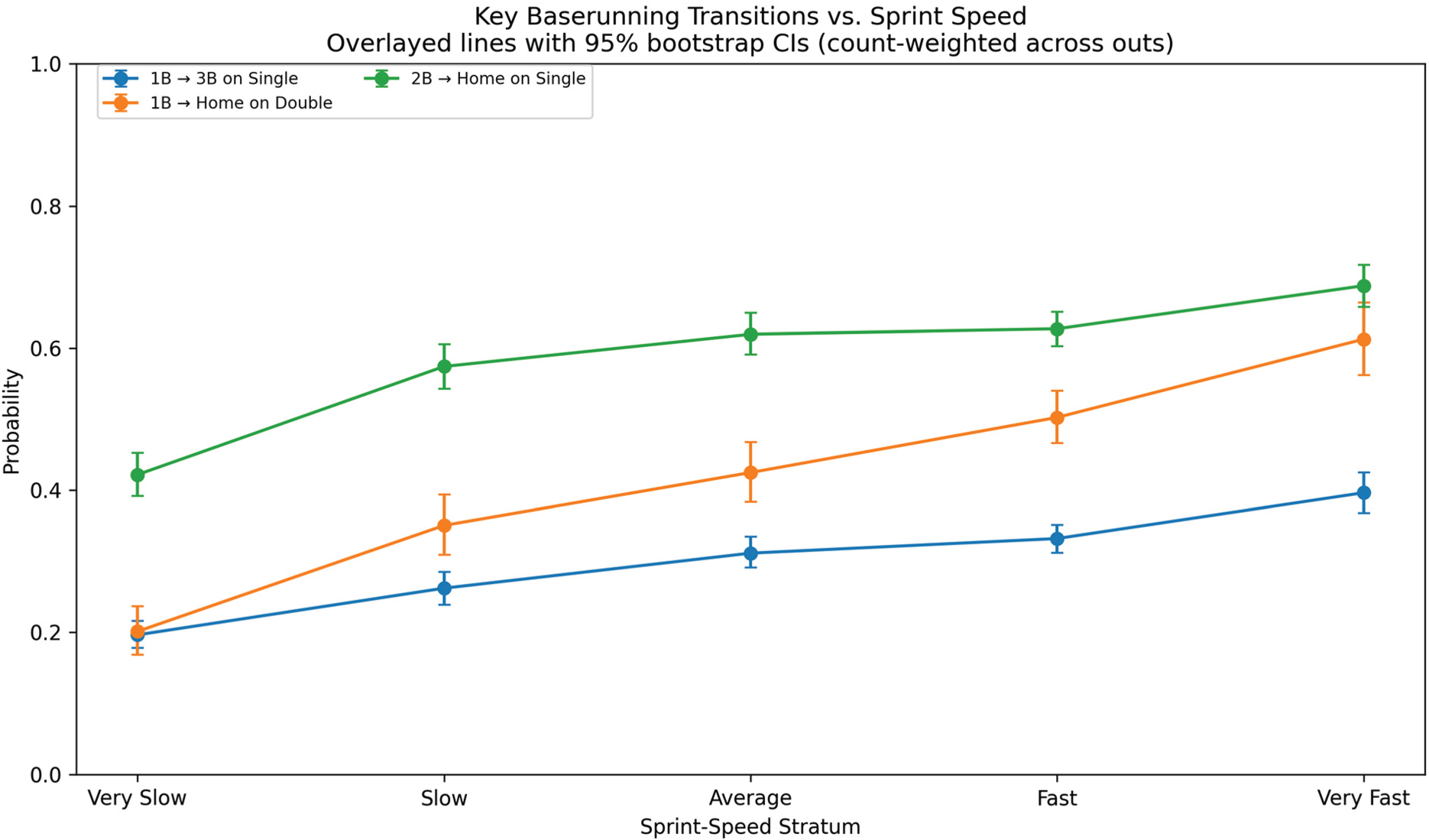
Key advancement probabilities vs. sprint speed stratum, derived from transition probability tables.

For stolen-base and caught-stealing modeling, the framework departs from the purely speed-based interpolation and instead applies a weighted average of individual player outcomes and probabilities pooled by sprint speed, where second base and third base opportunities are treated independently and weighted by batter plate appearances where the next free base for the runner is vacant. Because stolen-base opportunities and outcomes are both frequent and individually recorded, player-specific data provides low-variance estimates. Empirically, sprint speed explains only a modest fraction of variation in stolen-base success, which is strongly mediated by situational decision-making. Weighting individual rates by opportunity counts preserves the empirical distribution of stealing tendencies while ensuring that smaller sample-size cases are modeled in a manner that balances the variance of individual performance and bias of probabilities pooled by sprint speed. Operationally, the model weights linearly in the number of opportunities, with full individualization at K = 200 opportunities (w = min(n/K,1). The parameter K = 200 was chosen through a local search from K = 100 to K = 300 with a step size of 50, running the full validation diagnostics for each value of K and choosing the parameter that minimized the overall MSE (Mean Squared Error) for individual stolen-base and caught-stealing model predictions. This weighting scheme functions as a modified empirical-Bayes shrinkage and is mentioned for transparency; a comparative study of alternative shrinkage schedules for small-sample cases is left to future work.

Lastly, wild pitches are modeled using a fixed league-average probability per plate appearance with at least one runner on base. The wild pitch and passed ball rates are summed to one value, denoted WP, since these events have the same impact on baserunner advancement. Wild pitch events are sampled independently from stolen-bases and applied after stolen-base logic. Second-order effects, such as multiple stolen-bases or wild pitches in a single plate appearance, are neglected in this implementation due to their very low probability. The possible inclusion of such features, including highly anomalous events such as triple plays, is left to future work.

Together, these design choices reflect a guiding principle of the model: use individual data wherever sample size supports it, and resort to speed-stratified pooling where sparsity demands smoothing. This hybrid strategy intends to maximize both realism and statistical robustness while maintaining full transparency in how empirical inputs drive simulated outcomes. The modular construction of the baserunning component also ensures that data such as Statcast-level metrics for leads, jumps, or decision thresholds can be integrated seamlessly if necessary to enrich the behavioral realism of the advancement model. The resulting baserunning layer thus supplies empirically consistent advancement behavior to the simulation algorithms detailed below.

Simulation and optimization algorithms

This section details the Monte Carlo simulation pipeline used to generate offensive outcomes and lineup-optimization metrics. The procedure is decomposed into five algorithms:

− Algorithm 1 constructs player objects from observed event counts, sprint speed, and stolen-base data.

− Algorithm 2 simulates a single plate appearance (PA) given a player's outcome probabilities.

− Algorithm 3 simulates a half-inning by iterating plate appearances, applying the baserunning transition rules, and accumulating runs.

− Algorithm 4 stacks innings into full games to obtain game-level run totals.

− Algorithm 5 repeats game simulations to obtain season-level run distributions and player statistics, which are used for validation and lineup optimization.

Standard baseball notation is used throughout:

1B (single), 2B (double), 3B (triple), HR (home run), BB (walk), HBP (hit by pitch), SO (strikeout), FO (flyout), GO (groundout), PA (plate appearances), AB (at-bats), OBP (on-base percentage), SLG (slugging percentage).

All simulations were implemented in Python 3.11 on a desktop CPU (Intel i5, 32 GB RAM). Random numbers were generated using NumPy's Mersenne Twister implementation with a fixed random seed (seed = 162) for all reported results, ensuring exact reproducibility of validation outputs and illustrative figures. Exploratory runs with alternative seeds yielded differences only at the third decimal place in the reported validation metrics.

Algorithm 1. Player Initialization

Input: player-level event counts (1B, 2B, 3B, HR, BB, HBP, SO, FO, GO); sprint speed (ft/s); stolen-base and caught-stealing counts

Output: initialized Player object with outcome probabilities and baserunning parameters

Compute total plate appearances:

\begin{aligned} PA = & 1 B + 2 B + 3 B + HR + BB + HBP + SO \\ + FO + GO . \end{aligned}

Derive outcome probabilities for each event type (e.g., p(1B) = 1B / PA, p(2B) = 2B / PA, …, p(GO) = GO / PA).

Assign a sprint speed stratum k ∈ {1, …, 5} based on percentile thresholds [25.3, 26.7, 27.7, 28.4, 29.6] ft/s.

For the player's measured sprint speed, linearly interpolate baserunning advancement probabilities between the two adjacent strata bounding that speed (or use the nearest stratum if the speed lies outside the interior thresholds).

Estimate stolen-base and caught-stealing probabilities from the observed counts, applying empirical shrinkage (e.g., toward the league-average rate) for players with few attempts.

Store all outcome probabilities, baserunning parameters, and sprint speed information in the Player object.

Algorithm 2. Plate Appearance Simulation

Input: Player outcome probability vector

Output: event label in {1B, 2B, 3B, HR, BB, HBP, SO, FO, GO}

Draw a uniform random number u ∼ U(0, 1).

Construct the cumulative distribution function (CDF) over the player's outcome probabilities.

Find the smallest outcome index j such that CDF(j) ≥ u.

Return the corresponding event label (e.g., “1B”, “HR”, “SO”).

Algorithm 3. Inning Simulation

Input: lineup of 9 Player objects in fixed batting

order; starting batter index

Output: runs scored in the half-inning; updated batter index

Initialize:

outs ← 0

bases ← (empty configuration)

runs ← 0

b_idx ← starting batter index

While outs < 3:

Let batter ← lineup[b_idx].

Simulate a plate appearance:

event ← simul_PA(batter) (Algorithm 2).

Update base-out state:

Apply event-specific baserunning transition rules using the speed-stratified advancement probabilities associated with each runner (score, advance, or out). Transitions are sampled for lead runners first and are conditioned on both the event type and current base-out state.

For groundouts with a runner on first and fewer than two outs, apply double-play probabilities conditioned on both batter and runner speed before sampling other advancements.

When a runner crosses home plate, increment runs by 1.

Apply wild-pitch and stolen-base logic:

For eligible steal situations, sample stolen-base or caught-stealing events using the player-specific probabilities stored in the Player object. Update bases, outs, and runs accordingly.

If at least one runner is on base, draw a Bernoulli wild-pitch indicator with fixed league-average probability WP = 0.0338 per plate appearance; if a wild pitch occurs, advance eligible runners according to the standard rule (one base).

Increment batter index:

b_idx ← b_idx + 1; if b_idx > 9, set b_idx ← 1.

3. Return (runs, b_idx).

Algorithm 4. Game Simulation

Input: lineup of 9 Player objects; number of offensive innings n_inn = 9

Output: total runs scored in a simulated game

Initialize total_runs ← 0; b_idx ← 1.

For inning = 1 to n_inn:

(runs_in_inning, b_idx) ← simul_inning(lineup, b_idx) (Algorithm 3).

total_runs ← total_runs + runs_in_inning.

Return total_runs.

Algorithm 5. Season Simulation and Summary Statistics

Input: lineup of 9 Player objects; number of simulated games N

Output: average RPG (runs per nine offensive innings) and player-level statistics

Initialize an empty list RUNS.

For i = 1 to N:

total_runs ← simul_game(lineup) (Algorithm 4).

Append total_runs to RUNS.

Compute mean_RPG = average(RUNS).

Aggregate player-level statistics across all simulated games, including:

OBP = on_base / PA

SLG = total_bases / AB

Other rate and counting statistics as needed.

Return (mean_RPG, player_stats).

Algorithms 1–5 together implement a complete inning and season-level simulator capable of producing reproducible offensive outcomes under empirically grounded event mixtures and speed-stratified baserunning behavior.

Validation

Validation framework

The simulator is assessed over complete Major League Baseball seasons from 2022 through 2024 at both team and player resolution. Validation was started from the 2022 season to avoid additional difficulties in handling pitchers batting in the National League. The same season-specific inputs that drive the simulator are used in the validation environment: batter event frequencies, sprint speed for baserunning, and Retrosheet identifiers. Schedules, starting batting orders, line scores by inning, and official lengths of games are parsed from Retrosheet game logs. Player season totals for runs, runs batted in, stolen-bases, caught-stealing, games, and plate appearances are obtained from the MLB Stats API after linking Retrosheet retro identifiers to MLBAM identifiers with the Chadwick register. All external downloads are cached to comma-separated value files to ensure reproducibility.

For each team and season, the nine-player batting order for every game is reconstructed from the game log. A game is excluded only if any listed starter does not appear in the season's input tables. All other games are eligible and are simulated at the lineup level before aggregation to the team season. Monte Carlo effort is concentrated in proportion to the contribution of each lineup to the true season by allocating a frequency-weighted simulation budget.

s i m s (ℓ) = S \times g a m e s (ℓ)

This design reduces estimator variance for high-exposure lineups and yields season aggregates whose uncertainty is dominated by the groups that matter most.

A regulation-only baseline for actual scoring is derived from the same game logs. From the line score string, only the columns for innings one through nine are summed for the offense of interest in each game, which removes all extra-inning scoring while retaining the full schedule. This ensures that simulated games correspond exactly to nine-inning scoring opportunities, eliminating confounds from extra-inning variance, such as runners automatically starting each extra inning at second base. The offensive innings batted in regulation are computed from the official length in outs (which can vary from 8 to 9 innings). Let $R_{i}^{r e g}$ denote regulation runs for game i and $I_{i}^{r e g}$ denote regulation offensive innings for that game. The season-level target is the ratio estimator shown below.

R P G_{a c t u a l^{r e g}} = \frac{\sum_{i} {R_{i}}^{r e g}}{\sum_{i} {I_{i}}^{r e g}} \times 9

The simulator produces a corresponding season quantity, $R P G_{s i m}$ , by weighting lineup-level simulated scoring with lineup game frequencies. The primary team-level error is defined as follows.

Δ_{t e a m} = R P G_{s i m} - R P G_{r e g}^{a c t u a l}

Two dispersion summaries accompany this error. The first is the empirical standard deviation of simulated RPG obtained from the pooled set of simulated games after weighting by lineup frequency. The second is the empirical standard deviation of actual game scoring from the logs, computed either on total runs or on regulation-only runs to mirror the baseline. Their difference quantifies whether the simulator is sharper or broader than observed variability.

Player-level validation uses the same lineup-weighted simulations. For each player-season combination, simulated totals of runs, runs batted in, stolen-bases, and caught-stealing are accumulated across all simulated games in which the player appears. Actual totals are retrieved from the MLB Stats API and summed across team stints if a player was traded, so that each record represents one player's season. To compare skill rather than opportunity, statistics are normalized by the player's real plate appearances. Let S be a simulated total, A the actual total, and PA the real plate appearances for that season. The per-plate appearance difference and its per-600-plate appearances scale are shown below.

δ_{p e r - P A} = \frac{S}{P A} - \frac{A}{P A}

Δ_{p e r - 600} = 600 \times δ_{p e r - P A}

A workload filter is applied to stabilize the comparison, typically four hundred plate appearances.

Two team-level graphics and three player-level graphics summarize performance. The scatter of simulated versus actual team scoring (Figure 2) places each team season against the identity line, with labels applied to the largest absolute residuals. The heat map by team and season (Figure 3) renders ΔRPG as a matrix to reveal persistent over or under-prediction for specific franchises or seasons. Player results are shown as simulated versus actual rates per six hundred plate appearances for runs (Figure 4), runs batted in (Figure 5), and stolen-bases (Figure 6). Points close to the identity line indicate that the simulator's event mixture and baserunning rules reproduce the player's realized season context after accounting for workload.

Figure 2.

Team simulated vs actual RPG (regulation).

Figure 3.

Heat map of team Δ (Sim − Actual RPG) by season.

Figure 4.

Player Runs per 600 PA: simulated vs actual.

Figure 5.

Player RBI per 600 PA: simulated vs actual.

Figure 6.

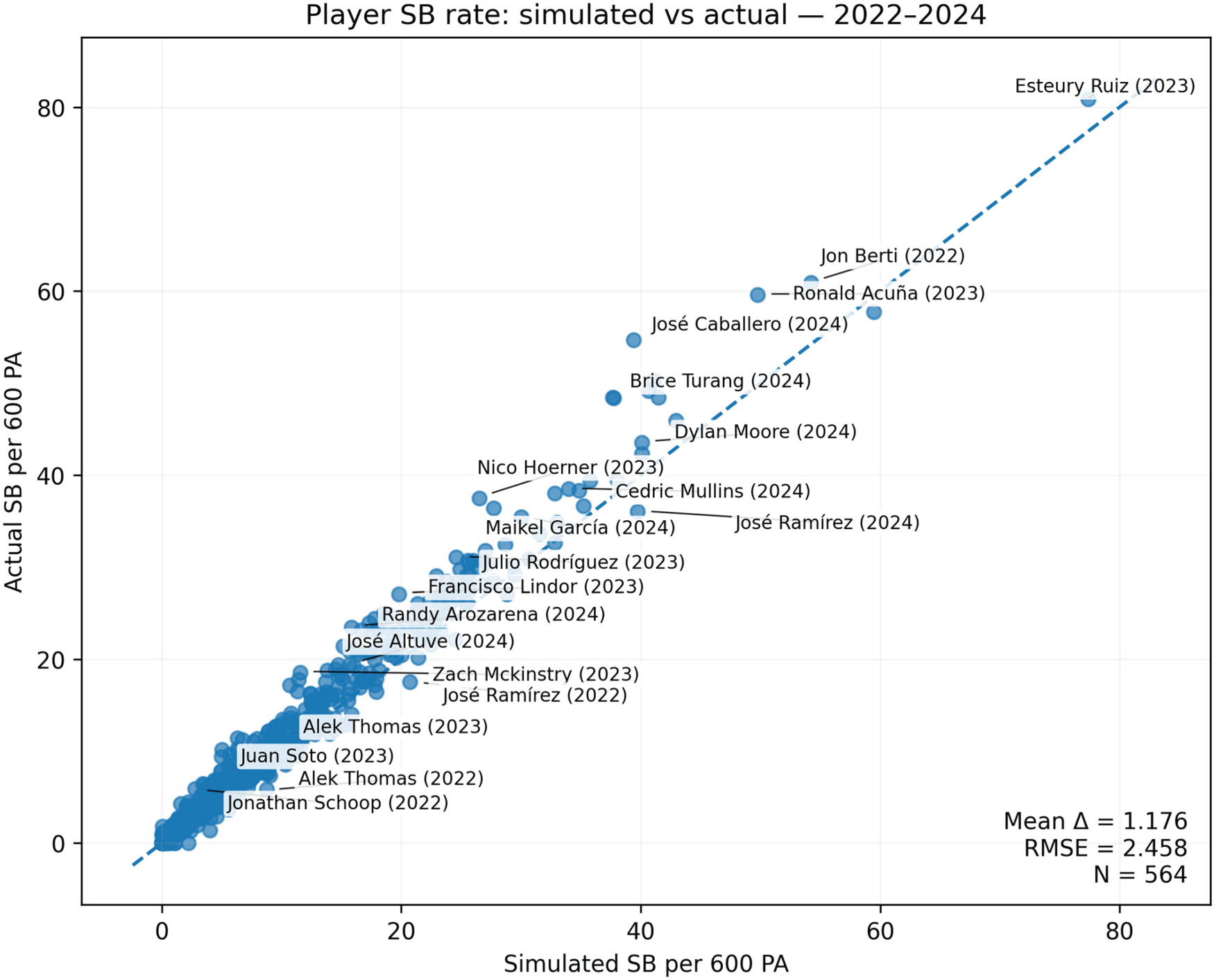
Player stolen-bases per 600 PA: simulated vs actual.

This validation design provides three methodological advantages. First, the simulation budget is aligned with lineup exposure, which produces precise season aggregates without oversampling rarely used orders. Second, the regulation-only baseline removes extra-innings scoring while preserving every game, which aligns the target with a nine-inning simulator and retains the club's true opponent and park mixture. Third, player comparisons are made on a common rate basis after summing across stints, which eliminates confounding from traded players and turns playing-time differences into transparent differences in per-plate appearance performance. Together with the diagnostic figures, this framework quantifies bias and dispersion at the team level and identifies the specific players and components where the simulator systematically over or undershoots, while remaining fully reproducible from cached public sources.

Statistical methods overview

The validation covers seasons 2022–2024 and treats simulated outputs as point forecasts of realized outcomes. Evaluation is organized around three complementary questions. First, average accuracy asks how far, on average, forecasts are from reality. Root-mean-squared error (RMSE), mean absolute error (MAE), and mean bias (actual minus simulated) are reported in the original units (RPG for teams, per-600 plate appearances for players). RMSE emphasizes larger errors relative to MAE. Second, calibration asks whether forecasts are unbiased and on the correct scale across the range. This is tested with the Mincer-Zarnowitz regression, y = α + βx, where ideal calibration implies α = 0 (no intercept bias) and β = 1 (correct spread) Mincer and Zarnowitz, 1969. Individual t-tests assess each restriction, and a joint Wald F-test assesses both simultaneously. Slopes with β < 1 indicate over-dispersion (extremes forecast too extreme) and β > 1 indicate under-dispersion (forecasts too conservative). For deployment, a simple post-hoc linear recalibration, $\hat{y} = \hat{α} + \hat{β} x$ , can realign the mean and scale based on historical data. Third, agreement and error structure are addressed with Lin's concordance correlation coefficient (CCC), which combines correlation and calibration penalties and equals 1 only under perfect correlation, zero bias, and correct scale; uncertainty is summarized with a bootstrap 95% confidence interval Lin, 1989 Efron and Tibshirani, 1994. Bland-Altman analysis reports the average difference and 95% limits of agreement (LoA) for individual observations Bland and Altman, 1986. Because LoA assumes approximately normal differences, Shapiro-Wilk is used to check that assumption, and LoA are interpreted descriptively where normality is rejected Shapiro and Wilk, 1965. A residual-trend check based on Spearman correlation between residuals and predictions is also reported to detect systematic error across the forecast range Spearman, 1904. For run scoring distributions, Wasserstein distance simply sums all of the CDF (Cumulative Distribution Function) differences, while the Kolmogorov-Smirnov (KS) statistic reports the largest CDF difference. All technical terms and their meaning are outlined in Appendix 6, and all results below reflect the 2022–2024 data filters.

Team-level validation

Team scoring (RPG) shows strong accuracy and agreement: RMSE = 0.162, MAE = 0.130, and mean bias = + 0.045 RPG, with a Pearson r of 0.956 and a CCC of 0.951 (95% CI: 0.922–0.968). Calibration is nearly ideal— $\hat{α}$ = 0.038 (p = 0.797) and $\hat{β}$ = 1.001 (p = 0.967)—although the joint Wald test rejects at the 5% level (F = 3.45, p = 0.036), indicating a very small but detectable multivariate departure from perfect calibration that is consistent with the modest positive mean bias. Bland-Altman shows a mean difference of +0.045 and LoA [−0.263, 0.353]. RPG normality is not rejected (Shapiro-Wilk p = 0.899), and residuals exhibit no trend across the prediction scale (Spearman p = 0.901). Figure 3 visualizes these team-level residuals as a heat map of Δ(Sim − Actual) by club and season; nearly all cells fall within approximately ±0.20 RPG, with only a small number of isolated deviations approaching ±0.40 RPG. Crucially, there are no pronounced vertical (season-specific) or horizontal (team-specific) bands of red or blue—positive and negative residuals are scattered idiosyncratically across franchises and years—suggesting that remaining errors are small and context-specific rather than structural. In practical terms, team forecasts are highly accurate and close to perfectly calibrated, with a slight tendency to underpredict scoring by roughly 0.045 RPG. Overall, the team model achieves very high agreement and near-ideal calibration, with a minor positive bias that can be removed with a trivial adjustment of the intercept if desired.

Player-level validation

Runs (R per 600 PA)

Accuracy and agreement are strong given player-level variability (RMSE = 7.03, MAE = 5.67, bias = + 0.402, r = 0.833, CCC = 0.826 with 95% CI 0.794–0.851). Calibration indicates over-dispersion: $\hat{α}$ = 4.934 (p = 0.012), $\hat{β}$ = 0.938 (p = 0.020), and joint F = 3.66 (p = 0.026), meaning forecasts at the extremes are too extreme relative to realized values. A linear recalibration modestly improves error (RMSE 6.98, MAE 5.64) and removes mean bias by construction. Bland-Altman shows a mean of +0.402 with wide LoA [−13.37, 14.17]; differences depart from normality (Shapiro-Wilk p = 0.015), so LoA are descriptive.

RBI (RBI per 600 PA)

Accuracy and agreement remain high (RMSE = 8.02, MAE = 6.28, bias = + 1.436, r = 0.877, CCC = 0.867 with 95% CI 0.842–0.887). The Mincer-Zarnowitz regression yields $\hat{α}$ = 2.088 (p = 0.203) and $\hat{β}$ = 0.991 (p = 0.685), yet the joint Wald test rejects (F = 9.40, p < 0.001), a pattern consistent with mild multivariate miscalibration when α and β are correlated. Recalibration produces modest gains (RMSE 7.89, MAE 6.23). Bland-Altman indicates a mean of +1.436 with LoA [−14.04, 16.91]; differences are non-normal (Shapiro-Wilk p = 0.029).

Stolen-bases (SB per 600 PA)

Predictability is especially high (RMSE = 2.46, MAE = 1.57, bias = + 1.176, r = 0.987, CCC = 0.974 with 95% CI 0.968–0.980). Calibration shows under-dispersion: $\hat{α}$ = 0.126 (p = 0.246), $\hat{β}$ = 1.109 (p < 10⁻³), with joint F = 211.77 (p < 10⁻³), indicating forecasts vary too little compared with realized outcomes. Recalibration materially improves accuracy (RMSE 1.86, MAE 1.29). Bland-Altman yields a mean of +1.176 and LoA [−3.06, 5.41]; differences are strongly non-normal (Shapiro-Wilk p ≈ 7.2 × 10⁻²²), so LoA are again descriptive.

At the player level, the Runs and RBI categories show mild over-dispersion (β < 1) and benefit slightly from shrinkage via linear recalibration, while stolen-bases exhibit under-dispersion (β > 1) and benefit from an expanded forecast spread, with a corresponding improvement in accuracy. The non-normality of the runs and RBI deltas (Shapiro-Wilk p < 0.05) can be attributed to differences in the number of plate appearances in the real data, which would lead to inconsistent variance in player production statistics, such as runs and RBIs. A test that limited the real PA range to 400–450 yielded a Shapiro-Wilk p of 0.434 and 0.422 for runs and RBIs, respectively, demonstrating that reducing the variance in plate appearances resolved non-normality of the real-to-simulation deltas. For stolen-bases, the high CCC and low Shapiro-Wilk p suggest that differences are small but systematic.

Distributional validation

The first panel plots, for each team-season from 2022 to 2024, the one-dimensional Wasserstein distance between the simulated and empirical run distributions against the Kolmogorov-Smirnov (KS) statistic. The points form a clear increasing curve: cases with small KS gaps tend also to have small transport distances, while the largest KS values (≈0.08–0.09) coincide with the largest Wasserstein values (≈0.45–0.50). Because KS emphasizes the single largest CDF discrepancy and Wasserstein aggregates how far probability mass must be shifted to match the empirical distribution, their joint rise indicates that disagreements tend to involve both localized shape errors and broader location/scale displacement rather than being confined to one aspect of the distribution. Most team-seasons cluster around KS ≈0.03–0.06 and Wasserstein ≈0.15–0.35, consistent with generally close agreement and a minority of contexts that merit targeted calibration. The pattern suggests that model misspecification, when present, is primarily scale-related rather than structural, a correctable form of dispersion error (Figures 7 and 8).

Figure 7.

Wasserstein vs KS for all team, year pairs from 2022 to 2024.

Figure 8.

Aggregate team run scoring probability mass function: simulated vs. real.

The second figure reports the aggregate scoring frequencies for both simulation and real scoring data. The pattern is systematic. A negative residual at 0 runs indicates that the simulator assigns too little mass to very low-scoring games. Positive residuals from roughly 2 to 9 runs show compensating overweights in the midrange of the distribution, as small negative residuals reappear from 10 runs onwards. Taken together, these diagnostics imply a modest under-dispersion in the simulated team run distributions: probability is pulled from the tails and pushed into common midrange scores. These diagnostics also give relevance to the observed disparity in the overall distribution mean, where the simulation underestimates real scoring by a modest 0.024 runs. A systematic underdispersion, rather than a distribution shift, is the root cause of the observed disparity in means. This implies that small parameter tweaks that lead to systematically more scoring in the simulation would not be sufficient to match the simulated and real run-scoring probability mass functions.

Unlike recent offensive simulators that evaluate realism primarily by matching a single league-wide mean or by validating micro-level event probabilities, the present study conducts a season-scale, distribution-aware validation across all MLB teams (2022–2024). The model attains RMSE = 0.162 and MAE = 0.130 RPG with r = 0.956 and CCC = 0.951, near-ideal calibration in a Mincer-Zarnowitz test, and tight Bland-Altman limits; it also quantifies distributional fidelity with KS and 1-Wasserstein distances and reports interpretable tail probabilities. Prior work either compares only means without formal testing—e.g., 4.27 simulated vs 4.22 actual RPG in NPB (Nippon Professional Baseball) with no KS/Wasserstein or CIs (Nakahara et al., 2023)—or validates event-level probabilities (e.g., MSE 0.0644→0.0398 with defense; Doo and Kim, 2018) rather than season-level game outcomes. Classic Markov approaches have also shown significant systematic underprediction (≈6.7% fewer runs; Bukiet et al., 1997). Taken together, these contrasts support the claim that this model represents real offensive outcomes more faithfully than recent alternatives, not merely in expectation but across the full run distribution with documented calibration and uncertainty.

Applications: A lineup optimization algorithm

To illustrate the simulator's applied utility, a lineup-ordering experiment was conducted. The simulator is applied to a single team-year to examine whether the batting order, holding the nine everyday players fixed, materially changes simulated RPG. The scope is limited to ordering only so that the example isolates the contribution of the simulation framework.

The case study considers the Philadelphia Phillies’ 2024 season. Nine players meeting a usage threshold are fixed. The baseline lineup is the modal as-played order for those nine when appearing together; candidate lineups are permutations of the same nine players. All other inputs—event-level probabilities, baserunning matrices, and stolen-base/double-play risks—are held constant. For each lineup, the primary outcome is RPG (mean with 95% confidence interval). Distributional changes are summarized with the Kolmogorov-Smirnov (KS) statistic, the 1-Wasserstein distance on full-game run totals, and the change in the upper-tail probability P(runs ≥ 6). PMFs and statistics are estimated from 100,000 simulated games per lineup.

Candidate orders are explored using a lightweight genetic-style local search intended solely as a proof of concept. Each epoch evaluates the current population of lineups with N simulated games per lineup. Offspring are generated by swaps that are (i) global in early epochs (random non-adjacent pair) and (ii) local after ≈30% of epochs (adjacent swaps) to refine promising orders. An offspring is retained only if its estimated RPG exceeds its parent by an annealed margin δ_i = δ₀·(1 + i/E), with δ₀ = 0.02, epoch index i, and total epochs E. Scores are cached and combined across epochs to reduce Monte Carlo variance when a lineup is revisited. Hyperparameters for the run shown here: initial variations = 500; intended population size = 20; epochs = 60; offspring per parent = 1 with probability 0.9; N per lineup per epoch = 1000 initially and ≈3000 in later epochs (growth rate = 1.0). There is no stopping condition in the algorithm as the number of epochs is specified by the user, but at around 30–40 epochs, the average production of the best lineups tended to plateau for trial runs. The heuristic is not claimed as a contribution; it is included only to illustrate how the simulator can be used to compare batting orders. Detailed pseudocode of the lineup optimizer heuristic can be found in the appendix.

Lineups compared (1→9):

Baseline: Kyle Schwarber; Trea Turner; Bryce Harper; Alec Bohm; J. T. Realmuto; Brandon Marsh; Nick Castellanos; Bryson Stott; Johan Rojas.

Selected (algorithm): Kyle Schwarber; Brandon Marsh; Bryce Harper; Nick Castellanos; J. T. Realmuto; Bryson Stott; Trea Turner; Johan Rojas; Alec Bohm.

For each lineup, RPG is the sample mean over simulated games; 95% confidence intervals use a nonparametric bootstrap (1000 resamples). The baseline vs. selected comparison reports ΔRPG and a bootstrap CI for the difference. KS and 1-Wasserstein quantify distributional differences; P(runs ≥ 6) is reported for interpretability (Figure 9).

Figure 9.

Run scoring probability mass function for most common and algorithm-selected 2024 Phillies lineups with the same players.

The selected lineup increases mean RPG from 5.102 [5.083, 5.123] to 5.178 [5.157, 5.200], a difference of ΔRPG = 0.076 [0.046, 0.105], where confidence intervals are based on bootstrapped RPG means. The full-game run distributions are very similar (KS = 0.009, W₁ = 0.076 runs), with a small but directionally consistent increase in upper-tail probability P(runs ≥ 6) from 0.395 to 0.404. As expected for order-only changes among the same nine players, the gains are modest. The optimization agreed with placing Kyle Schwarber in the leadoff spot, a decision considered controversial by classical lineup construction methodology, which typically places the most productive hitters in the 3^rd or 4^th lineup spot. It was only a handful of swaps in the later order that caused a small improvement of 0.076 RPG, which would amount to roughly 12 runs in a 162-game season. While modest, this gain aligns with the expected order of magnitude for realistic lineup adjustments, supporting the simulator's practical sensitivity.

The example excludes platoon-based substitutions and pitcher-dependent probabilities and uses a simple local search with annealed acceptance. Optimizer design is orthogonal to the paper's main contribution; richer policies (e.g., learned proposals or Bayesian optimization) are left to future work. The value is to demonstrate that the simulator yields actionable, uncertainty-aware outputs.

Future work

Several extensions follow directly from the present design and would deepen both methodological rigor and applied utility. First, integrating richer Statcast features—such as primary and secondary leads, jump, and home-to-first splits—into the baserunning transition matrices would allow advancement to vary continuously with observed pre-pitch and on-contact behavior rather than only by sprint speed strata. Because advancement in the simulator is already governed by empirical, situational transition tables, these additions constitute a modular change to the data layer rather than a rewrite of the engine. Second, the framework can be used to evaluate families of baserunning decision rules that encode different levels of aggressiveness (e.g., send/hold thresholds and steal attempts as functions of outs, run environment, and arm strength). By holding batter outcomes fixed and altering only decision policies, the model can isolate whether and when a more aggressive approach yields tangible gains in run production. Third, the lineup search can be formalized with an optimizer whose behavior is specified a priori—e.g., simulated annealing with an explicit temperature schedule, the cross-entropy method, or Bayesian optimization over permutations—accompanied by principled stopping rules, variance control via common random numbers or caching, and sensitivity analyses that justify the choice of hyperparameters.

The same engine also enables team-building counterfactuals at the player level. Two-sided trade proposals can be assessed by simulating both clubs before and after the exchange, allowing effects to be computed in each club's park, league, and lineup context and summarized on the runs (or wins) scale. Player value can be made team-specific by direct replacement: substituting a role-appropriate, replacement-level hitter and measuring the change in team RPG quantifies contextual offensive value without invoking external metrics. Finally, the pure contribution of speed can be quantified through targeted perturbations—reassigning sprint speed percentiles or varying lead/jump inputs while holding contact quality and plate outcomes constant—to trace its effect on double-play avoidance, extra bases taken, and stolen-base risk. In all cases, the simulator's design—complete-inning Monte Carlo with explicit base-out transitions, empirical event probabilities, modular inputs, and cached estimates—makes these studies straightforward to implement and statistically auditable.

Conclusion

This study presents a transparent, empirically grounded simulation that reproduces team scoring distributions and supports uncertainty-aware comparisons on the runs scale. The contribution is a reliable evaluation engine: given any candidate policy—batting order, baserunning strategy, player swap, or contextual replacement—the model returns stable distributional estimates that can be validated, contrasted across alternatives, and summarized for decision-making. Because each component (event probabilities, advancement rules, and decision policies) is data-addressable and separable, the framework is well-positioned for integration of richer Statcast features and for adoption of formal optimization methods. Taken together, these properties make the simulator a practical bridge between academic methodology and baseball operations, enabling future work that is both statistically rigorous and operationally actionable. In doing so, it demonstrates that empirical Monte Carlo frameworks can serve as transparent alternatives to proprietary projection systems.

Although the simulator captures the principal physical and probabilistic determinants of offensive production, several behavioral and contextual dimensions remain simplified. Runner decisions, for example, depend not only on sprint speed but also on lead length, jump timing, ball trajectory, fielder positioning, and coaching aggressiveness. These influences are therefore represented implicitly, through their historical imprint on event probabilities, rather than explicitly as controllable parameters. Incorporating such variables directly would increase model realism but also fragment the sample space: as more parameters are introduced, the number of observations supporting each conditional probability decreases, potentially raising variance faster than bias declines. To balance realism and statistical stability, the current design limits the baserunning model to a single, continuous physical determinant—sprint speed—which provides low-variance, empirically grounded parameters that remain broadly faithful to observed game behavior. Future extensions could integrate Statcast-level variables such as lead distance, reaction time, or fielder positioning, or introduce policy parameters that explicitly model aggressiveness and environmental context in a variance-aware manner. Such additions would enhance behavioral realism while preserving the framework's core strengths of transparency, interpretability, and computational tractability.

Footnotes

ORCID iD

Surya Tallavarjula

Funding

The author received no financial support for the research, authorship, and/or publication of this article.

Declaration of conflicting interests

The author declared no potential conflicts of interest with respect to the research, authorship, and/or publication of this article.

Appendices

References

Albert

(2006) Bayesian computation with R. New York, NY, USA: Springer. https://doi.org/10.1007/978-0-387-92298-0.

Baseball Prospectus (n.d.) PECOTA projections. https://www.baseballprospectus.com/pecota-projections/ (accessed July 10, 2025).

Baumer

(2009) Using simulation to estimate the impact of baserunning ability in baseball. Journal of Quantitative Analysis in Sports 5(2): 1–18. https://doi.org/10.2202/1559-0410.1174.

Beaudoin

(2013) Various applications to a more realistic baseball simulator. Journal of Quantitative Analysis in Sports 9(3): 271–283.

Berry

Reese

Larkey

(1999) Bridging different eras in sports. Journal of the American Statistical Association 94(447): 661–676. https://www.vanderbilt.edu/psychological_sciences/graduate/programs/quantitative-methods/quantitative-content/berry_reese_larkey_1999.pdf .

Bland

Altman

(1986) Statistical methods for assessing agreement between two methods of clinical measurement. Lancet (London, England) 1(8476): 307–310.

Bukiet

Harold

Palacios

(1997) A Markov chain approach to baseball. Operations Research 45(1): 14–23.

Cover

Keilers

(1977) An offensive earned-run average for baseball. Operations Research 25(5): 729–740.

Davis

(2011) Markov analysis of APBA, a baseball simulation game. Journal of Quantitative Analysis in Sports 7(3): 1–14. https://doi.org/10.2202/1559-0410.1285.

10.

Doo

Kim

(2018) Modeling the probability of a batter/pitcher matchup event: A Bayesian approach. PLOS ONE 13(10): e0204874.

11.

Efron

Tibshirani

(1994) An introduction to the bootstrap. Boca Raton, FL, USA: Chapman & Hall/CRC.

12.

Freeze

(1974) An analysis of baseball batting order by Monte Carlo simulation. Operations Research 22(4): 728–735. https://ideas.repec.org/a/inm/oropre/v22y1974i4p728-735.html .

13.

Kato

Yanai

(2025) When should a runner on third base advance? Analyzing factors that influence the success of sacrifice flies in US Major League Baseball games. Journal of Sports Analytics 11. advance online publication. https://doi.org/10.1177/22150218251313931.

14.

Kim

(2018) Modeling baseball outcomes as higher-order Markov chains. arXiv preprint arXiv:1811.07259.

15.

Lahvička

(2015) Using Monte Carlo simulation to calculate match importance: The case of the English Premier League. Journal of Sports Economics 16(4): 390–409.

16.

Lin

LIK

(1989) A concordance correlation coefficient to evaluate reproducibility. Biometrics 45(1): 255–268.

17.

Lin

Chen

(2008) Evaluating team efficiency in Major League Baseball using Markov chain models. European Journal of Operational Research 187(2): 468–482.

18.

Lindsey

(1963) An investigation of strategies in baseball. Operations Research 11(4): 477–501.

19.

Miller

(2007) A derivation of the Pythagorean won–loss formula in baseball. Chance 20(1): 40–48.

20.

Mincer

Zarnowitz

(1969) The evaluation of economic forecasts. In: Economic Forecasts and Expectations. New York, NY, USA: National Bureau of Economic Research, 3–46.

21.

Nakahara

Takeda

Fujii

(2023) Estimating the effect of hitting strategies in baseball using counterfactual virtual simulation with deep learning. International Journal of Computer Science in Sport 22(1): 1–12.

22.

Percy

(2015) Strategy selection and outcome prediction in sport using dynamic learning for stochastic processes. Journal of the Operational Research Society 66(11): 1755–1767.

23.

Retrosheet (2024) Event files: 2020–2024 seasons. Accessed August 1, 2025. https://www.retrosheet.org/game.htm.

24.

Šarčević

Pintar

Vranić

, et al. (2021) Modeling in-match sports dynamics using the evolving probability method. Applied Sciences 11(10): 4429.

25.

Schmanski

(2020) A probability theory framework for baseball strategy and simulations . Doctoral dissertation, University of Minnesota – Twin Cities.

26.

Shapiro

Wilk

(1965) An analysis of variance test for normality (complete samples). Biometrika 52(3-4): 591–611.

27.

Sokol

(2003) A robust heuristic for batting order optimization under uncertainty. Journal of Heuristics 9(4): 353–370.

28.

Spearman

(1904) The proof and measurement of the association between two things. The American Journal of Psychology 15(1): 72–101.

29.

Steffen

(2020) Statistical modeling of event probabilities subject to a sports bet: Theory and applications to soccer, tennis, and basketball . Doctoral dissertation, Université de Bordeaux.

30.

Tango

Lichtman

Dolphin

(2007) The book: Playing the percentages in baseball. Herndon, VA, USA: Potomac Books.

31.

Turocy

(2005) Offensive performance, omitted variables, and the value of speed in baseball. Economics Letters 89(3): 283–286.