
Abstract
Quantifying decision-making in professional basketball has been a challenging area of research in the past decade with potentially fruitful insights to be drawn as NBA organizations seek to better understand cognitive aspects of athlete performance. In this paper, we develop an objective framework for evaluating the decision-making capabilities of individual athletes, also enabling us to make inferences about team strategy and execution efficacy. Our method leverages high resolution tracking data to quantify the expected point value of the immediate potential actions a ballhandler can take, building on the existing concept of an Expected Possession Value (EPV) metric. Unlike the traditional EPV approach that models a single expected point value over the entire possession’s time horizon, our evaluation is constrained to immediate pass and shot actions, with a value associated with each such potential action. We introduce a novel Expected Action Value (EAV) metric to capture these instantaneous expectations, and leverage it to identify scoring opportunities throughout a game. We analyze these opportunities as instances of decision-making, quantifying how often those opportunities are missed along with the potential payoff associated with each missed opportunity. Looking at team opportunities as a whole and relying on the notion of expectation, we estimate how much of a team’s performance can be attributed to their strategy (creating opportunities) versus their execution (capitalizing on opportunities). Through this analysis, we demonstrate EAV as an effective framework for quantitatively evaluating decision-making performance via tracking data.
Keywords
Introduction
The rapid rise of readily available data in sports has opened up a myriad of avenues for exploration in athletic research domains. One promising area where substantial progress has yet to be made is in developing quantitative metrics to assess in-game cognitive skills such as decision-making. For a team sport such as basketball that incorporates complex strategies and tactical game plans, individual player decision-making is integral to a team’s success. Scouts and coaches in the NBA are acutely aware of this need and take into consideration a player’s decision-making ability when evaluating that player as a whole. However, the assessment of decision-making capabilities is largely subjective as there currently does not exist a consistent objective framework for measuring these skills. Moreover, there are not many studies in the literature which quantify decision-making abilities in basketball. While simple statistics such as turnovers and assists may offer some intuitive understanding of a player’s capabilities, they are far from painting a full picture.
The problem with these simple statistics is that they only capture the outcomes of events as they happen on the court. They ignore the hypothetical events and the counterfactuals that humans reason through during the decision-making process. For example, if a ballhandler makes a pass to a wide open teammate under the basket, their decision to do so is grounded in their belief that the outcome of that pass will be an open layup and two points for their team. But what if their teammate misses that easy shot? The decision made by the ballhandler to pass is not captured as an assist or any other existing standard statistic. This illustrates how important counterfactual reasoning is when it comes to evaluating decisions. Regardless of whether the teammate made the shot, the decision made by the ballhandler to pass to their wide open teammate under the basket should be considered ‘good.’ In essence, a key component of cognitive evaluation is that decisions should not be characterized as good or bad based on the actual outcome, but rather on the expectation of the outcome. More specifically, characterizing all of the possible resulting events of a decision and their likelihoods of happening is a more robust way to make a judgement about the decision, agnostic to the actual observed outcome. The idea that decision-making evaluation should be rooted in expectation is the foundation of this research. To this end, we develop a framework that can characterize the expected number of points attributable to each simple action a ballhandler can take during an offensive possession at any point in time.
Leveraging tracking data to compute an expected number of points over the course of a possession as a means for evaluating decision-making was a concept first proposed by Cervone et al. (2016). The authors introduce a metric called Expected Possession Value (EPV) as a function of time
(Expected Possession Value (EPV))
The expected number of points scored for the possession at time
In the EPV framework, a possession is framed as a stochastic process in which player movement, ball actions, and action outcomes are independently modeled at varying resolutions, then combined to provide a distribution over all future possession paths. Each of these models is formulated with a different parameterized structure, whose parameters are estimated in a Bayesian fashion using the likelihood from observed tracking data. The sequence of actions and outcomes are modeled as an embedded Markov chain, where a transition probability matrix is estimated using maximum likelihood estimation.
One potential source of inaccuracy in this approach is the inherent uncertainty of predicting long-horizon future outcomes. In our work, we reduce this complexity to consider only immediate pass and shot options, seeking to evaluate individual actions agnostic to the possession’s full time-horizon context. Rather than modeling temporal sequences of actions and computing expectations over future time, our expectations are instead simplified to be a calculation over the distribution of shot and pass outcomes. These distributions are specified using predictive probabilistic models that quantify shot and pass difficulties. We build on existing proposed methods of predicting shot probabilities and expand on these foundational ideas with a novel deep learning approach (Bocskocsky et al., 2014; Chang et al., 2014; Goldsberry, 2012).
We formulate a more tangible scenario in which the ball may be passed to any particular player who subsequently takes a shot, quantifying how much value that particular event would contribute to the team’s point total for that possession. Equipped with this simple form of counterfactual reasoning, we can compare the expected values of different potential actions to the action that was actually realized in order to quantitatively assess whether there were better decisions to be made. This comparison of expected action values becomes the foundation of our ability to evaluate the quality of individual decisions, an analysis that we also extend to the team scale.
In the team analysis, we evaluate team strategy in terms of the expected point value that the team tactics could generate, regardless of how many points they actually score. By leveraging our expectation based framework, we identify opportunities that are missed, highlighting instances where game plan and strategy open up opportunities that are not exploited. This framework can then serve as a tool for teams to differentiate between strategy and execution issues. If a team is underperforming, their strategy may be creating good opportunities but they may not be converting their shots; conversely, they may simply have a poor strategy and game plan overall. On the stats sheet, both of these situations look identical: simply a lack of points. Looking at this through an expectation lens however, one can evaluate team strategy irrespective of execution. Table 1 summarizes the kinds of questions we can start to address with this approach.
Examples to illustrate the difference between strategy and execution in the EAV framework.
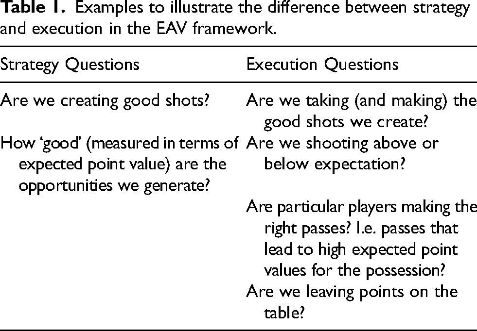
Examples to illustrate the difference between strategy and execution in the EAV framework.
Methodology
In our proposed method, we simplify the development of the traditional EPV metric to the most fundamental decisions that an NBA basketball player makes on the offensive end of the court: whether to pass or shoot and, in the case of a pass, who to pass to. We introduce a new metric Expected Action Value (EAV) to capture the expected value of these potential actions during a possession. With EAV, we seek to address the following two questions at any point in time:
If the ballhandler shot right now, would that be considered a good (i.e. high EAV) shot? If the ballhandler passes to a teammate, would that give a better shot option? What is the EAV of the combined pass and shot?
With this goal in mind, we define EAV as follows.
The expected number of points to be scored by an offensive player
Unlike EPV, we have defined EAV as a function of both time and player, such that each offensive player has an EAV at every moment during a possession. The ballhandler’s EAV captures the action of them shooting, while each other offensive player’s EAV captures the action of them being passed the ball before shooting. By mapping each of the actions in our action space to each offensive player one-to-one, we can logically interpret EAV as being parameterized by player.
Given that we know where the ball is (and correspondingly who the ballhandler is), the expected points for player 
Evidently, the computation of EAV hinges on probability predictions, namely probabilities of pass completion and shot conversion. To estimate these probabilities, we develop shot difficulty and pass difficulty models as neural networks that take tracking data and game metadata as input, outputting a probability of success. These predictions are then leveraged to compute a series of EAV values for all time frames, for all offensive players during a possession. This paradigm is summarized in Figure 1.
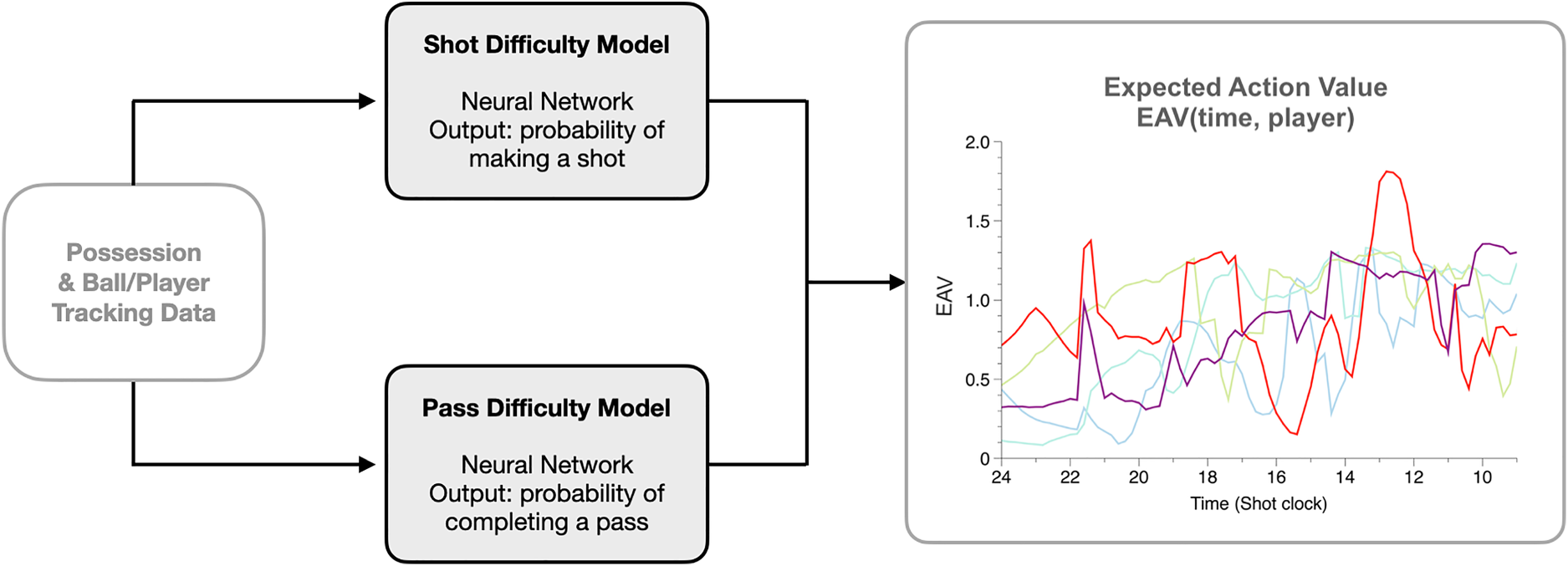
Expected Action Value (EAV) calculation diagram. EAV for each offensive player at each time frame is calculated by passing tracking data through two difficulty models: shot difficulty and pass difficulty. The outputs of these two models are combined to estimate EAV. EAV evolution for each player throughout a possession can then be visualized as shown on the right; each color represents a different offensive player.
This approach diverges from the EPV traditional method, though both seek to calculate a similar expectation. The development of EPV is centered around the modeling of future possession trajectories over a long time horizon, which is not considered in our EAV computation. Our intention is to provide an instantaneous evaluation that can be associated with individual actions, agnostic to prior and future events. In the context of our particular decision-making metric, we believe this to be a valid simplification, as the first-order immediate actions largely mirror the decisions that players are making. Furthermore, this reduces the uncertainty from the vast space of all future possession paths to just the potential outcomes of immediate passes and shots. It also eliminates the need in our approach to model future player movement, another source of uncertainty. Finally, EPV is constructed with an ensemble of parameterized stochastic models, whereas we experiment with a deep learning architecture for our difficulty prediction task. The details of the difficulty models are discussed next.
Difficulty models
We frame the probability prediction of these models as a supervised learning task. In contrast to previously developed shot difficulty models, we utilize a deep learning approach in an effort to maximize expressive power for accuracy (Bozak and Aybek, 2020). To that end, we develop two neural networks: one for predicting pass completion probability and one for predicting shot conversion probability. For the sake of simplicity and computational feasibility, we restrict the sizes of both the pass and shot difficulty model to be small in architecture. Each network is designed to take as input a feature vector characterizing the pass or shot, outputting a probability prediction.
Model features
By design, our feature vectors were generated only from the game and tracking metadata. We curated a set of explanatory variables that could be easily derived from the tracking data for characterizing both passes and shots. The main features that can be extracted from the tracking data are geometric components that correspond to relative distances and angles between entities involved. For passes, the key distances include passer to target, passer to basket, and target to basket, while the angle formed by the line segments passer-basket-target is a key angle feature. For shots, shooter to basket distance is the primary distance feature used, with the ‘offset’ of the shooter captured as the angle formed by the line segments shooter-basket-midcourt.
We also leverage the defender location data to incorporate defensive configuration features, roughly characterizing how much defensive pressure there is on a pass or shot and how likely those defenders are to disrupt the play. For passes this includes the closest defender distance to the passer, closest defender distance to the target, and closest defender distance to the pass trajectory, which can be interpreted as the most ‘obstructive’ defender relative to the pass. For shots this includes the closest defender to the shooter, the angle of that defender with respect to the shooter and basket, and the number of close defenders.
A visual depiction of these key geometric features for passes and shots is shown in Figure 2.
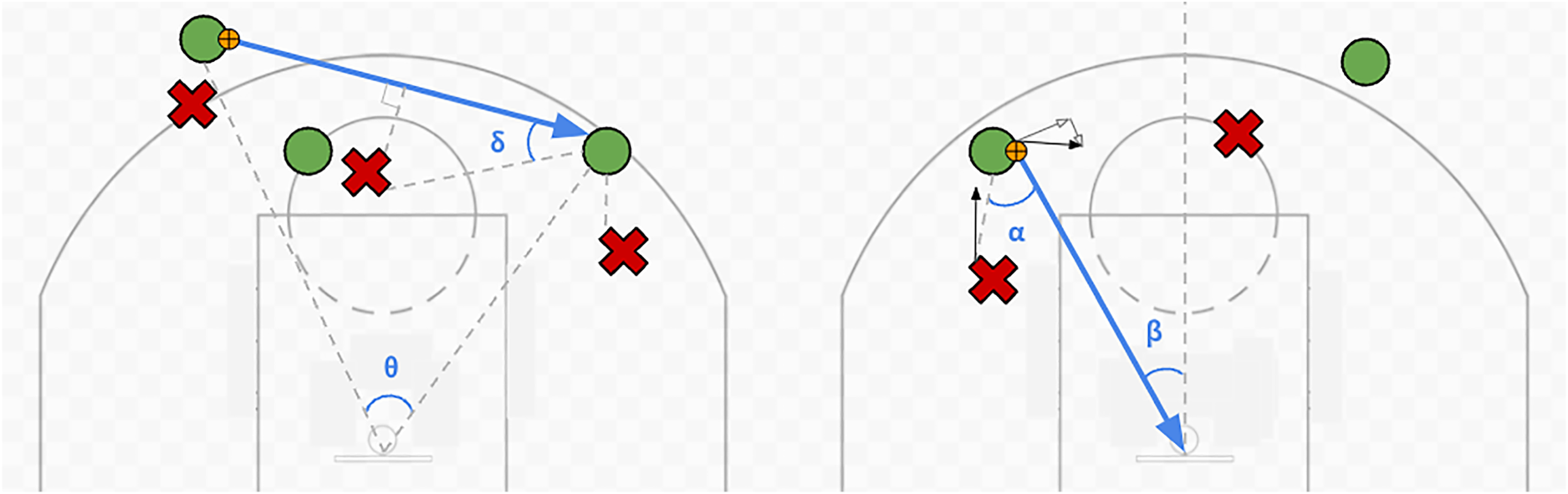
(Left) Diagram of geometric pass features. Blue arrow indicates the trajectory of a hypothetical pass. Green O’s indicate attackers, red X’s indicate defenders. The middle defender is most ‘obstructive’ defender, with the smallest perpendicular distance to the trajectory of the pass. The angle of the pass with respect to the basket is denoted by
One aspect of shots that makes them more difficult to predict relative to passes is the effect of the players’ movements leading up to the shot. If the shooter suddenly decelerates before taking the shot, or if their velocity is very high while taking the shot, it becomes much more difficult to make that shot compared to the same shot if they were standing still. Similarly, if a defender is jumping very quickly at the shooter or is accelerating towards them as they shoot, their actions are much more disruptive than if they were standing still. To capture these effects, we also include relevant velocity and acceleration information in the shot model. We compute velocity and acceleration values through iteratively applying a Savitsky-Golay (SG) filter to smooth the raw positional data and differentiating with respect to time (Savitzky and Golay, 1964). The data is smoothed with an SG filter of window size 5 frames; fitting the resulting points with a generic cubic spline to allow for continuous differentiation yields instantaneous velocity values in the first derivative, and acceleration values in the second derivative.
Finally, we include a few features that are based on game context. For example, we include a binary feature for passes that flags whether or not the passer and target are both located in the backcourt. Passes that occur completely in the backcourt are usually undefended, and so should be considered outliers by the model. By incorporating this explicitly as a feature, we expect the trained model to easily differentiate those situations. We also encode the time remaining on the shot clock into our feature vectors, as it may have an effect on the offensive pressure to execute a shot or pass.
A comprehensive list of all features used can be found in the Appendix in Tables A1 and A2.
A noteworthy omission from our feature set for the difficulty models is player identity, meaning that we do not consider the player-specific shooting, passing, or defending ability. While this information would improve the models’ predictive power, we choose to prioritize simplicity in our framework to achieve maximum generalizability. Incorporating individual player identities or sub-groupings of players at different ‘skill’ levels is an interesting question for future work; however, for the purposes of this study, we found that player agnostic models are sufficient for first-order decision-making analysis.
Model architectures and training
A primary objective for our neural networks is fast forward-pass inference speed. Since these predictions will be made at each time frame for multiple players, it was imperative to limit the depth and size of the network as much as possible.
Our pass difficulty model consists of one fully-connected hidden layer with 128 units, each activated with a ReLU function. Our shot difficulty model required more complexity, using four fully-connected hidden layers with 512 units each, activated with a leaky ReLU (Xu et al., 2015). For both models, we include a dropout layer with dropout parameter 0.2 after each fully-connected layer as a form of regularization (Srivastava et al., 2014). Each model has an output layer that is fully-connected, using a sigmoid as a final activation to convert the output into a probability.
In training our pass difficulty model, we needed to account for the heavy imbalance in our training dataset towards completed passes (i.e. most passes in the NBA are completed). We addressed this by weighting the loss incurred by each training example with the inverse frequency of the class, such that misclassifying an incompleted pass would result in a much larger loss than that of a completed pass. In particular, letting 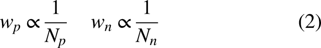
Expected action value
Equipped with a framework for characterizing shot difficulty and pass difficulty as probabilities of success, the computation of Expected Action Value becomes a simple evaluation of Equation (1). Recall that the goal of Expected Action Value as a metric is to capture the hypothetical scenarios created by the ballhandler deciding to either shoot or pass to one of their teammates to shoot, quantifying how many points the team can expect from any one those decisions. Calculating this expectation is nothing more than weighting the probability of success with the corresponding point value. Leveraging both the shot and pass difficulty models, we characterize how likely it would be to first get the ball to each offensive player, then subsequently how likely it would be for them to score. We make the trivial assumption that the probability of the ballhandler completing a pass to themselves is 1.
While we receive tracking data at a 25 Hz frame rate, we only run EAV calculations at a 5 Hz frame rate for computational efficiency, which we found empirically to be qualitatively equivalent. For each frame, we compute EAV values for all 5 offensive players, resulting in
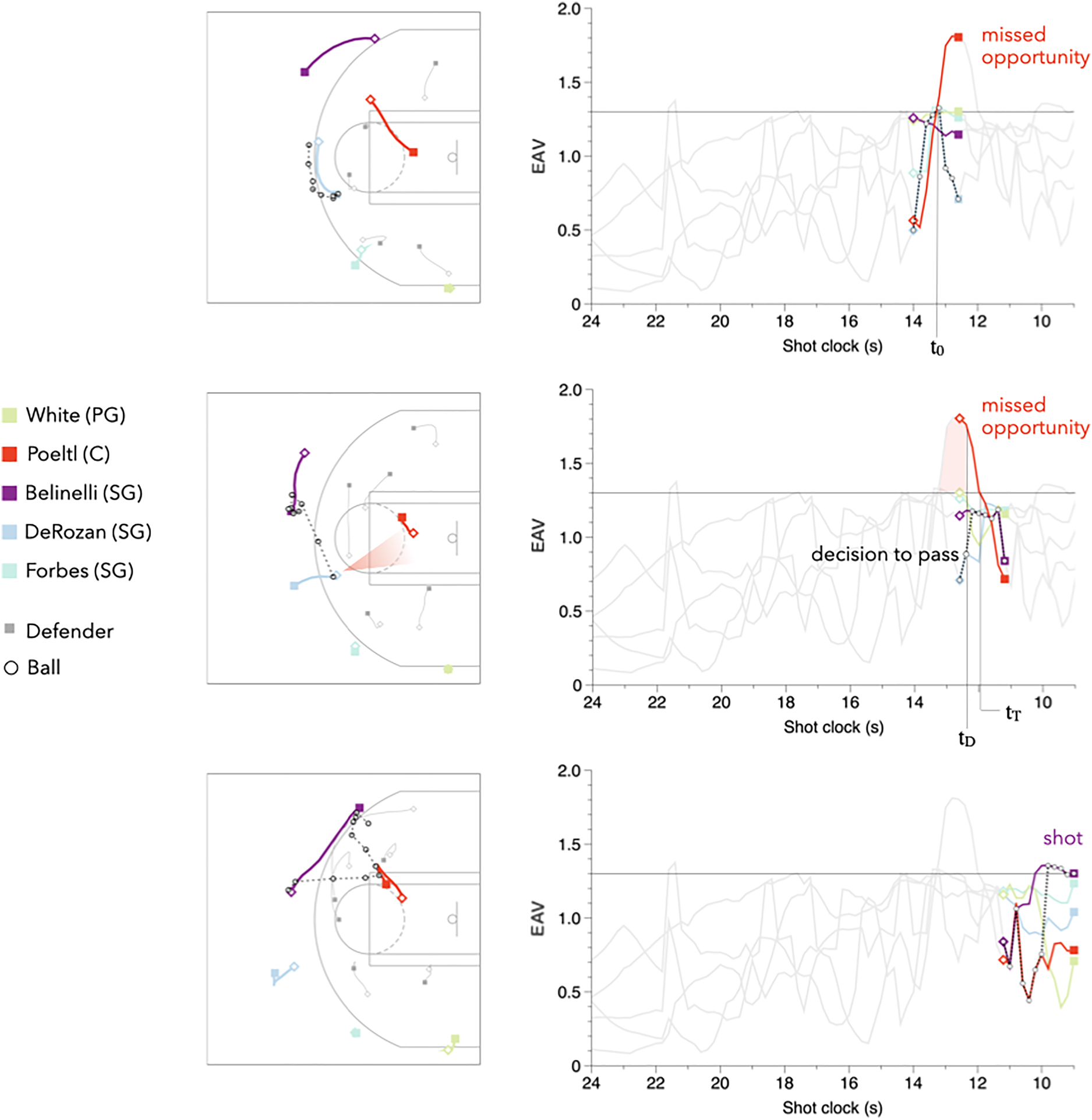
Example of a missed pass opportunity EAV visualization. Evolution of possession is read from top to bottom. (Left) Diagrams depicting players and ball positions, with player movements shown as lines from open diamonds to filled squares. (Right) Corresponding EAV values for each offensive player throughout the possession; the ball (and hence the ballhandler) is depicted by an open circle and the ballhandler EAV by the dotted black line. A missed opportunity is depicted by the spike in the red curve (Poeltl) who does not receive the ball in that duration despite having the largest EAV. (Denver Nuggets @ San Antonio Spurs; December 26, 2018; possession starts with 9:44 remaining in the 4th quarter, Denver Nuggets leading 80-79).
Missed opportunities
EAV values give us the power to reason counterfactually about hypothetical passes that could have been made and hypothetical shots that could have been taken. Quantifying these instances allows us to compare what actually happened versus what could have happened, uncovering insights about how effective players and teams are at capitalizing on opportunities as they arise.
In our work, we categorize opportunities as being either ‘shot’ or ‘pass’ opportunities, which are both dependent on EAV values exceeding a certain threshold. Intuitively, we can identify opportunities as instances of high EAV where an action could be taken to attain a high number of expected points from the possession.
An instance in which a ballhandler’s EAV exceeds a given threshold for one second or longer. The opportunity is ‘missed’ if the ballhandler does not shoot in that duration.
(Pass opportunity)
An instance in which a non-ballhandler’s EAV exceeds the threshold for one second or longer, and has the highest EAV out of all offensive players in that duration. The opportunity is ‘missed’ if the ballhandler does not pass the ball to this player in that interval.
Letting 
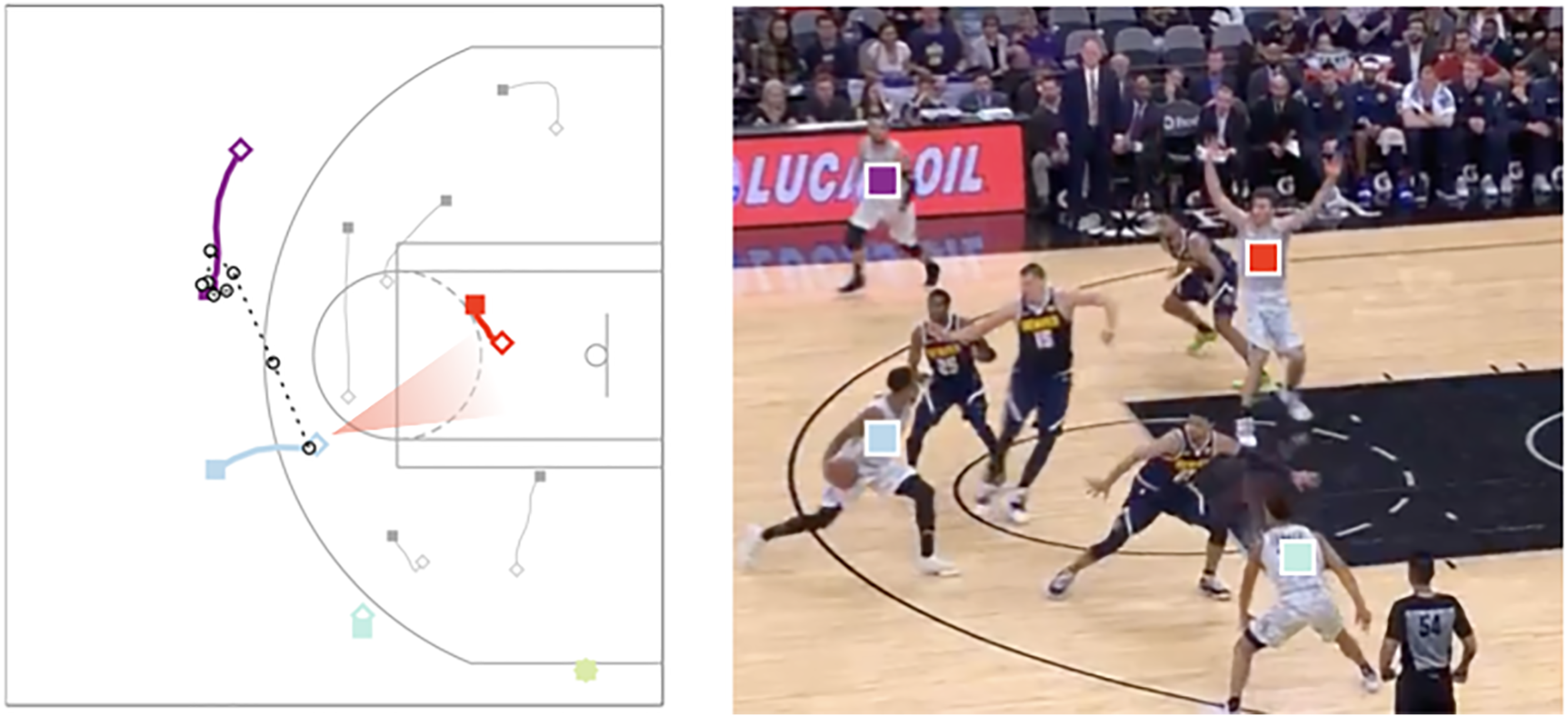
Broadcast view of the missed opportunity example shown in Figure 3. The red square indicates the missed pass opportunity identified by the algorithm.
With a large corpus of opportunities and classifications of whether they were missed or not, we can now evaluate, on a player level, who is good at identifying and taking advantage of these opportunities. We can also evaluate on a team level which teams are good at creating opportunities, indicative of good strategy and game plan, and which teams are good at taking advantage of their opportunities, indicative of efficiency and execution ability. To this end, we define a player’s or team’s missed opportunity rate (MOR) as the fraction of total opportunities that a player or team misses:
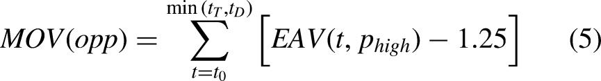
Finally, we compare the maximum EAV of the missed opportunity with the resulting EAV of the ballhandler’s actual decision, defining the difference between the two values to be the missed opportunity delta (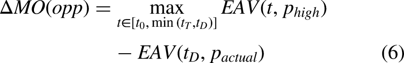
Leveraging EAV to identify inefficiencies through missed opportunities may prove to be valuable for NBA teams as they look for every competitive edge, and is the primary application of our EAV development thus far. In our discussion section, we expand on the analysis around decision-making, strategy, and execution for both teams and individual players through an opportunities lens.
Results
Model performance
Our training and test data consist of all 786,208 passes from the 2018-2019 NBA season and all 1.4 million shots from 2013-2019, collected by Second Spectrum. We trained each model for 10 epochs using a stochastic gradient descent (SGD) optimization algorithm with a binary cross-entropy objective function, which was sufficient for convergence (Ruder, 2016).
Our pass difficulty model achieved a 0.885 ROC-AUC accuracy score, while our shot difficulty model achieved a 0.620 ROC-AUC accuracy score. Due to the inherent variability in shot conversion, in which multiple shot samples with identical input features may result in both makes and misses, there is an upper-bound to the overall predictability. We believe our performance is close to this upper bound; the fact that the average field goal percentage in the NBA is approximately 45%, suggests that the maximum predictability for any such model will not be significantly greater than 0.55.
The existing work in literature seeking to predict shot conversion probabilities supports this empirically, all having reported accuracy metrics comparable to our shot difficulty model. Chang et al. (2014) report a maximum predictability of 0.633 using a similarly defined ‘shot quality model’; Harmon et al. (2021) utilize a CNN (convolutional neural network) based approach to achieve an accuracy of 0.615; Aitcheson-Huehn et al. (2024) leverage visuomotor control data in a decision tree classification approach to achieve an accuracy of 0.580. We use these comparisons as validation that the performance of our difficulty models is inline with other studies in the literature.
EAV evaluation
We ran EAV computations for each NBA team’s first 400 possessions in January 2019 while simultaneously keeping track of defined opportunities. We found 400 possessions to be a sufficient sample size for average player and team opportunity metrics to converge. Using a non-hardware accelerated Jupyter virtual machine, running EAV computations for a total of 12,000 possessions took approximately 20 hours, at roughly 10 minutes per 100 possessions (Akidau et al., 2015). As the average duration of an NBA possession is approximately 14 seconds, our EAV computations run 2.3x faster than real-time, suggesting that this framework can be used in a low latency live environment.
To test the reliability of our EAV metric, we evaluate its predictive ability against actual game scores. We use our framework to compute the expected points for each possession’s final shot and sum up those values over the course of each game for each team. For shots where a shooting foul occurred, we only include those in which the basket was made. We then compare these point total predictions to the actual points scored by each team, excluding converted free-throws (Basketball-Reference, 2019). This comparison is depicted in the left frame of Figure 5, where each data point indicates the team’s actual score on the x-axis and the corresponding aggregated EAV prediction on the y-axis. Since we do not use this data to inform our model development, we perform it as a single evaluation in place of cross-validation.
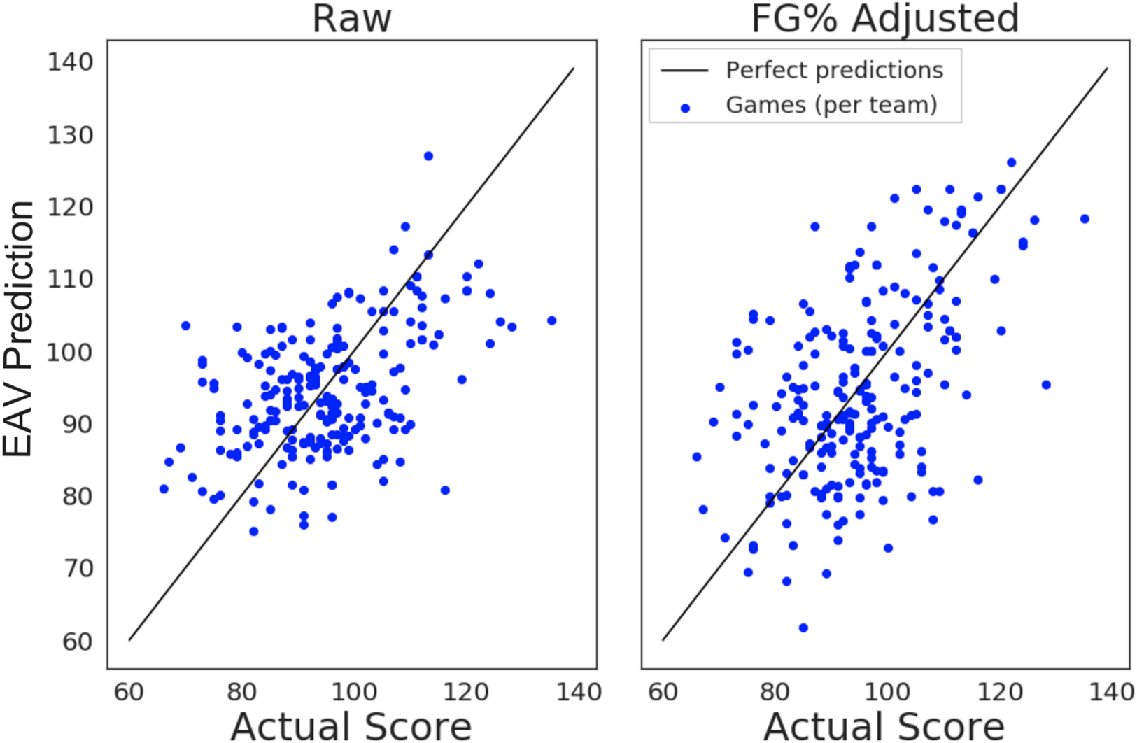
Evaluation of EAV accuracy by comparing EAV predicted game scores and actual game scores. (Left) Raw EAV predictions. (Right) Adjusted EAV predictions based on team field goal percentage.
A perfect EAV prediction for a team in a game would give us a data point that lies on the black line, indicating that the EAV predicted point total exactly matches the actual point total. Thus, a perfect prediction framework would generate points that all lie along this line, such that the Pearson correlation coefficient 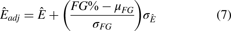
Distribution comparison of EAV predictions to actual scores.
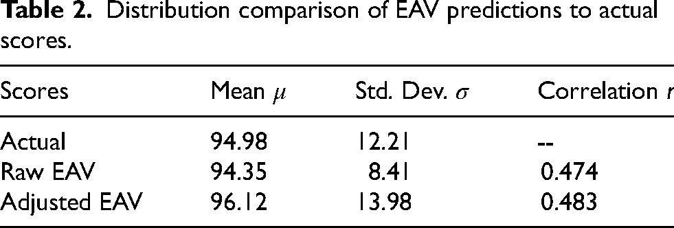
This gives us a rough interpretation of the predictive power of EAV. In general, EAV captures the difficulty of shots decently well. However, the high discrepancy in shooting ability among NBA teams is reflected in the comparison of these two plots, which our EAV by itself does not yet encapsulate. This is unsurprising given that we did not include player identities or any form of player specific shooting ability metrics in our development of EAV; including shooting ability in the training and inference is possible, but introduces a level of complexity that becomes computationally expensive and difficult to maintain. Yet we see here that even incorporating minimal shooting ability information as a post-processing correction improves EAV accuracy.
Discussion
We found that there is significant value to using a machine-learned process as we do in our calculation of EAV. First, we don’t have to incorporate basketball-specific information into our model. Instead of manually encoding domain specific actions such as ‘ball denial’ from the defender, or ‘contested jump shot’, we simply construct a rich enough feature set from the raw tracking data to let the model learn these relationships. This minimizes the amount of biases about the game of basketball that we – the model developers – inject into the model, which results in a more objective system as a whole. The other substantial benefit to using a machine learning approach for computing EAV is its ability to generalize to the vastly different styles of passes and shots in offensive basketball. Typical heuristics-based models require many conditional paths with manually set thresholds to cover ‘types’ of passes and shots that can occur. This is not scalable for a domain with a large search space.
To illustrate these points concretely, consider the example missed opportunity from Figures 3 and 4. Our model has no understanding of what a ‘slip screen’ or a ‘cut to basket’ is, which are terms that one could use to describe what is happening in this possession. These scenarios are often hard to classify even to the human eye, so we choose to develop our model as semantically detached, instead using features like distance to basket and nearby defenders for a simpler objective characterization of the play. Furthermore, this exact play does not appear in our training data, nor do we teach the model anything specific about this particular possession. We did not hard-code concepts such as ‘being close to the basket is high value’ or ‘an open passing lane is good’, concepts which would be required to capture this scenario properly in a heuristics-based approach. Instead, the machine learned model has generalized its mapping of feature set to outcome prediction without basketball semantics level information, and is able to accurately determine the EAV to be high based on raw features alone.
Evaluating decision-making
Individual decision-making
To understand how we can leverage our opportunity framework to quantify decision-making, we first look at opportunities on a per-player basis. In particular, we calculate each player’s average missed opportunity rates and average missed opportunity values, differentiating between shot and pass opportunities. Figure 6 depicts a player cloud showing where players fall on a pass opportunities plane. The plane is defined first by the number of pass opportunities that player has per second on the offensive end for their team, a proxy measurement for how ball dominant they are. The second dimension is their adjusted missed opportunity rate. For the sake of analysis and comparison, we adjust each player’s MOR to account for general shooting ability, corrected according to free throw percentage then normalized to a 0-1 scale.
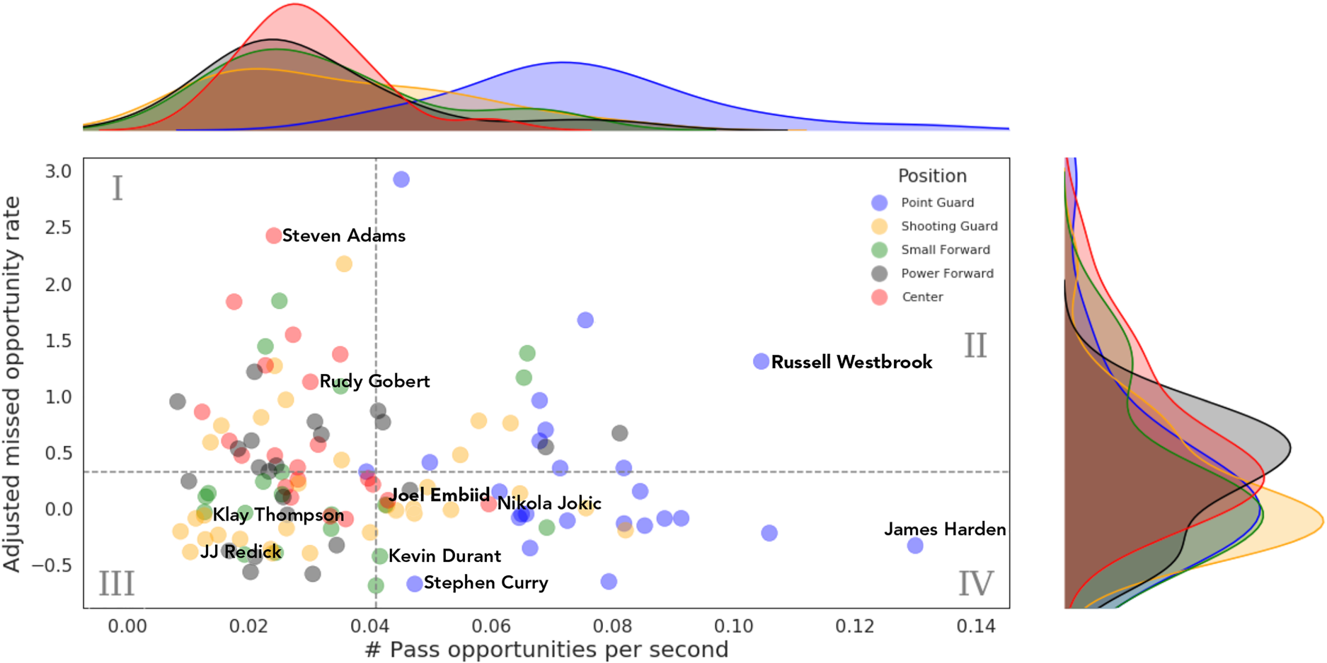
Player cloud of pass opportunities per second versus adjusted missed pass opportunity rate (pass
The plot is separated into four quadrants (by axes medians), each of which can be characterized in basketball terms and related to decision-making. Better than median missed pass opportunity rates are below the horizontal dashed line in the bottom two quadrants, a general indicator of ‘better’ decision-making. Unsurprisingly, this area is comprised of mostly guards, whose decision-making generally plays a large role in their success. The area is further split by the vertical line, separating ball-dominant and off-ball players. The ball-dominant players (quadrant IV) have a heavy concentration of skilled point guards such as Stephen Curry and James Harden, while the off-ball players in this area (quadrant III) consist of primarily catch-and-shoot shooting guards, including two of the most prolific three-point shooters in NBA history, JJ Redick and Klay Thompson. A player like Kevin Durant, who often played off-ball during this time in his career on the Warriors but was still extremely efficient as a scorer, falls in the middle. Two positional exceptions are centers Joel Embiid and Nikola Jokic: skilled, ball-dominant bigs who can facilitate just as effectively as they can score. This plot captures their uniqueness in play-making ability relative to others in their position group.
If we look at the upper two quadrants, we see that the upper left (quadrant I) consists predominantly of bigs. For the big men, the high missed pass opportunity rate is reasonable, as once they have the ball in their hands it is usually not their job to facilitate and pass. Players in this quadrant like Steven Adams and Rudy Gobert are used in lineups not as play-makers, but rather for defending and rebounding prowess.
The group that stands to gain the most via adjusting their strategy or ‘court-sense’ when it comes to decision-making is in the upper right quadrant (quadrant II). These players not only have high missed opportunity rates, but also spend a lot of time during possessions with the ball in their hands, and thus are presented with pass opportunities more frequently. While the roles of these players are similar to those in quadrant IV, their inability to shoot effectively yet deciding still to do so, results in more missed pass opportunities. To make the most of these high-usage players, strategies should be adopted (either through individual player training or by modifying the team tactics) to lower their missed opportunity rate.
An interesting exception in this quadrant is Russell Westbrook, who was the focal point of the Oklahoma City Thunder’s offense at that time, ranking #10 in the league in usage percentage (30.9%). Westbrook was one of the league’s best players during this time period, averaging a triple-double with 23.1 points, 12.2 assists, and 11.2 rebounds per game. While our decision-making evaluation framework assumes a well-defined optimization target of maximizing team expected points per possession, the team’s optimization function was likely skewed by a secondary goal of getting Westbrook a triple-double. This is a perfectly reasonable objective and arguably aligns with the NBA goals of making the game exciting to fans. Interestingly, this difference in objective resulted in statistics that profiled Westbrook as an inefficient volume shooter, as that year he ranked #4 in the league in field goal attempts per game (20.2), while ranking #117 in effective field goal percentage (46.8%). However, it also resulted in Westbrook leading the league in assists per game (10.7) (Basketball-Reference, 2019). Evidently, this demonstrates that our – and indeed any decision-making evaluation framework – is (correctly) subject to differences in objective; and consequently decision-making evaluations and conclusions can not be made without considering all factors. In addition, it is clear from this example that raw statistics, such as assists and shots, are not rich enough to express a true evaluation of decision-making.
This motivates the most interesting way to analyze this player cloud from a decision-making standpoint. In reality, when evaluating player decision-making ability relative to others, we need to control for how ball-dominant the players are, which in turn dictates the frequency of opportunities that arise. Thus, we should be looking at any vertical slice in the plot to group players with similar levels of opportunities, only comparing that subset of missed opportunity rates to make judgements about relative decision-making ability.
Team decision-making
Next we repeat a similar opportunity analysis but on the team level, this time with shot opportunities instead of pass opportunities, shown in Figure 7. In the team context, our 2-D plane of shot opportunities and missed opportunity rates can be interpreted as strategy versus execution. One goal of an NBA offensive strategy is to generate high value shots on every possession. The number of high-quality shot opportunities a team can generate is one measure of the quality of their offensive strategy. However, the quality of their execution depends on how often they are actually able to capitalize on those shot opportunities.
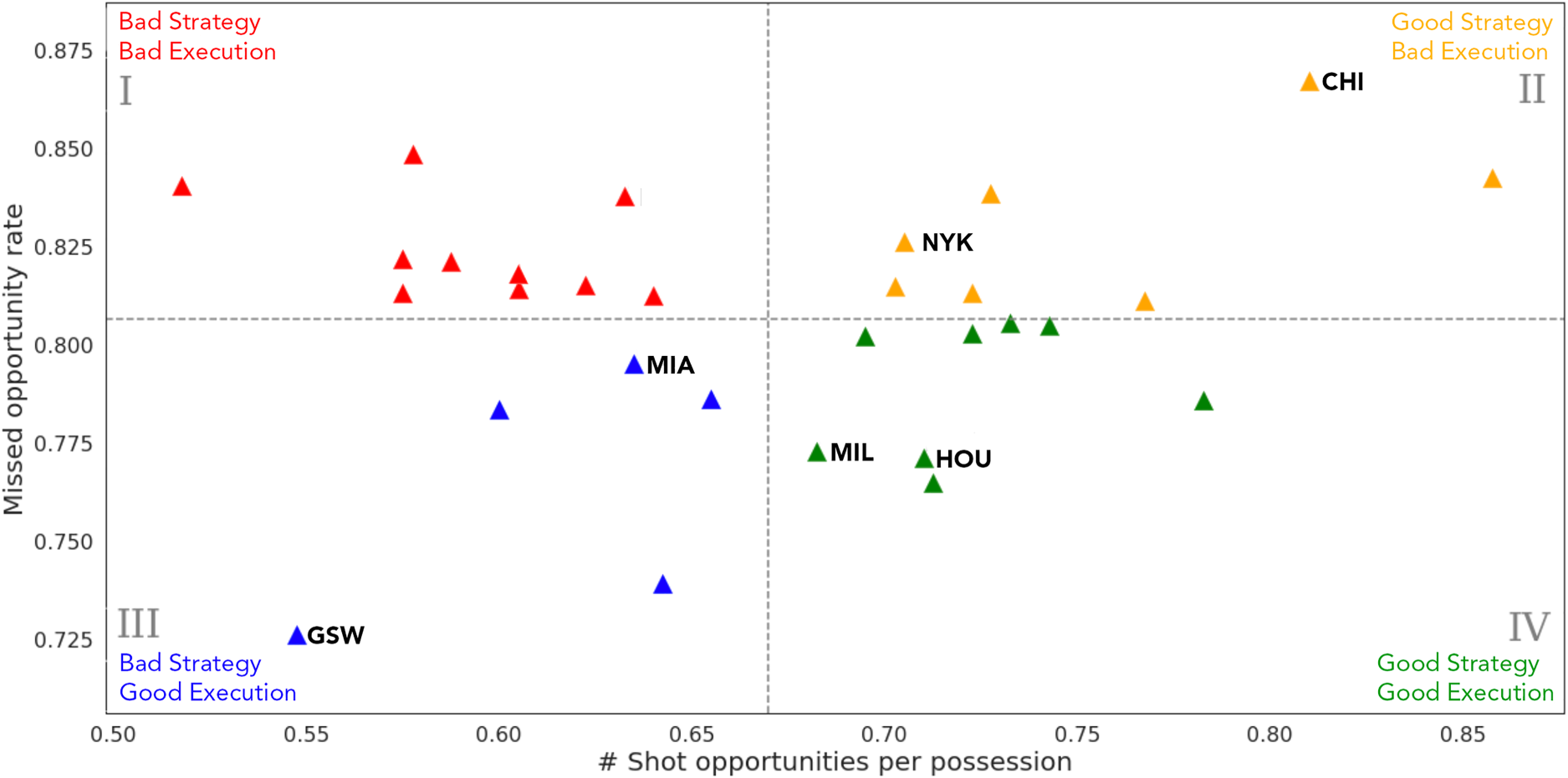
Team cloud for January 2019 showing the number of shot opportunities compared to missed shot opportunity rate. The number of opportunities increases with better strategy; missed opportunity rate increases with worse execution. High-performing teams are expected to be found in quadrant IV.
Again we break this plot into quadrants according to axes medians to identify where teams fall relative to the rest of the league. The best quadrant is the lower right (quadrant IV): good strategy and good execution. We see here a couple of high-powered offensive teams in 2019 such as the Houston Rockets, who ranked #2 in adjusted offensive rating (ORtg/A), and the Milwaukee Bucks (#4 in ORtg/A). On the other hand, we see teams that struggle offensively both with gameplan and execution in the upper left quadrant (quadrant I). This quadrant is generally characterized by less potent offenses, as the average ORtg/A of this group would rank #17 in the league.
The more interesting quadrants from an analytical perspective are the upper right (quadrant II) and the lower left (quadrant III). The teams in the upper right quadrant had weaker ORtg/A ratings in 2019, which can largely be explained by their high missed opportunity rates (i.e. inconsistent offensive execution). These teams include the Chicago Bulls (#29 in ORtg/A) and New York Knicks (#30 in ORtg/A). The difference between these teams and their counterparts in quadrant I is that these teams have well-developed strategies to generate good scoring opportunities; but they struggle on the execution side and are unable to capitalize on those generated opportunities.
The lack of consistent execution for teams in in quadrant II may be attributable to lack of experience in the NBA, as both of these teams were among the youngest in the league that year. Weighted by minutes played, the average age of the Knicks and Bulls were 23.3 and 24.1, the youngest and third youngest teams in the league, respectively. Given their sound opportunity generation scores, with additional experience we’d expect improved execution, which would result in a shift vertically downwards in the plot.
In quadrant III, we see a particular interesting outlier in the Golden State Warriors, who were dominant in the NBA during this period (#1 in ORtg/A). The plot suggests that their success was not necessarily due to their strategy or gameplan, but rather was primarily attributable to their historically great shooting ability and elite execution. For a team that did not look like there was much room for improvement, perhaps their performance could have been optimized further with the creation of more high quality shots, corresponding to a shift horizontally to the right in the plot. A weaker offensive team in this quadrant such as the Miami Heat (#26 in ORtg/A) stands to gain even more with the same philosophy (Basketball-Reference, 2019). These teams are likely to see more gains from prioritizing improvement in offensive strategy and gameplan rather than from training for shooting ability.
Points for the taking
Through identifying opportunities and analyzing how players and teams react to those opportunities, we have shown that using the expectation based metric EAV can provide a framework for quantitatively evaluating decision-making, team strategy, and execution on the offensive end of the court. Because this metric relies on expectation and not on outcome, it is not necessarily intuitive to those without a statistics background. In this final section we translate the analytical framework into the language of ‘points left on the table’ and consequently, wins and losses, explicitly highlighting potential improvement in performance.
Looking at the missed opportunities on a game-by-game basis, we pose the question: if a team had a 0% missed opportunity rate (i.e. if they had capitalized on every opportunity in the game), how many additional points could they have scored? We answer this by summing up all the missed opportunity delta values, as defined in Equation (6), throughout the game (again, omitting free throws). This effectively captures the difference between what the team actually did and what they hypothetically could have achieved using the same strategy, with better execution.
In Figure 8, we show the distribution of actual game scores as well as the distribution of potential points scored with optimal EAV decision-making. The difference in means between these two distributions is 30.4 points, an average improvement margin of 33%. With roughly 11 points being the average margin of victory in the NBA, capitalizing on just 37% of missed opportunities would be enough to flip a loss to a win, on average (Basketball-Reference, 2019). It is important to note that not all missed opportunities should be characterized as ‘mistakes.’ There are many reasons why, at any point in the game, a team or a coach may opt for a decision that does not produce the highest expected value: tactical game clock management, the element of surprise, the emotional state of the player, team or individual preferences, may all tip the scale in favor of a mathematically sub-optimal decision. However, given the large number of potential points left behind, our analysis hints that some of these are worth collecting.
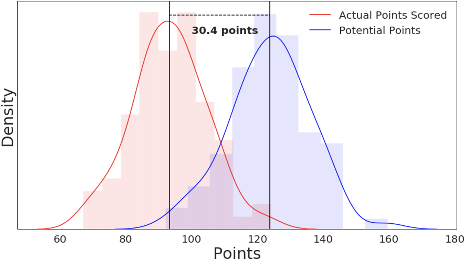
Distribution of actual points scored (red) compared to potential points per game (blue) which, on average, would have been scored if teams fully capitalized on all opportunities.
These results highlight the utility of EAV as a means for extracting insights about inefficiencies. This EAV lens suggests that teams have the potential to score many more points in a game (and thus win more games), as well as provides actionable insights as to why that is not happening currently, and what the coaching staff may need to do to address it.
Applicability
One of the strengths of our EAV approach and its simplification of search space and time horizon is the computational efficiency compared to the traditional EPV model. This reduction in computational complexity enables the EAV framework to be applied in a real-time setting for NBA teams and analysts. Cervone et al. (2016) acknowledge this as a limitation to their EPV method, specifically that the computational requirements for forward inference may serve as a barrier for adoption beyond academic circles.
While the authors note that a priority was maintaining computational tractability through using a multi-resolution approach, the forward inference procedure of repeated sampling from parameterized models remains a slower and more computationally expensive process compared to an optimized forward pass through a neural network. Each computation of EPV consists of alternating samples from the player movement model and the ball action model to construct future possession events, followed by event outcome sampling with a weighted point value. Each of these unique samples is a series of matrix computations from its respective model, comparable from a complexity standpoint to one forward pass through our fixed size difficulty models. Because samples can be drawn arbitrarily into the future (capped at 24 seconds for the maximum duration of a possession), the number of operations for a single frame can be quite high. For a single computation of EPV, letting
This allows our neural network based EAV framework to be applicable in real-time settings where expected point evaluations can be made at low latency with respect to live play. As empirically demonstrated in Section ‘EAV Evaluation’, our framework indeed runs faster than real-time with suitable resources, and thus may be of use in live environments. To enable this ability, our method sacrifices the complexity of incorporating the EPV past and future possession context, a trade-off that potentially reduces the semantic accuracy of our metric in comparison. We make this trade-off for the sake of evaluating immediate individual decision-making as opposed to decision-making throughout a possession, while enhancing the real-time applicability of such a metric.
Improving the framework
While we have shown this implementation of EAV to be a potentially powerful tool for decision-making evaluation in basketball, there are ways to improve our algorithm.
Including player identities in the EAV model itself rather than normalizing results by free throw percentages is a promising extension for model accuracy. Since EAV includes a measure of shooter success likelihood, encoding various facets of the players’ shooting ability would certainly provide a richer feature set. Analogously, encoding close defensive players’ defending ability into our features would also provide a more accurate depiction of the game situation we are analyzing. In addition to making the model more heavyweight with these additional features, including this information would require maintaining a large set of constantly changing player metadata within the system. In this iteration of EAV, we choose to use a much lighter-weight framework for the sake of simplicity; and indeed the feature set we included was sufficient to differentiate performance at the level of granularity required for our objectives. However, with increased computing power, the model could be tuned to individual athletes.
Another simplification we choose to make is restricting the action space to just ‘pass’ and ‘shoot’. In reality, offensive decision-marking extends far beyond these simple actions: off-ball cutting, driving to the basket, drawing fouls, and general spacing on the court. The relationship between these actions and expected points scored is much more complex than passing and shooting, which is why we choose not to model those aspects of the game in our EAV computation. Despite limiting the action space in our analysis, we believe the model contains sufficient complexity to characterize the game in the pursuit of quantifying decision-making.
Conclusion
Motivated by the task of evaluating NBA players’ decision-making abilities, we have built a foundation for leveraging expectation to assess the value of hypothetical player actions. We used novel deep learning techniques to develop models that accurately quantify the difficulty of passes and shots, and demonstrate that these neural network approaches are comparable in performance to existing models. Through a simple integration of these models, we constructed an Expected Action Value metric, capturing the expected points a player will contribute if the decision is made to pass the ball to them. This highlights an important aspect of decision-making analysis that lies at the core of our analysis: quantifying hypotheticals and counterfactuals. The question ‘what if’ lies at the heart of every decision. By explicitly enumerating possible actions for a ballhandler in the form of passing to a particular player or shooting the ball, then explicitly quantifying the value of each of those actions, we build an evaluation framework that mirrors the player’s perspective.
Using this framework, we unlock a multitude of tools and insights into athlete decision-making and team efficiency. In particular, EAV allows us to identify opportunities in possessions where on expectation, a certain action would result in a high number of points. These opportunities serve as unique evaluation points in the game where one can zoom in and begin to quantify the quality of player decisions. Given that the objective is to maximize expected points in each possession, we performed an in-depth analysis of opportunities, seeking to understand how often those opportunities are missed and relating that back to decision-making. We found that indeed there is a surprising amount of room for improvement when it comes to capitalizing on these opportunities.
We then quantified this improvement by showing that teams were leaving a large number of ‘points on the table’, often to the point where collecting these points could change the outcome of the game. This illustrates the value that EAV and opportunities analysis can bring to the game of basketball, and hints at its potential in the evaluation of player and team performance.
As it stands, decision-making analysis is still very challenging to do objectively, and there is sparse research in this space. Our work offers a new perspective through expectation to evaluate cognitive ability of athletes via tracking data.
Footnotes
Acknowledgements
The authors gratefully acknowledge Google Cloud and in particular Eric Schmidt and Ramzi BenSaid for their technical guidance and support, and Felice Frankel and Christina Habib for assisting in the development of figures.
Funding
The authors received no financial support for the research, authorship, and/or publication of this article.
Declaration of conflicting interests
The authors declared no potential conflicts of interest with respect to the research, authorship, and/or publication of this article.
Appendix
Full list of shot features.
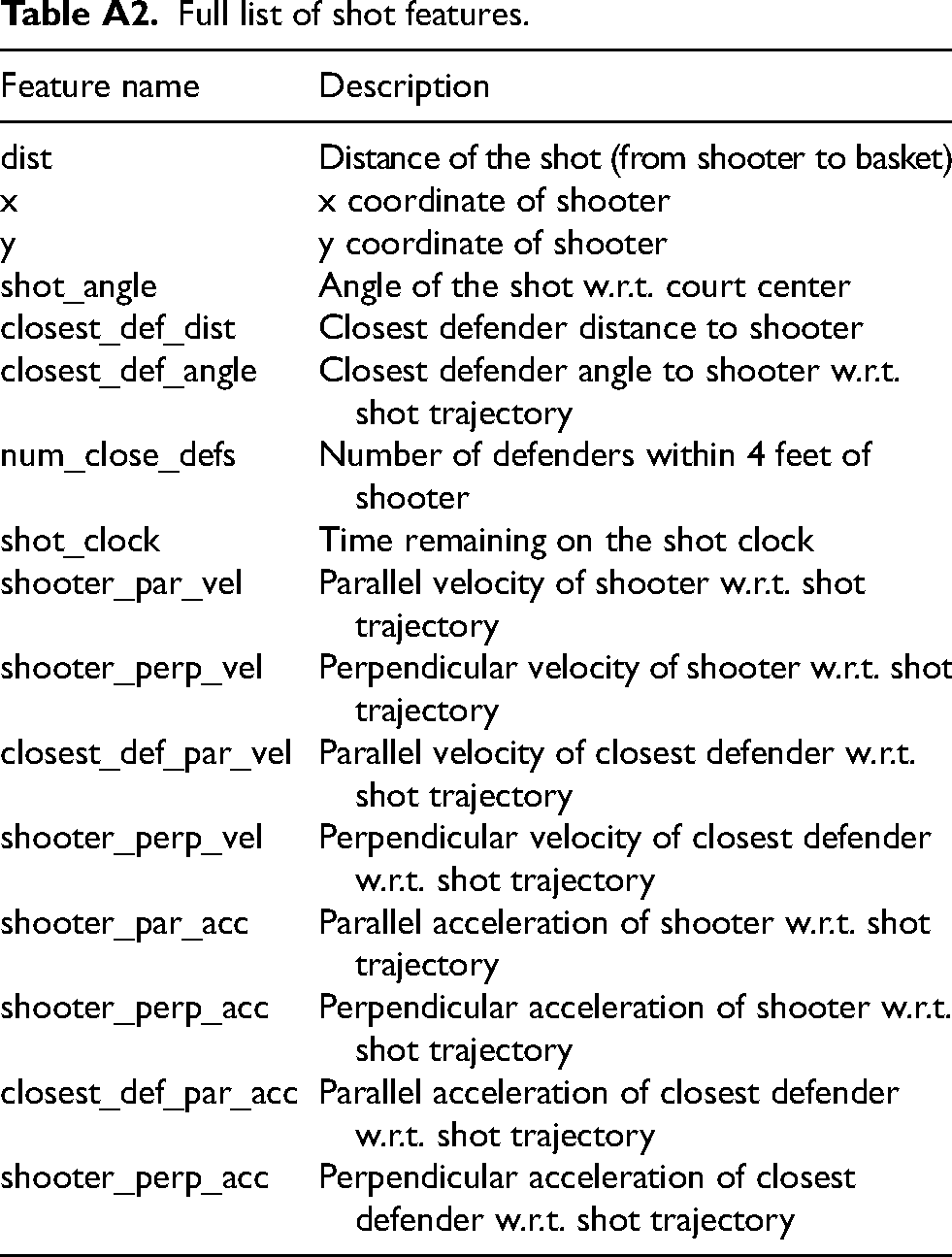
| Feature name | Description |
|---|---|
| dist | Distance of the shot (from shooter to basket) |
| x | x coordinate of shooter |
| y | y coordinate of shooter |
| shot_angle | Angle of the shot w.r.t. court center |
| closest_def_dist | Closest defender distance to shooter |
| closest_def_angle | Closest defender angle to shooter w.r.t. shot trajectory |
| num_close_defs | Number of defenders within 4 feet of shooter |
| shot_clock | Time remaining on the shot clock |
| shooter_par_vel | Parallel velocity of shooter w.r.t. shot trajectory |
| shooter_perp_vel | Perpendicular velocity of shooter w.r.t. shot trajectory |
| closest_def_par_vel | Parallel velocity of closest defender w.r.t. shot trajectory |
| shooter_perp_vel | Perpendicular velocity of closest defender w.r.t. shot trajectory |
| shooter_par_acc | Parallel acceleration of shooter w.r.t. shot trajectory |
| shooter_perp_acc | Perpendicular acceleration of shooter w.r.t. shot trajectory |
| closest_def_par_acc | Parallel acceleration of closest defender w.r.t. shot trajectory |
| shooter_perp_acc | Perpendicular acceleration of closest defender w.r.t. shot trajectory |