Sage Journals: Discover world-class research

Abstract

Evaluation of player value in sport can be measured in several ways. These measures, when captured over an entire career, provide insights concerning player contributions. Professional sports teams select young talent through a draft process with the goal of acquiring a player that will provide maximum value, but these expectations diminish as the pool of players grows smaller. In this paper, we develop valuation measures for draft picks in the National Hockey League (NHL) and analyze the value of each pick number with these measures. Specifically, we use different measures of player value to provide an expected value of that measure for each pick number in the draft. Our approach uses functional data analysis (FDA) to find a mean value curve from many observed functions in a nonparametric fashion. These functions are defined by each separate year of draft data. The resulting FDA model follows the assumption of monotonicity, ensuring that a smaller pick number always provides more expected value than any larger pick number. Based on a cross-validation approach, measuring value on annual salary provides the best predictive results. The proposed approach can be extended to sports in which an entry draft occurs and player career data are available.

Keywords

draft pick charts functional data analysis

Introduction

The National Hockey League (NHL) entry draft is an annual event held in the off-season to allow teams to acquire a prospect’s NHL rights. Draft-eligible prospects are typically ages 18 to 20 and come from Junior, College, or other pro leagues. The draft itself has been modified over the years, and consists of 224 picks over 7-rounds. With 32 teams in the NHL, this currently implies that each team receives 7 draft picks. The order of the draft is dependent on the standings from the previous season so the low-end teams get the earlier picks. More specifically, a draft lottery occurs prior to the draft, where the logistics of the lottery have changed over the years. In 2023, two draws were made to determine the top two draft positions from the 16 teams having the weakest records in the previous season. The remaining 14 draft positions were set according to team record. Under this lottery system, the worst finishing team from the previous season had a 25.5%, 18.8% and 55.7% chance of finishing first, second and third in the lottery, respectively. This is an attempt to promote parity in the NHL with an addition of randomness. The picks can also be traded amongst teams during, or in the years leading up to a specific draft.

The entry draft is a crucial moment on the NHL calendar as it is the opportunity to build for the future, with the goal of obtaining as much value through these picks as possible. As is the case with any sport, high draft picks (i.e. those chosen early in the draft) have a chance of becoming a “bust” or on the contrary, late draft picks have a chance of being a “steal”. Patrick Stefan was drafted 1st-overall in 1999 by the Atlanta Thrashers, which has been referred to as one of the worst draft picks in the history of the NHL (Bell, 2022). Stefan ended his career with 455 games-played and 188 points, an extremely disappointing career compared to most 1st-overall picks. By contrast, Pavel Datsyuk, who was drafted 171st-overall in 1998 by the Detroit Red Wings, finished his career with 953 games-played and 918 points, arguably one of the biggest steals in NHL draft history.

Chapter 12 of the book “Scorecasting” (Moskowitz and Wertheim, 2011) provides an engaging story involving the 1991 draft of the National Football League (NFL). In this draft, Mike McCoy of the Dallas Cowboys developed a chart that assigned perceived value to draft picks. The first draft pick was worth 3000 points, the second draft pick was worth 2600 points, and so on, in an exponentially decreasing order. With values assigned to draft picks, the Cowboys were able to trade picks to other teams, and accumulate value. Over the years, with better knowledge of the value of draft picks, the Cowboys had “fleeced” other teams, and set themselves up for a prolonged period of excellence that lasted for at least five years.

Since that time, many pick value charts have been created across professional sports. A sample of such contributions includes the National Basketball Association (Pelton, 2017), Major League Baseball (Cacchione, 2018), Major League Soccer (Swartz et al., 2013) and the National Football League (Massey and Thaler, 2013; Schuckers, 2011a).

In the NHL, there have been alternative constructions of pick value charts. Schuckers (2011b) used nonparametric regression on career games-played as a measure of player value. A review article on various issues associated with drafting in the National Hockey League was provided by Tingling (2017).

A major challenge in the construction of pick value charts is the determination of player value. Player value is an ambiguous term as it has different interpretations over the short term and the long term. Moreover, value is difficult to measure. For example, in hockey, goal scoring (a measure of excellence) is expected of forwards but not of defencemen. Teams may also hold different drafting objectives.

In this paper, functional data analysis (FDA) methods are used to construct pick value charts for the NHL. The rationale for FDA is that every draft season provides a range of player valuations, from the first draft pick to the last draft pick. Therefore, we argue that it is more sensible to regress the valuations on a yearly basis. That is, a year of valuations is considered a function, and FDA is concerned with the regression of functions rather than individual points. For an overview of applied FDA, see Ramsay and Silverman (2002). Another feature of the paper is that we assess pick value charts to give an indication of validity.

In Section DATA, we introduce the data where four metrics are proposed to assess player value. Importantly, we take into account the importance of considering performance metrics. The FDA model is described in Section Functional data analysis where its advantages are discussed with respect to pick value charts. The resultant FDA pick value charts are presented in Section Results where confidence intervals are provided. The inclusion of confidence intervals seems to be lacking from other contributions involving pick value charts. The quantification of uncertainty is important as teams need to make drafting decisions in light of uncertainty. We also validate the pick value charts via a cross-validation procedure which indicates that the metric based on salary percentile provides the best fit. We conclude with a short discussion in Section Discussion.

DATA

In this paper, we use three data sources. Sports Reference LLC (2022) data provides us with draft data from 1982-2016. This data are the full set of players that will be included in our analysis, even if players did not play in the NHL. The total number of players in this data is 8,613.

Vollman (2018) data provides us with player statistics from 1982–2006, including games-played (GP), goals (G), and assists (A), and advanced metrics such as point-share (PS). This data contains the players who played at least one game in the NHL. Of the drafted players from 1982–2006, we have player statistics for 2,803 players, including 72 players who were still active in the 2021–2022 season. Although more years of player statistics are available, we want to introduce player performance measures based on career contributions. Therefore, we truncate the draft data at 2006, allowing most players to complete their playing careers by 2022. We note that prior to the 1999–2000 season, there were only two points awarded for a single match. Subsequently, it was possible for three points to be awarded - if the match was tied at the end of regulation time, the loser received one point and the winner received two points. This rule change is incorporated in the PS statistic as calculated by Vollman (2018). Unfortunately, it means that point share is slightly higher after the rule change.

Lastly, Spotrac (2022) data provides contract information from 2001–2022 for players from the 2001–2016 drafts. This data includes the contract length, total value of the contract, and annual average value (AAV) of the contract. We calculate the percentile of each player’s AAV for all years under contract to normalize data in an effort to deal with inflation. In total, data was available for 1,144 players.

Data were cleaned as to match names across data sets. This included removing foreign letters, using full first names, and dealing with players with the same names to ensure consistency. A verification process was done to ensure all players were matched properly and no players were missed. We have ignored goaltenders from the data collection phase since various issues concerning goalies (e.g. performance, longevity) differ from positional players.

The NHL entry draft has evolved over the years as the number of teams in the league has increased. From 1982 to 1991 the draft consisted of 12-rounds, then fell to 9-rounds in 1995 and 7-rounds in 2005 which is now the present day amount. The current state of the NHL draft in 2022 involves 32 teams selecting for 7-rounds, for a total of 224 picks. There are rare cases of compensatory picks being awarded or picks being taken from teams due to violations of league rules, but those do not impact our analysis. To obtain a valuation of NHL draft picks, we truncate our data for past drafts to include only the first 224 picks. This applies to all drafts except 2006–2016 where less than 224 players were selected.

For our analysis, we only require a single explanatory variable, consistent with the proposed FDA framework. This variable will be the overall pick of the draft. Overall pick consists of the natural numbers $1, 2, \dots, n$ , where $n = 224$ is the total number of picks.

Measures of player value

This paper considers valuations of NHL draft picks using player statistics and salary information. A valuation will be obtained through four measures of player value. Measuring a player’s value is a difficult task as there are many ways to measure the quality of a career. A logical way is to use total games-played, as done in Schuckers (2011b), as this describes the longevity of a player.

Another way to view the problem is to use performance metrics as measures of player value. An advanced statistic, point-share, is what we will focus on. For this metric, a player’s value will be measured by both career average, and career total.

Although popular performance statistics (e.g. plus/minus) are measures of assessment, they are often confounded by other factors including the contribution of teammates. The use of salary data is another approach for player evaluation where we take the point of view that team executives (who determine salary) are knowledgeable about player value. This approach was utilized by Swartz et al. (2013) in the context of soccer.

Games-played ( $Y_{1}$ )

The first measure of player value, $Y_{1}$ , is games-played (GP). This has been the most widely used metric for player valuation as longevity is a valuable trait. Longevity is not only a valuable trait in a player, but it also describes the underlying value of the skill level of a player. There are only so many roster spots on NHL teams, and playing a high number of games means that a player warranted a roster spot, even when age became a diminishing factor on performance.

Using GP as a measure of player value does have drawbacks. One factor not taken into account is injuries. Injuries not only make players miss games but may also end players’ careers. For example, Mario Lemieux (drafted 1st overall in 1984), who is arguably one of the greatest players in NHL history only played 915 NHL games which ranks 492nd all-time. However, his points-per-game is second all-time only behind Wayne Gretzky, who played 1,487 games (24th all-time). Lemieux’s career was cut short by a variety of injuries, so using GP as a measure does not accurately represent the value that he provided during his career. Therefore, excellence over shorter durations is not captured by GP.

Another drawback is how teams and specifically general managers view the players they draft. There may be bias towards players drafted in the first round, especially in the top 5–10, because general managers do not want these picks to reflect poorly on their drafting ability. Also, these high-draft picks may be afforded more time to develop since they were seen to have great potential. Consequently, many high draft picks who become “busts” play more games than they would if they were a lower pick (Tingling, 2017).

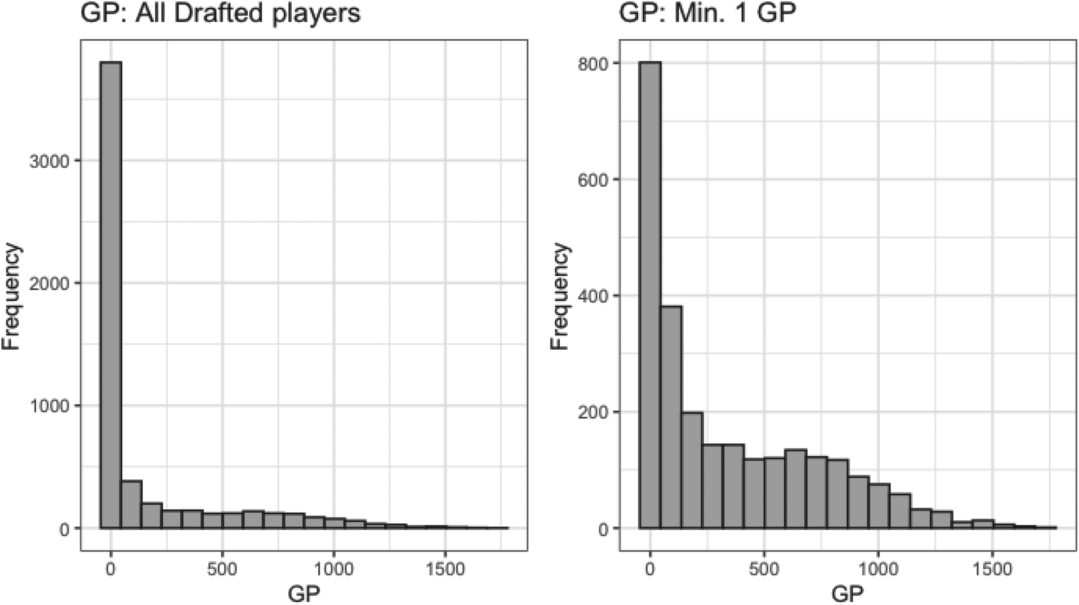
Figure 1 provides histograms of $Y_{1} = G P$ for all drafted players in our dataset. From the histogram on the left, we observe that the majority of drafted players never play a single game in the NHL. The histogram on the right provides the distribution of all players who played at least one game in the NHL, where we still observe that a large majority of players play very few games, and only a small number of players reach the 1000-game milestone.

Figure 1.

Histogram of games-played by all drafted players (left) and drafted players who played at least one NHL game (right).

Average point share ( $Y_{2}$ )

The second measure of player value, $Y_{2}$ , is average-point-share (APS). Point-share is an advanced statistic based on a similar baseball statistic called win-share created by Bill James. Win-share is calculated for each player based on their contribution (or lack thereof) to a win. NHL teams are awarded points for each game: two for a win, one for an overtime loss, and zero for a regulation loss. Therefore, APS is calculated for players so that the total APS for all players on a team closely matches the team’s point total for a season. For drafted players that did not play in the NHL, we set their APS value to the minimum APS in the dataset. The calculations for APS are detailed and will not be discussed fully in this paper. The full details are provided in Kubatko (2010). Perhaps contrary to intuition, Kubatko (2010) allows negative point shares with the explanation that “a player with negative point shares was so poor that he essentially took away points that his teammates had generated”.

A feature of APS is that it uses both offensive and defensive contributions, something that most statistics do not consider. Offensive contributions that are considered in APS include goal production relative to the player’s time on ice and relative to an average team. Defensive contributions that are considered in APS include goal prevention relative to the player’s time on ice and relative to an average team. Prior to 1998–1999 season, time on ice was unavailable and the point share statistic was based on games played. Since the goal of the NHL is to win games, evaluating a player’s contribution to wins is a reasonable measure of player value. However, measuring player value through team success may not fully capture a player’s individual value. In some cases there are high level players on low level teams that are undervalued in this metric. For example, during the 2007–08 season Marian Hossa was traded from the Atlanta Thrashers to the Pittsburgh Penguins. Hossa, who had 66 points in 72 games that season, went from the 28th ranked team to the 4th ranked team, increasing his PS even though his contribution was similar for both teams.

In addition, APS measures a player’s excellence, without examining their longevity. This will increase the value of players who had their career cut short by injury or other factors.

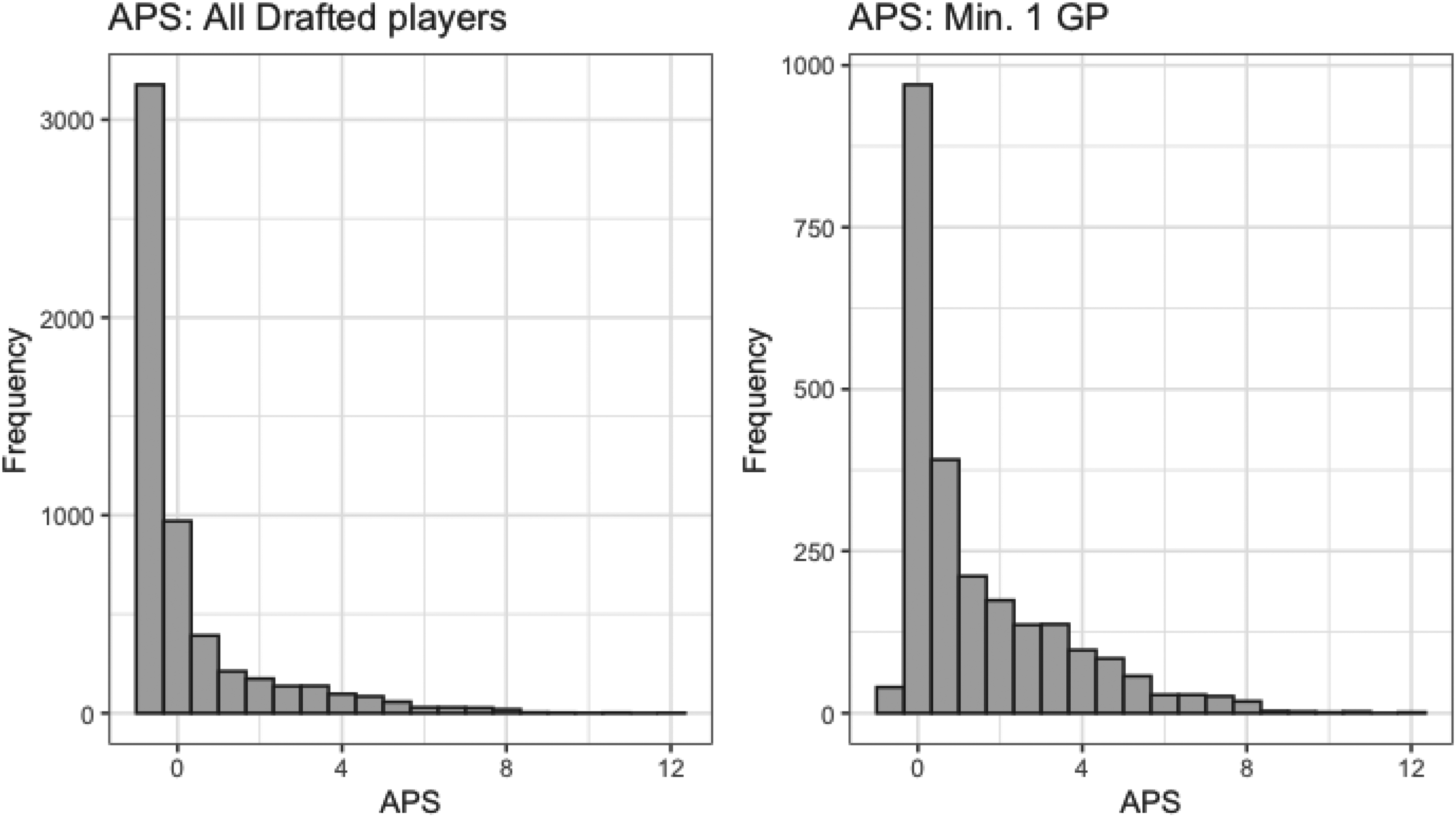
Figure 2 provides histograms of $Y_{2} = A P S = \frac{1}{S} \sum_{s} A P S_{s}$ , where $S$ is the total number of seasons a player played in the NHL, for all drafted players in our dataset and $A P S_{s}$ is the player’s APS in season $s$ . The histogram on the left includes every drafted player, so we see the majority of our data at the minimum value due to the large amount of drafted players who never made it to the NHL. On the right shows $Y_{2}$ for all players who played at least one game in the NHL, which still has the majority of players near zero. The exponential shape shows that elite talent is rare and most drafted players will have minimal contribution in comparison.

Figure 2.

Histogram of average-point-share by all drafted players (left) and drafted players who played at least one NHL game (right).

Total point share ( $Y_{3}$ )

The third measure of player value, $Y_{3}$ , is total-point-share (TPS). A description of APS has been provided in Section Average point share ( $Y_{2}$ ). The difference between TPS and APS is that TPS accounts for both longevity and excellence. This measure benefits players with high APS, who had more games-played. This not only allows us to evaluate player value differently, but also allows a comparison against $Y_{2} = A P S$ . For drafted players that did not play in the NHL, we set their TPS value to the minimum TPS in the dataset.

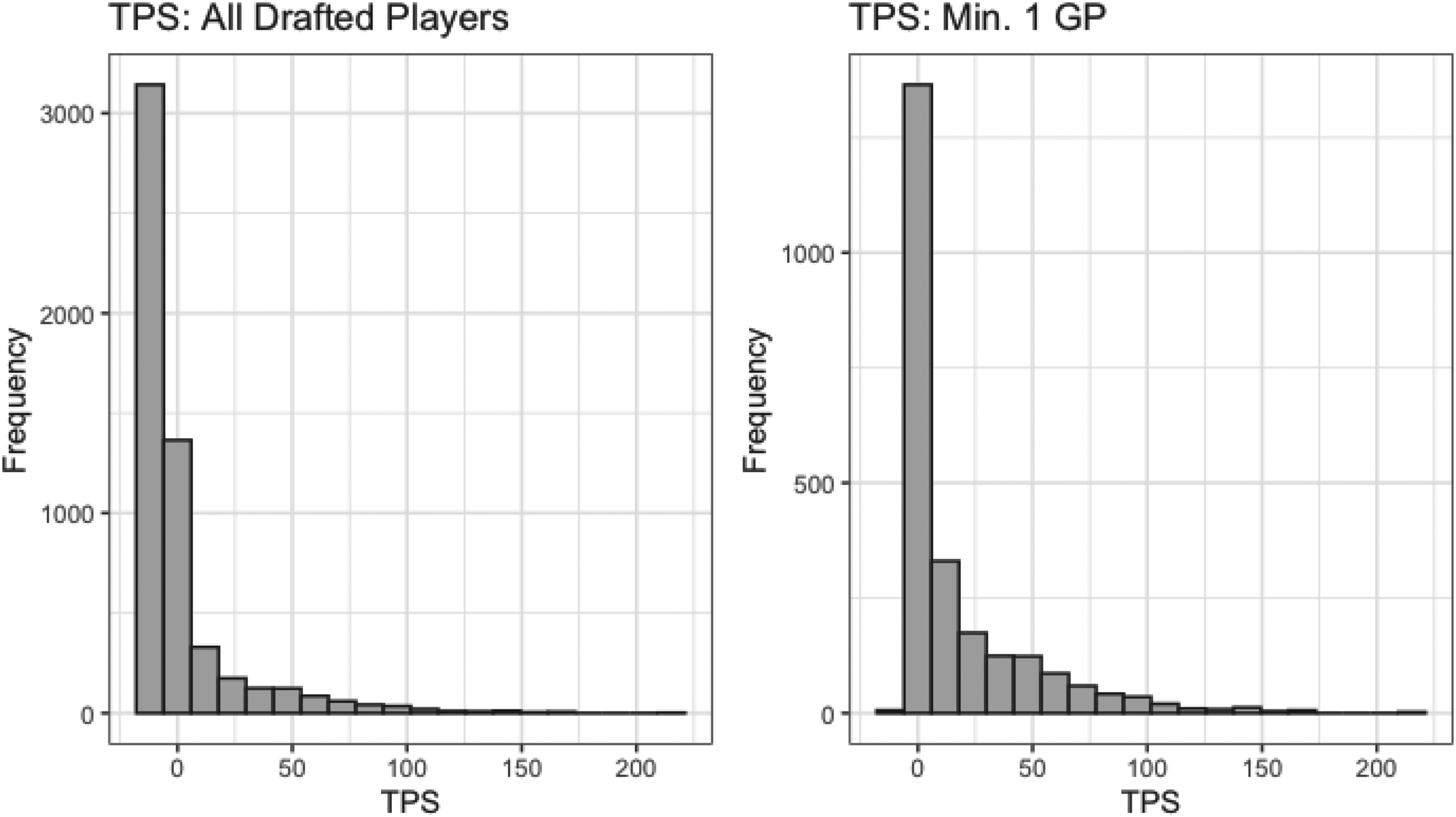
Figure 3 provides histograms of $Y_{3} = T P S = \sum_{s} A P S_{s}$ , where $A P S_{s}$ corresponds to APS in season $s$ , for all drafted players in our dataset. The distribution for all drafted players, and for players with at least one game played in the NHL are similar to the distributions of APS. Most of the players in the dataset are around zero, with a small number of elite players with high TPS.

Figure 3.

Histogram of total-point-share by all drafted players (left) and drafted players who played at least one NHL game (right).

Standardized salary ranking ( $Y_{4}$ )

The fourth measure of player value, $Y_{4}$ , is standardized-salary-ranking. We have specified this ranking as the percentile of the annual average value (AAV) of contracts for each player within each year. We denote this metric as PAAV. By using the percentiles instead of raw values of AAV we standardize the data since salaries will change over time with inflation. For example, in the 2016 season, there were 762 players under contract. Morgan Rielly of the Toronto Maple Leafs had an AAV of $5,000,000 in that season. This placed him in position 133 where the lowest AAV was $335,843 (Sven Andrighetto) and the highest salary was $10,500,000 (Jonathan Toews). Therefore, Rielly had a PAAV percentile ranking of 82.5.

This method of player value gives a different perspective than performance measures as salaries are determined by team executives. Performance measures surely play a role in how an executive views a players value, however, it is impossible to quantify everything that a team includes in defining player value. All of these underlying attributes will go into negotiating a player’s contract. This is the major benefit of using PAAV as a measure of player value. Another benefit is that PAAV captures brilliance over short-time spans versus measuring player value based on longevity.

A downside of using PAAV as a measure of player value is similar to the issue of games-played in Section Games-played ( $Y_{1}$ ), in which there may be a bias towards high draft picks playing more games than lower draft picks (Tingling, 2017). These same players who may be favoured by executives who drafted them high may also receive a bigger contract than a player drafted lower. Another downside to this valuation method occurs when players sign long term contracts with high AAV do not play to their potential, and in some cases even get bought out by the team. For example, Vincent Lecavalier was selected first overall by the Tampa Bay Lightning in the 1998 NHL Draft. After many good seasons with the Lightning, he was rewarded with a 11-year $85-million contract beginning in the 2009–2010 season. Shortly afterwards (in 2013), he was bought out, with the Lightning required to pay him until 2027. We note that the NHL salary cap was introduced in 2005, and therefore early years of our dataset will involve salaries not subject to a salary cap.

Comparison of valuation metrics

Having introduced the four valuation metrics $Y_{1}$ , $Y_{2}$ , $Y_{3}$ and $Y_{4}$ , it is worth asking whether there is an “ideal” metric. We believe that drafting objectives may be team specific. For example, consider a small-market team that is attempting to build a fan-base. In this case, player brilliance (for even a short period) may be preferred to solid but unspectacular longevity. One might therefore consider a modification to $Y_{2}$ (average-point-share) and $Y_{3}$ (total-point-share). Instead, maximum seasonal point-share may be preferable. Alternatively, a team that is doing well and is challenging for the Stanley Cup may want a player who can immediately put them over the top. In this case, a metric that focuses on immediate success may be preferable to $Y_{1}$ , $Y_{2}$ , $Y_{3}$ and $Y_{4}$ . It seems that one is only limited by their imagination in deriving metrics. However, all sensible metrics should be related to winning games, and we believe that all of $Y_{1}$ , $Y_{2}$ , $Y_{3}$ and $Y_{4}$ address winning.

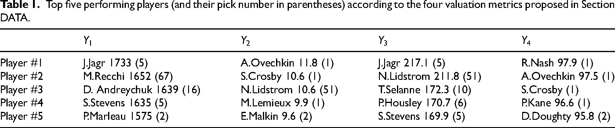
Table 1 provides the top five performing players according to the four valuation metrics along with their draft pick number. We observe that the proposed excellence metrics correspond to widely recognized top players. We also suspect that it is more difficult to predict which players excel with respect to the longevity metrics $Y_{1}$ (GP) and $Y_{3}$ (TPS). Accordingly, we see the draft pick numbers for $Y_{1}$ and $Y_{3}$ slightly larger than those for $Y_{2}$ and $Y_{4}$ .

Table 1.

Top five performing players (and their pick number in parentheses) according to the four valuation metrics proposed in Section DATA.

	$Y_{1}$	$Y_{2}$	$Y_{3}$	$Y_{4}$
Player #1	J.Jagr 1733 (5)	A.Ovechkin 11.8 (1)	J.Jagr 217.1 (5)	R.Nash 97.9 (1)
Player #2	M.Recchi 1652 (67)	S.Crosby 10.6 (1)	N.Lidstrom 211.8 (51)	A.Ovechkin 97.5 (1)
Player #3	D. Andreychuk 1639 (16)	N.Lidstrom 10.6 (51)	T.Selanne 172.3 (10)	S.Crosby (1)
Player #4	S.Stevens 1635 (5)	M.Lemieux 9.9 (1)	P.Housley 170.7 (6)	P.Kane 96.6 (1)
Player #5	P.Marleau 1575 (2)	E.Malkin 9.6 (2)	S.Stevens 169.9 (5)	D.Doughty 95.8 (2)

Functional data analysis

Basic model

Functional data analysis is an emergent research area in which wide-ranging methods have already been developed (Ramsay and Silverman, 2005). In a sentence, FDA extends regression techniques involving points to regression involving functions in a nonparametric fashion.

FDA functions can be defined along various axes, although time is a common and logical axis. For this reason, FDA is particularly well suited to applications in sport since there are many sporting events of interest that occur longitudinally in time. For example, it is natural to consider sporting functions which correspond to players and teams across time horizons such as matches and seasons. However, to date, there have been very few applications of FDA to sporting problems. Two exceptions are Chen and Fan (2018) who investigated the score differential process in basketball, and Guan et al. (2022) who predicted in-game match outcomes in the National Rugby League.

In this investigation, we have a response variable $y_{i j}$ which corresponds to the value of the $j$ th-picked player in year $i$ . We also have an independent variable $x_{i j} = j$ which is the player’s draft position (previously denoted as Pick). Recall that four candidate choices for $y_{i j}$ are described in Sections Games-played ( $Y_{1}$ )–Standardized salary ranking ( $Y_{4}$ ). With the aforementioned data, one might consider the following linear regression model as a baseline model

y_{i j} = α_{i} + β_{i} x_{i j} + ϵ_{i j}

(1)

where the

ϵ_{i j}

terms are assumed independent and arise from a normal distribution with zero mean and constant but unknown variance.

In this application, there are some immediate questions related to the assumptions of the linear regression model (1). First, the linearity assumption relating player value and draft position in equation (1) is highly questionable. In fact, all previous work has indicated that the value of draft picks has an exponential shape which tends to flatten towards the end of the draft. Second, the distributional assumptions associated with $ϵ_{i j}$ appear strong. For example, with the games played metric $Y_{1}$ , one might expect skewness in $ϵ_{i j}$ for players selected late in the draft. The reason for this is that they either do not produce (zero value as expected for a late round pick) or they surprise positively. Third, although model (1) has an intercept and slope parameter which varies across years, it does not account for similarities amongest years. Yearly differences are expected since some draft years are stronger/weaker in player talent. Model (1) is a regression of points and does not take into account the functional form of the data across years. Fortunately, the FDA model which we propose addresses the above shortcomings.

Proposed model

Functional linear regression

The proposed FDA model addresses some of the shortcomings described in Section Basic model. We consider the model

y_{i j} = α_{i} + β_{i} x_{i} (j) + ϵ_{i j}

(2)

where

x_{i} (j)

is a nonparametric function evaluated at pick

j

. We observe that model (2) has a functional regression form, following the form of model (1), and the

ϵ_{i j}

terms are assumed independent and arise from a normal distribution with zero mean and constant but unknown variance. As mentioned in Section Basic model, we do not want to do regression of points, so we use this functional form of the data across years to address the yearly differences.

Introducing monotonicity in our model ensures we follow the assumption that on average, an earlier pick number is always more valuable than a later pick number. For example, we want to impose the condition that the 10th draft pick is more valuable than the 11th draft pick, on average. To restrict our functions to be monotonically decreasing in 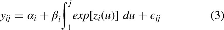$j$ , we re-parameterize our function $x_{i} (j) = - \int_{1}^{j} e x p [z_{i} (u)] d u$ which causes $x_{i} (j)$ to be decreasing in $j$ . The resulting model is written as

y_{i j} = α_{i} + β_{i} \int_{1}^{j} e x p [z_{i} (u)] d u + ϵ_{i j}

(3)

and the fitted function for

y_{i j}

is monotonically decreasing in

j

provided

β_{i} > 0

Basis functions

As stated in Section Basic model, the linearity assumption relating to player value is highly questionable. In our proposed model we address this issue and introduce nonlinearity through the use of basis-functions. Basis-functions, are denoted by 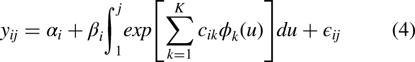$ϕ_{k}$ where $k = 1, \dots, K$ , are functional building blocks that allow a curve to act differently between break-points. These basis-functions make up each $z_{i} (u)$ in model (3), and are defined by a basis-function-expansion of the form $z_{i} (u) = \sum_{k = 1}^{K} c_{i k} ϕ_{k} (u)$ , where the $c_{i k}$ are expansion coefficients. Inserting our basis-functions into equation (3) results in

y_{i j} = α_{i} + β_{i} \int_{1}^{j} e x p [\sum_{k = 1}^{K} c_{i k} ϕ_{k} (u)] d u + ϵ_{i j}

(4)

Our proposed model uses B-spline basis-functions. B-splines are piece-wise polynomials that are flexible. To produce a B-spline basis, we need to specify knots and break-points in our functions. We will only use a single knot at each break point. As the number of knots grows, so does the variability of the resulting curves. Our goal is to find the optimal amount of knots that produces a smooth curve without losing information about variability. For our model, we will use an order four cubic-spline basis with a single knot at each break point. This method ensures all neighbouring splines will have matching first and second derivatives, resulting in a smooth continuous curve.

The number of knots specified determines the number of $K$ basis-functions. Too many basis-functions will result in over-fitting, and a high measurement error, whereas too few basis-functions will fail to capture the features of the curve. We desire a smooth curve that provides interpretability. This is also know as bias-variance trade-off. Typically an optimal $K$ is chosen by minimizing mean-squared-error (MSE), which is common way to deal with the bias-variance trade-off. However, since we want the resulting mean curve to be smooth, we use fewer knots than optimal. We fit by eye, increasing the number of knots until wiggles appeared.

Smoothing

Now that we have specified our model (4), we can define the smoothing technique. Our linear smoother is obtained by determining the coefficients of the basis-expansion, $c_{i k}$ . We estimate these coefficients with a penalized weighted least squares criterion (PENSSE). This criterion includes a smoothing parameter, $λ$ , where as $λ$ increases, the roughness penalty is larger and $y_{i j}$ becomes more linear and as $λ$ decreases, the penalty is reduced and $y_{i j}$ fits the data better. The details of the PENSSE criterion are provided in Ramsay and Silverman (2002).

Final model

Estimates for 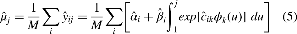${\hat{α}}_{i}$ , ${\hat{β}}_{i}$ , and ${\hat{c}}_{i k}$ for each ${\hat{y}}_{i j}$ from model (4) are computed with the fda R package (Ramsay et al., 2022). These estimates are derived through an iterative process that minimise the PENSSE as described in Section Smoothing. After determining ${\hat{y}}_{i j}$ for all draft years, $i$ , the resulting mean curve for draft position $j$ is defined as

{\hat{μ}}_{j} = \frac{1}{M} \sum_{i} {\hat{y}}_{i j} = \frac{1}{M} \sum_{i} [{\hat{α}}_{i} + {\hat{β}}_{i} \int_{1}^{j} e x p [{\hat{c}}_{i k} ϕ_{k} (u)] d u]

(5)

where

M

is the total number of draft years, or functions, in the analysis.

Model (4) is perhaps one of the most basic models that has been developed in FDA, but is of great practical importance.

Model (4) may be viewed as nonparametric (or perhaps more accurately, semiparametric) and therefore shares similarities with the approach taken by Schuckers (2011b) which uses a loess function for smoothing. One advantage that we see in the FDA approach is the simple implementation of monotonicity in the average pick value curve. Also, there is a difference in approach between regressing functions (e.g. the pick value curve for a year) as is done in FDA versus regressing points using loess (e.g. all pick values for a given year). In the latter, there is no consideration of the structure between adjacent picks in a given year. This may be important when some draft years are stronger than other draft years.

In our criticism of the basic linear regression model (1), we point out that there may be error skewness in the data which violates the assumption that $ϵ_{i j} \sim Normal (0, σ^{2})$ . In fact, our simple FDA model (4) also does not address this limitation. We do note that more complex FDA models Liu et al. (2021) consider these issues. In addition, we pointed out that the simple linear regression approach does not take into account the similarity between curves from different draft years. Although the proposed approach specified by model (4) also fails to account for similarity, more complex FDA models consider the relationship between curves (Cao and Ramsay, 2010). It may also have been appropriate to introduce strategies to deal with zero-inflation with respect to the four outcome metrics as is done in Woolford (2021).

Results

We now explore the results of our proposed FDA model for the four measures of player value described in Section Games-played ( $Y_{1}$ )–Standardized salary ranking ( $Y_{4}$ ). Computing was done in R and followed the methods provided in Ramsay et al. (2009).

Pick value charts

We define each draft year, $i$ , as a function of the overall pick in the draft, $j = 1, \dots, 224$ . As discussed in Section DATA we truncate any draft with more than 224-picks to represent the current state of the NHL draft. For each measure of player value we will show the mean curve and 95% pointwise confidence interval. The inclusion of confidence intervals have not been included in other pick value charts but we believe it is a valuable addition to our charts. We then validate our model with a cross-validation method and compare our results.

Games-played ( $Y_{1}$ )

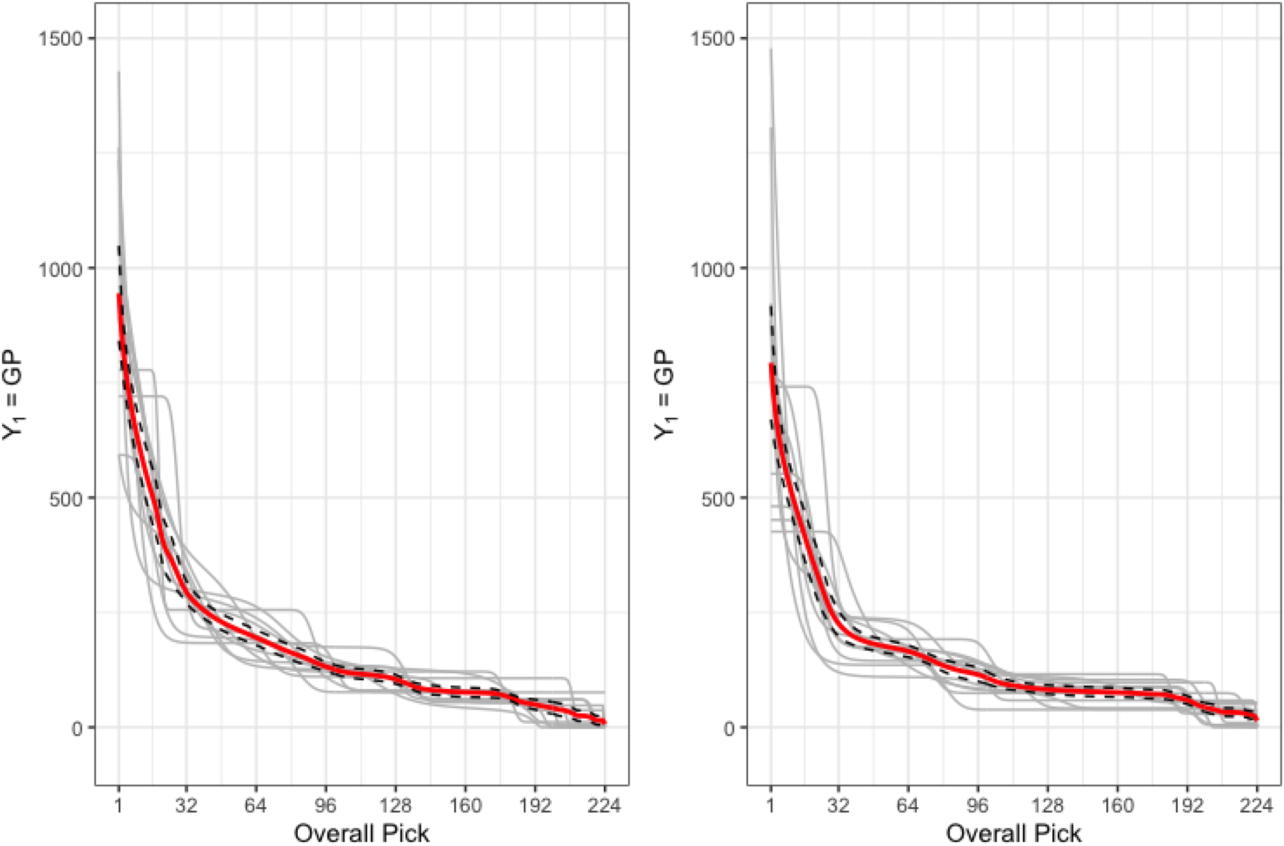
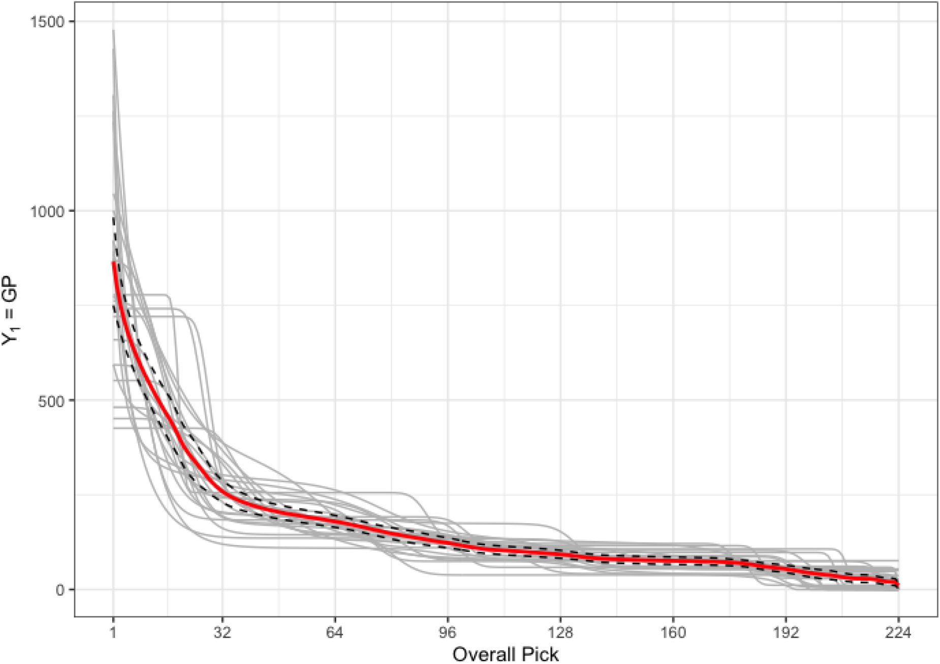
Figure 4 provides the predicted curves, ${\hat{y}}_{i j}$ , for draft years $i = 1982, 1983, \dots, 2006$ and the mean curve, ${\hat{μ}}_{j}$ , for the first measure of player value GP ( $Y_{1}$ ). The mean curve represents the predicted number of GP we would expect from a player drafted at pick $j$ . For instance, we predict that a player drafted in 1st-overall should play 866 games in the NHL, compared to a player drafted 33rd-overall (1st pick of the 2nd-round) who we predict should play 252 games. This sharp decline in value is apparent for the first-round (picks 1–32), followed by the curve flattening out with a much slower decrease.

Figure 4.

Plot of the measure of player value, GP. Shown are predicted curves, ${\hat{y}}_{i j}$ , for draft years 1982-2006 (grey) and the resulting mean curve, ${\hat{μ}}_{j}$ , and pointwise confidence interval (red) for overall picks 1–224.

Figure 4 also shows the 95% pointwise confidence interval for ${\hat{μ}}_{j}$ . The interval is the largest for picks 1–32, and gets smaller as overall pick increases. This shows the large variation of player value from the early stage of the draft, whereas players drafted late in the draft are unlikely to provide much value at all.

Average point share ( $Y_{2}$ )

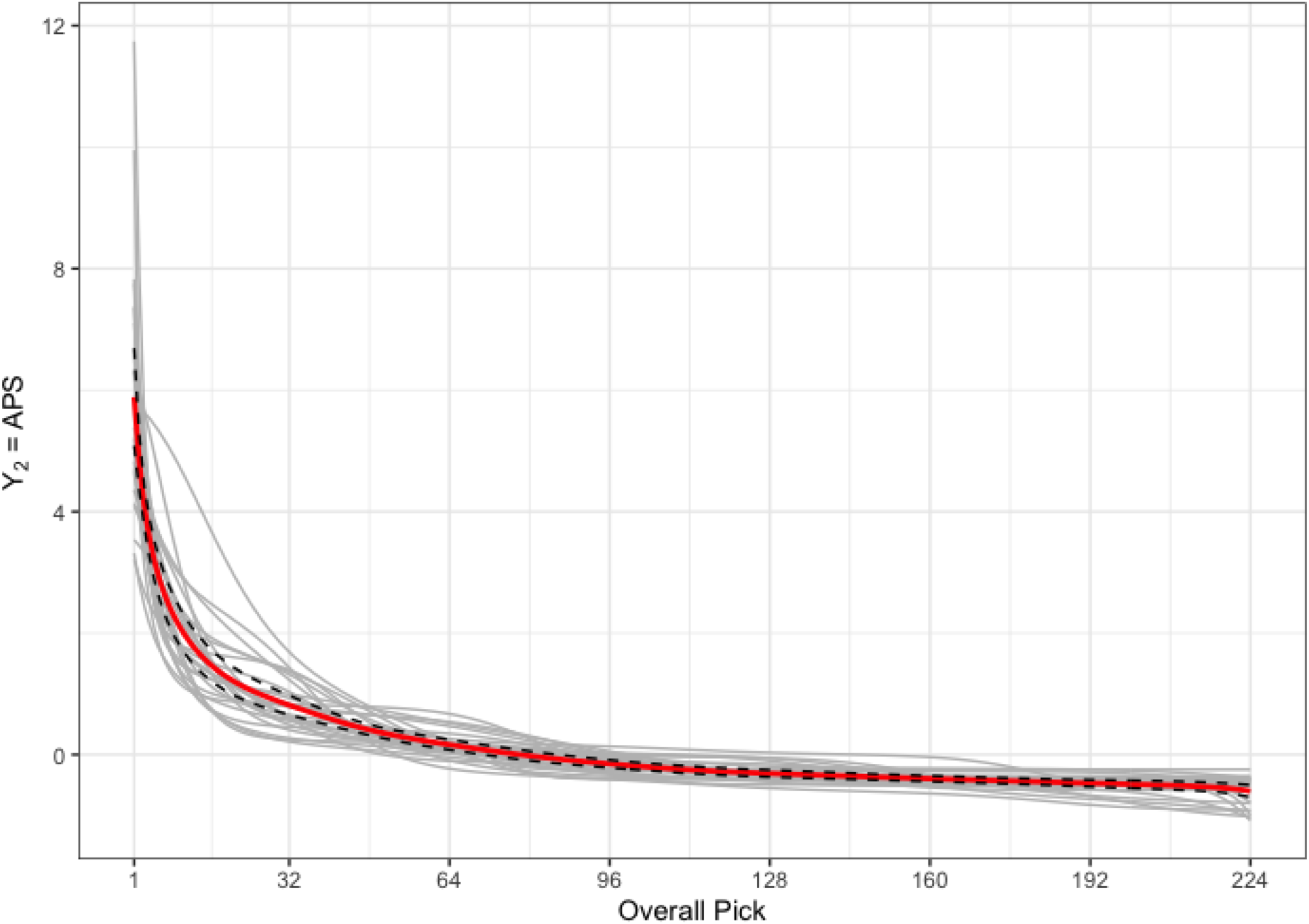
Figure 5 provides the predicted curves, ${\hat{y}}_{i j}$ , for draft years $i = 1982, 1983, \dots, 2006$ and the mean curve, ${\hat{μ}}_{j}$ , for the second measure of player value APS ( $Y_{2}$ ). The mean curve represents the predicted APS we expect a player drafted at pick $j$ during their career. We predict that the 1st-overall pick should have an APS of 5.67, and players drafted with the 87th pick or later to have an APS below 0.

Figure 5.

Plot of the measure of player value, APS. Shown are predicted curves, ${\hat{y}}_{i j}$ , for draft years 1982-2006 (grey) and the resulting mean curve, ${\hat{μ}}_{j}$ , and pointwise confidence interval (red) for overall picks 1–224.

Examining the 95% pointwise confidence interval in Figure 5 shows that players drafted early in the draft are predicted to provide value, but there is lots of variation in this prediction. We can also see that it is very likely that players drafted 50th or later are unlikely to provide much value over their careers. We observe less variation in APS than in GP.

Total point share ( $Y_{3}$ )

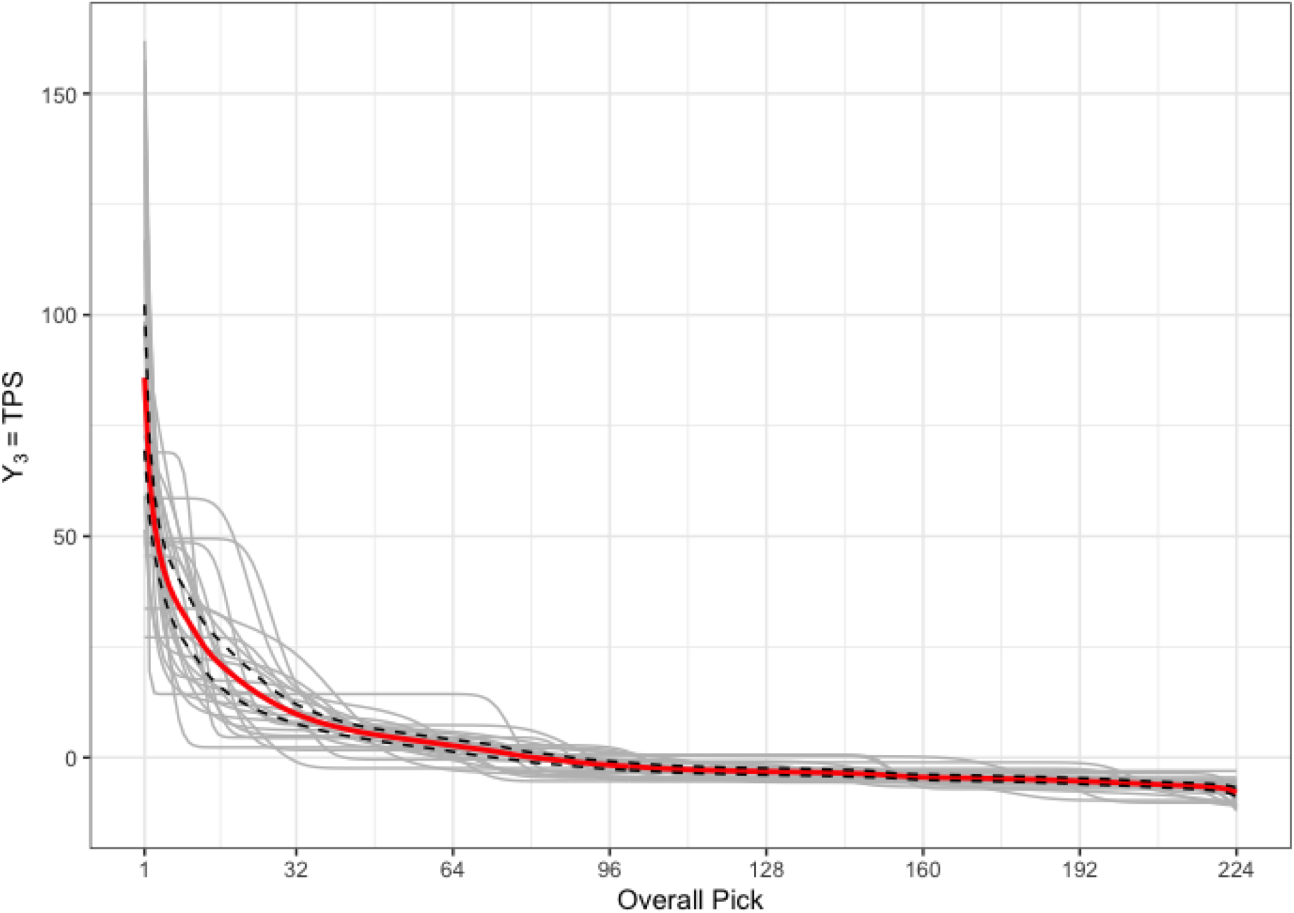
Figure 6 provides the predicted curves, ${\hat{y}}_{i j}$ , for draft years $i = 1982, 1983, \dots, 2006$ and the mean curve, ${\hat{μ}}_{j}$ , for the third measure of player value TPS ( $Y_{3}$ ). The mean curve represents the total APS we expect a player drafted at pick $j$ to have over their career. We predict that the 1st-overall pick should have 83.67 TPS, and players drafted with the 90th pick or later should have a TPS below 0.

Figure 6.

Plot of the measure of player value, TPS. Shown are predicted curves, ${\hat{y}}_{i j}$ , for draft years 1982–2006 (grey) and the resulting mean curve, ${\hat{μ}}_{j}$ , and pointwise confidence interval (red) for overall picks 1–224.

The 95% pointwise confidence interval in Figure 6 is similar to the confidence interval in Figure 5. However, the variation for early picks is larger for TPS than it is for APS. We can attribute this larger variation to the difference in career length across players. If two players have similar APS, the player who plays more games in the NHL will have a larger TPS than the player with fewer games.

Standardized salary ranking ( $Y_{4}$ )

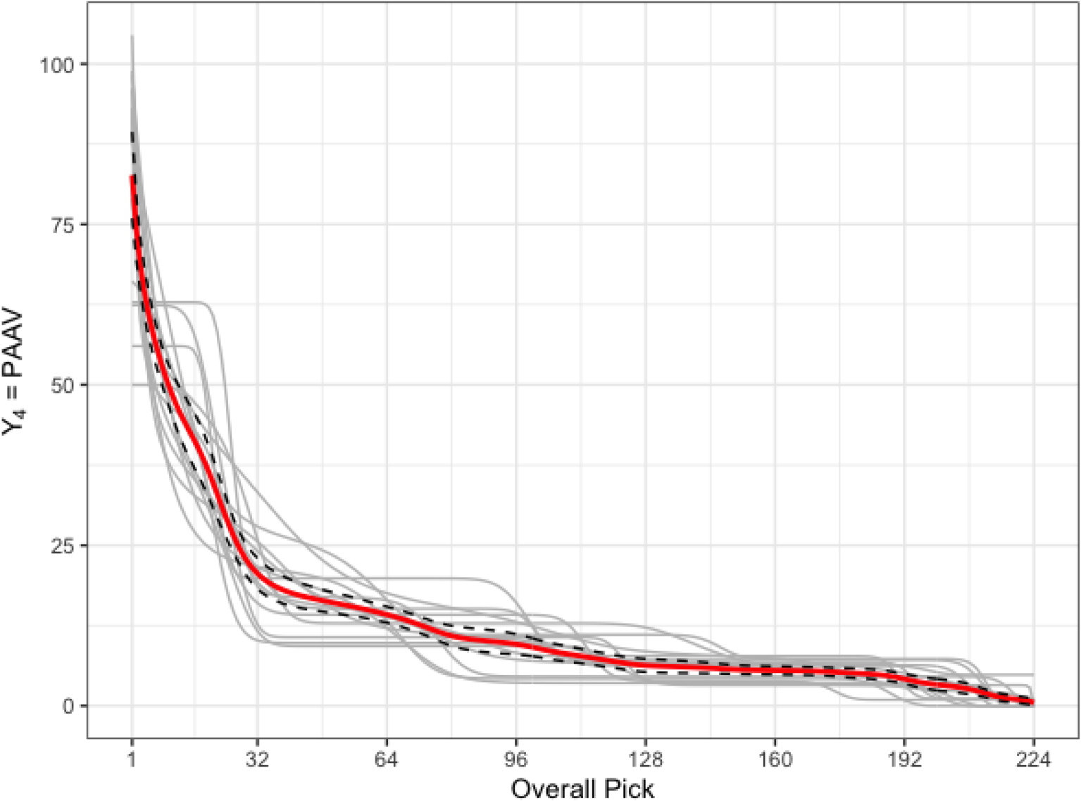
Figure 7 provides the predicted curves, ${\hat{y}}_{i j}$ , for draft years $i = 2001, 2002, \dots, 2016$ and the mean curve, ${\hat{μ}}_{j}$ , for the third measure of player value PAAV ( $Y_{4}$ ). The mean curve represents the predicted percentile of AAV that a player drafted at pick $j$ should average over their career. We predict that the 1st overall pick should average being in the 82nd percentile of AAV over their career, and players drafted with the 10th pick or later are predicted to be in the 50th percentile or lower.

Figure 7.

Plot of the measure of player value, PAAV. Shown are predicted curves, ${\hat{y}}_{i j}$ , for draft years 2001–2016 (grey) and the resulting mean curve, ${\hat{μ}}_{j}$ , and pointwise confidence interval (red) for overall picks 1–224.

The 95% pointwise confidence interval in Figure 7 shows relatively high variation up to pick 100, and very high variation for early picks.

Comparing value charts

To compare the four measures of player value, we can visualize the corresponding mean curves on one plot. Since all the measures of player value are in different scales, we first need to standardize them. To do this we set the value for ${\hat{y}}_{i 1} = 1000$ by multiplying the original ${\hat{y}}_{i 1}$ by a constant. We then multiply all other values for $j = 2, 3, \dots, 224$ by this same constant to get a set of standardized values.

Figure 8 shows these standardized mean curves for the four measures of player value. The mean curves for APS and TPS are quite similar, with the small difference of APS being smoother. We also see that the mean curves for GP and PAAV are similar, and place a higher value overall compared to APS and TPS. This is likely due to GP and PAAV being non-performance based measures since there is a smaller gap between the top players and mid-tier players for these measures. Comparing the measures for longevity, GP and TPS, against the measures for excellence, APS and PAAV, there is not a substantial enough difference to make conclusions.

Figure 8.

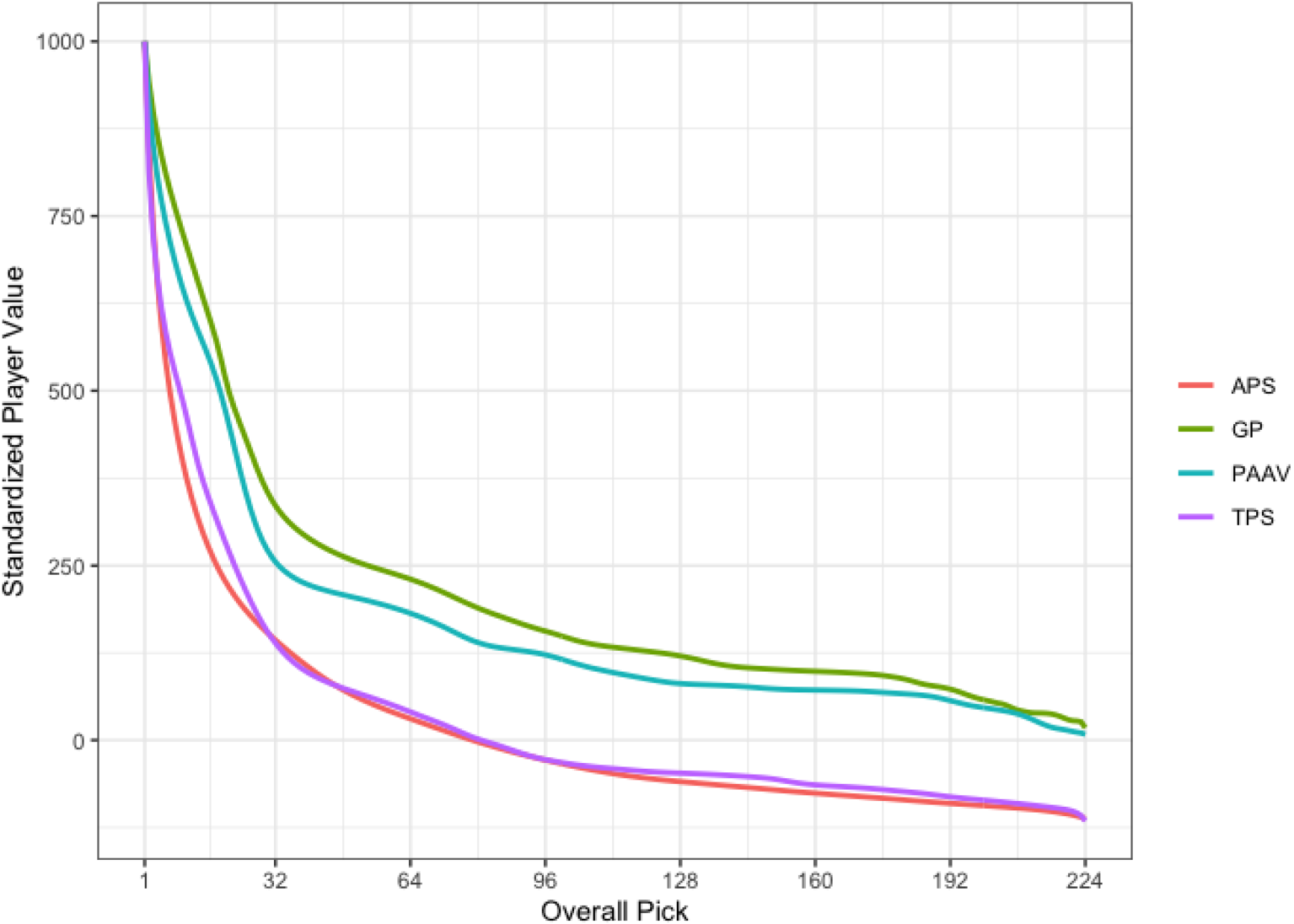
Plot of mean curves from all measures of player value, $Y_{1}, Y_{2}, Y_{3}, Y_{4}$ . Values are standardized so that the value for the 1st-overall pick $Y_{i 1} = 1000$ .

Validation

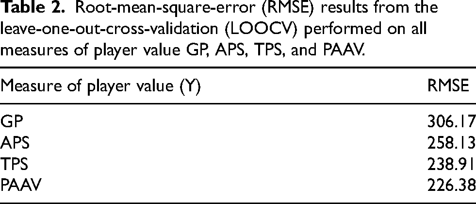
We validate our model with a leave-one-out-cross-validation (LOOCV) for each measure of player value. This method involves taking one draft year out as a test year and completing the analysis, then repeating the process for all draft years in the dataset. We calculate the root-mean-square-error (RMSE) for each test year with the corresponding predicted values and take the average RMSE from all iterations. The RMSE for year $i$ is defined as $\frac{1}{n_{j}} \sum_{j = 1}^{n_{j}} (y_{i j} - {\hat{y}}_{i j})^{2}$ . The standardized values described in Section Comparing value charts are used for this process so the RMSE for each measure has the same scale. Table 2 contains the resulting RMSE from LOOCV. Our results show that $Y_{4} =$ PAAV performed best while GP was the worst in terms of predictive error. The high RMSE for GP may be due to the issues described in Section Games-played ( $Y_{1}$ ) about injuries, and that many players who do not have a high APS, TPS, or PAAV may still be able to have a long career if they are valuable in other aspects. The low RMSE for PAAV is likely because this measure is not affected by injury or decrease in production during a contract. Top draft picks that sign big contracts who do not meet expectations are not penalized in this measure until they sign a new contract. Perhaps it is not a coincidence that the pick value chart based on $Y_{4} =$ PAAV (Figure 8) lies between the charts based on $Y_{1} =$ GP and the two point share charts ( $Y_{2} =$ APS and $Y_{3} =$ TPS).

Table 2.

Root-mean-square-error (RMSE) results from the leave-one-out-cross-validation (LOOCV) performed on all measures of player value GP, APS, TPS, and PAAV.

Measure of player value (Y)	RMSE
GP	306.17
APS	258.13
TPS	238.91
PAAV	226.38

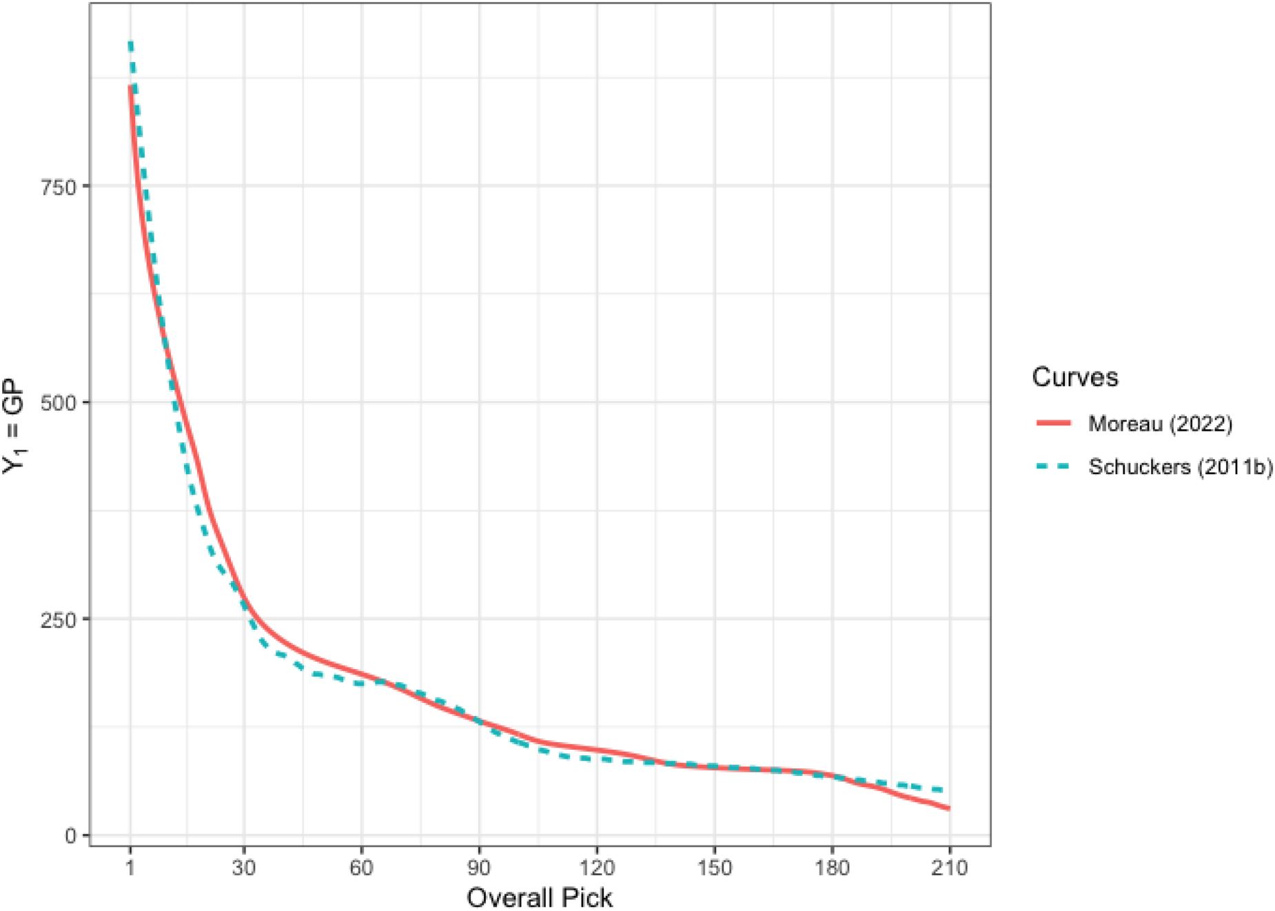
We also investigate our model by comparing the most widely used measure of player value, GP, to the results from Schuckers (2011b), which includes predictions for the number of career GP we expect for draft picks from $j = 1, 2, \dots, 210$ . Figure 9 shows the mean curves for each method.

Figure 9.

Comparison of predicted mean curves for GP from our derived model (5) and Schuckers (2011b) for draft picks 1–210.

We see the curve from Schuckers (2011b) is closely related to the one derived in this paper. Schuckers curve is not strictly monotonically decreasing, which was stressed as an important property of our proposed model. Besides that, it does not seem that FDA has provided much of a difference.

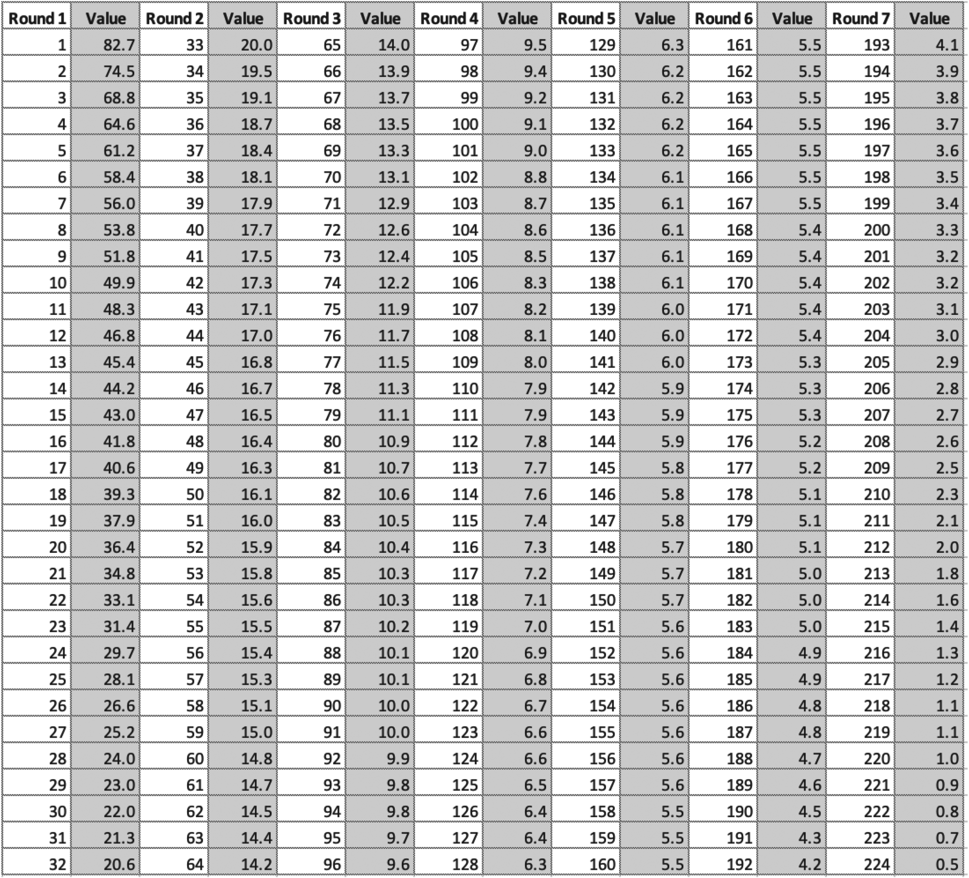
Having identified $Y_{4} = P A A V$ as the preferred valuation metric according to Table 2, we compare actual valuations versus expected valuations (based on pick number). Table 3 provides the top five and bottom five players according to this criterion. We observe that the players who excelled above their expected valuations (first column) could be considered “steals” as they were all late round picks. On the other hand, the “busts” (column 2) correspond to players who were evaluated highly and drafted early. Figure 10 provides the numerical entries for the pick value chart based on $Y_{4} =$ PAAV.

Figure 10.

Numerical entries for the pick value chart based on the preferred metric $Y_{4} =$ PAAV.

Table 3.

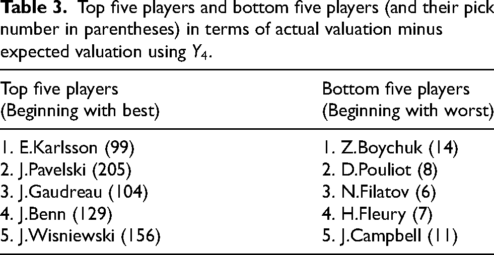
Top five players and bottom five players (and their pick number in parentheses) in terms of actual valuation minus expected valuation using $Y_{4}$ .

Top five players	Bottom five players
(Beginning with best)	(Beginning with worst)
1. E.Karlsson (99)	1. Z.Boychuk (14)
2. J.Pavelski (205)	2. D.Pouliot (8)
3. J.Gaudreau (104)	3. N.Filatov (6)
4. J.Benn (129)	4. H.Fleury (7)
5. J.Wisniewski (156)	5. J.Campbell (11)

In the NHL pick value chart literature, there does not seem to be any studies of how value metrics have changed over time. Amongst the metrics $Y_{1}, \dots Y_{4}$ , it seems that the games played metric $Y_{1}$ may be the most sensitive to time changes. For example, one could imagine that sports science contributions in terms of nutrition and condition may have increased longevity. To investigate this, in Figure 11, we provide two pick value charts based on $Y_{1}$ . The first is based on data for players drafted in the period 1982–1993, and the second is based on the period 1994–2006. We observe little difference in the two charts.

Figure 11.

Pick value charts for the games played metric $Y_{1}$ . The first chart is based on players drafted in the time period 1982–1993 and the second chart is based on data from the time period 1994–2006.

Discussion

In this paper we develop valuation measures for draft picks in the NHL entry draft and analyze the value of each pick with these measures. We use FDA to find a mean value curve from many observed functions using a nonparametric approach. This approach allows us to use a functional linear regression framework that introduces nonlinearity to account for the differences of players across draft years. The four measures of player value used are games-played (GP), average-point-share (APS), total-point-share (TPS), and a standardized salary ranking (PAAV). The resulting mean value curve for each measure is the predicted value of a player drafted at a certain overall draft pick.

There are limitations to the proposed methods. Limitations of the measures of player value differ by measure, but include accounting for injuries, draft pick bias, and confounding variables such as teammates. Also, for GP, APS, and TPS, we are limited to using data only up until 2006. Surely the NHL has developed and changed over time, so not being able to use recent data may limit our accuracy when comparing our results to the present day. There is also a lack of reported salary data before 2001, and including more data may be beneficial to our results.

Although comparing many measures of player value is useful to determine differences, having a mean value curve from an all encompassing metric would be very useful. Developing one metric from a combination of many metrics and then using our proposed model would be an area of future work which we would like to explore.

Our draft value charts can be useful tools for NHL teams. They can be used as a trade tool, to determine a fair value when trading draft picks with another team. They can also be used as a salary-cap tool, to predict the contract value of a drafted player years in advance of signing.

Footnotes

Funding

The authors disclosed receipt of the following financial support for the research, authorship, and/or publication of this article: R. Moreau is an MSc graduate, H. Perera is Senior Lecturer and T. Swartz is Professor, Department of Statistics and Actuarial Science, Simon Fraser University, 8888 University Drive, Burnaby BC, Canada V5A1S6. Swartz (tswartz@sfu.ca) has been partially supported by the Natural Sciences and Engineering Research Council of Canada. The work has been carried out with support from the CANSSI (Canadian Statistical Sciences Institute) Collaborative Research Team (CRT) in Sports Analytics. The authors thank four anonymous Reviewers whose comments have improved the manuscript.

Declaration of conflicting interests

The authors declared no potential conflicts of interest with respect to the research, authorship, and publication of this article.

References

Bell

(2022) The worst first-overall draft picks in NHL history. Available at: https://thehockeywriters.com/the-worst-nhl-draft-picks/ (accessed 18 October 2022).

Cacchione

(2018) MLB rule IV draft: Valuing draft pick slots. Masters Thesis in the Department of Economics, City College of New York. Availabel at: https://academicworks.cuny.edu/cgi/viewcontent.cgi?article=1759&context=cc_etds_theses (accessed online 12 September 2022).

Cao

Ramsay

(2010) Linear mixed effects modeling by parameter cascading. Journal of the American Statistical Association 105(489): 365–374.

Chen

Fan

(2018) A functional data approach to model score difference process in professional basketball games. Journal of Applied Statistics 45(1): 112–127.

Guan

Nguyen

Cao

Swartz

(2022) In-game win probabilities for the National Rugby League using tracking data. The Annals of Applied Statistics 16(1): 349–367.

Kubatko

(2010) Calculating point shares. Available at: https://www.hockey-reference.com/about/point_shares.html (accessed 18 October 2022).

Liu

Wang

Nie

Cao

(2021) Semiparametric mixed-effects ordinary differential equation models with heavy-tailed distributions. Journal of Agricultural Biological and Environmentatl Statistics 26: 428–445.

Massey

Thaler

(2013) The loser’s curse: Decision making and market efficiency in the national football league draft. Management Science 59(7): 1479–1495.

Moskowitz

Wertheim

(2011) Scorecasting: The Hidden Influences Behind how Sports are Played and Games are Won. New York: Crown Archetype.

10.

Pelton

(2017) Draft pick trade value chart - 2017 version. nbasense, Availabel at: http://nbasense.com/draft-pick-trade-value/2/kevin-pelton-2 (accessed 12 September 2022).

11.

Ramsay

Hooker

Graves

(2009) Functional Data Analysis with R and MATLAB. New York: Springer-Verlag.

12.

Ramsay

Hooker

Graves

(2022) Functional Data Analysis R Package ’fda’. CRAN.

13.

Ramsay

Silverman

(2002) Applied Functional Data Analysis: Methods and Case Studies. New York: Springer-Verlag.

14.

Ramsay

Silverman

(2005) Functional Data Analysis, 2nd Edition. New York: Springer Series in Statistics, Springer.

15.

Schuckers

(2011a) An alternative to the NFL draft pick value chart based upon player performance. Journal of Quantitative Analysis in Sports 7(2): 10.

16.

Schuckers

(2011b) What’s an NHL draft pick worth? A value pick chart for the national hockey league. Availabel at: https://myslu.stlawu.edu/msch/sports/Schuckers_NHL_Draft.pdf (accessed online 12 September 2022).

17.

Swartz

Arce

Parameswaran

(2013) Assessing value of the draft positions in major league soccer’s superdraft. The Sport Journal 16: 9.

18.

Spotrac (2022) [Data File]. Availabel at: https://www.spotrac.com/ (accessed 28 October 2022).

19.

Sports Reference LLC (2022) Stathead Hockey [Data File]. Availabel at: https://stathead.com/hockey/ (accessed 18 October 2022).

20.

Tingling

(2017) Educated guesswork: Drafting in the national hockey league. In: Albert JA, Glickman ME, Swartz TB and Koning RH (eds) Handbook of Statistical Methods for Design and Analysis in Sports. Boca Raton: Chapman & Hall/CRC Handbooks of Modern Statistical Methods, pp.327–339.

21.

Vollman

(2018) NHL Player Data 1967–2018 [Data File]. Availabel at: http://www.hockeyabstract.com/testimonials (accessed 18 October 2022).

22.

Woolford

Dean

Martell

Cao

Wotton

(2021) Lightning-caused forest fire risk in Northwestern Ontario, Canada is increasing and associated with anomalies in fire-weather. Environmetrics 25: 406–416.

Valuation of NHL draft picks using functional data analysis

Abstract

Keywords

Introduction

DATA

Measures of player value

Games-played ( Y 1 )

Average point share ( Y 2 )

Total point share ( Y 3 )

Standardized salary ranking ( Y 4 )

Comparison of valuation metrics

Functional data analysis

Basic model

Proposed model

Functional linear regression

Basis functions

Smoothing

Final model

Results

Pick value charts

Games-played ( Y 1 )

Average point share ( Y 2 )

Total point share ( Y 3 )

Standardized salary ranking ( Y 4 )

Comparing value charts

Validation

Discussion

Footnotes

Funding

Declaration of conflicting interests

References

Games-played ( $Y_{1}$ )

Average point share ( $Y_{2}$ )

Total point share ( $Y_{3}$ )

Standardized salary ranking ( $Y_{4}$ )

Games-played ( $Y_{1}$ )

Average point share ( $Y_{2}$ )

Total point share ( $Y_{3}$ )

Standardized salary ranking ( $Y_{4}$ )