The First 110 Years of Laboratory Automation

Abstract

Prior to the widespread availability of electronic components after the Second World War, laboratory automation was constructed by end users and designed for specific tasks, mostly filtration, percolation, and washing operations. The earliest mention of automation in the chemical literature of the United States was in 1875, announcing a device to wash filtrates unattended. In the years that followed, a small number of commercial automated devices were sold, including large grinders for the preparation of coal samples. Around 1900, power stations began adopting automated carbon dioxide analysis. The development of electrical equipment for conductivity measurements enabled the first commercial, automated gas detection instruments for laboratory and field use around the time of the First World War. The growth of industrial production in the 1920s led to a desire for automated testing equipment, and the growing rubber industry was among the more successful early adapters. Photoelectric cells were first used in the early 1930s to create automatic titrators, and by the 1950s, automatic titration encompassed coulometric, potentiometric, and photometric devices. Combinations of chart recorders, photocells, and timers created other types of automated equipment such as stills and fraction collectors. The first true stand-alone automation for the laboratory included clinical chemistry analyzers, introduced during the 1950s.

Introduction

Laboratory automation today is a complex integration of robotics, computers, liquid handling, and numerous other technologies. For more than a century, the underlying reasons to automate have remained essentially unchanged: to save time and to improve performance through the elimination of human error. In the past, as is often the case today, the growth of certain industries or the demands of specific analytical challenges became the focal point for technological efforts. It is often the end-user or bench scientist who has seen the need for automation and been the driving force for the creation of an amazing array of devices. During the late 1800s, the seemingly simple tasks of washing a filtrate on a piece of filter paper and performing a solvent extraction were the first routine tasks to be automated. But new industries create new demands for new laboratory technologies. At the end of the 1800s, the growth of electrical generation and a better understanding of combustion processes revolutionized power generation. Automated chemical analyses soon found their way into the power plant. During the First World War, the need for rapid gas analysis prompted the development of the first commercially produced, automated laboratory devices. The descendents of these devices are now used to detect chemical weapons in times of conflict and pollution in peacetime. During the 1920s, as industry grappled with the problem of pH measurement and control, laboratory and process automation found their way into the sugar and paper industries. During the same decade with the growth of the automobile, the rubber industry was among the first to embrace laboratory automation.

The common factor in almost all contemporary laboratory automation is some combination of the microprocessor and personal computer. Automated systems can take many forms and serve many functions, but they are almost entirely built around the microprocessor. But before this technology became widely available, there was never a single automation-enabling device to be found in all systems. Components common to many devices included chart recorders, electrodes, potentiometers, Wheatstone bridges, siphons, motors, and photocells. The progression of technologies described in this article serves as reminder that the cutting-edge technologies of one generation become the routine tools of the next.

Until the 1950s, the vast majority of automation was designed and often built by the end-users. They used a wide variety of improvised components, hand-blown glass pieces, and, as they became available, commercial electronic components ( Table 1 ). With a few notable exceptions, systems sold as stand-alone automated devices did not appear until the 1950s. Transistors, reliable commercial electrodes, and electron multiplier tubes made the creation of automated devices by laboratory equipment suppliers practical. What was an engineering challenge for one generation of scientists frequently became off-the-shelf technology for the next.

Table 1.

Number of Citations with the Word Automatic in the Title Indexed by the American Chemical Society, divided by decade and the type of device (pressure regulator or gas generator) or the technology (electrodes, pumps, photocells) that enabled the device to operate automatically

	Siphon or Float	Regulation of Gas/Liquid Pressure or Temperature	Gas Generation	Conductivity	Mechanical Pumps	pH Electrodes	Other Types of Electrodes	Photocell
1879–1890	0	0	0	0	0	0	0	0
1891–1900	2	0	0	0	0	0	0	0
1901–1910	5	0	2	0	0	0	0	0
1911–1920	10	4	0	4	0	0	0	0
1921–1930	10	9	2	2	0	0	0	1
1931–1940	13	9	2	2	0	0	0	1
1941–1950	10	9	0	1	4	2	7	5
1951–1960	6	0	22	2	3	3	28	19

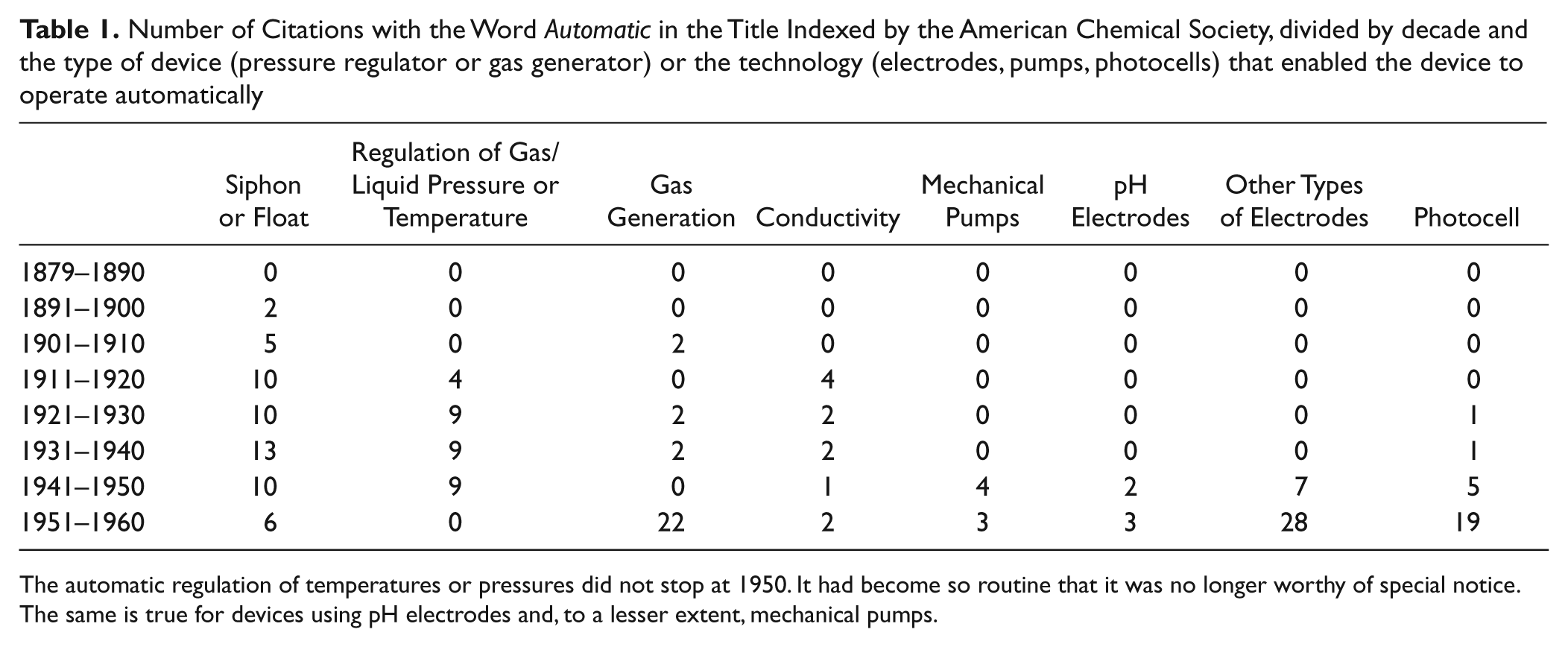
The automatic regulation of temperatures or pressures did not stop at 1950. It had become so routine that it was no longer worthy of special notice. The same is true for devices using pH electrodes and, to a lesser extent, mechanical pumps.

Siphons and Drips in a World Running on Coal, 1875–1920

The first mention of any automated device in the American chemical literature was in 1875 by Thaddeus M. Stevens, MD, professor of analytical chemistry at the College of Physicians and Surgeons of Indiana. His device was designed to drip water through a piece of filter paper at a controlled rate to wash a filtrate. It consisted of a sealed wash solution reservoir into which air was admitted through a controlled aperture. The larger the aperture, the faster the wash liquid would drip out of the bottom and pass through the filter paper. Stevens did not claim complete originality for the idea, stating that sealed vessels with a controlled drip rate had been developed by others. He did use a jet of steam directed into the collection vessel to create a vacuum. Instead of a wash solution reservoir created by a glass blower, Stevens employed a lamp chimney sealed with corks at both ends. ¹ The device is shown in Figure 1 .

Figure 1.

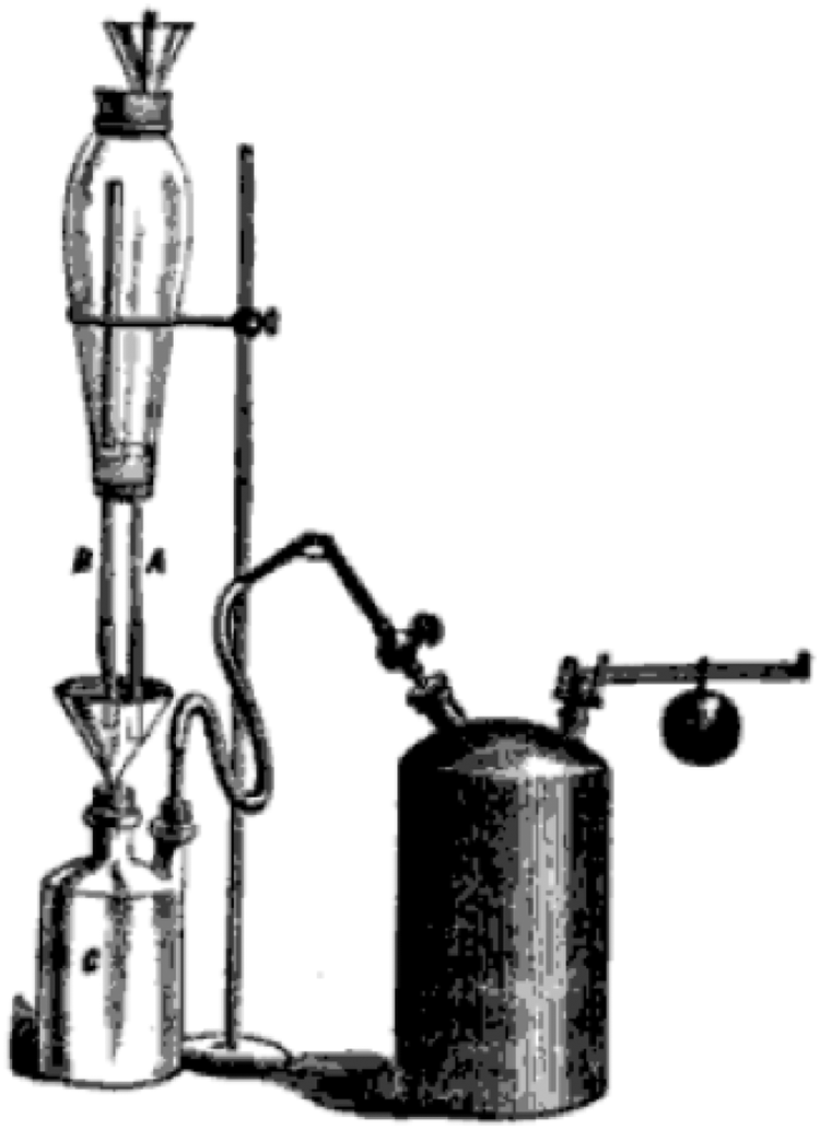
The filter washer described by Stevens ¹ in 1875 used a lamp chimney filled with water and closed at both ends to drip rinse water over a filtrate. The canister at the right of the device is a steam trap that was used to create a vacuum. (Illustration courtesy of Google Books)

This concept was expanded by Mitchell ² for a device with a very small aperture that could wash a piece of filter paper overnight. An additional refinement came from Elbert Lathrop ³ in 1917 to create a precipitate washer. He extended the air-admission capillary tube down into the funnel containing filter paper and a precipitate. When the funnel was full of liquid, the end of the capillary was submerged so that no air could enter. As the filter drained, the end was exposed to the atmosphere, air could enter the liquid reservoir, and the wash liquid dripped out until the end of the capillary was once again sealed off. ³

Some chemists included siphons in the washing apparatus. In 1893, Pickel ⁴ arranged a system of miniature siphons so that the flow of wash liquid agitated the sample, thereby exposing more surface area and improving the wash process. But unlike the earlier version of these devices, Pickel’s was ganged into a group of 10 individual washers. ⁴

There is only one mention in the literature of a chemist who dispensed with the siphons and drips in favor of a mechanical pump. W. D. Horne was working in commercial fertilizer analysis. Two grams of sample was placed on filter paper and washed with 10-mL aliquots of water until a total volume of 2500 mL was collected. To save time by washing automatically, Horne used a mechanical liquid dispenser designed to admit measured amounts of water directed so that the sample was agitated and the soluble materials leached out. Once started, no additional attention was needed. ⁵

Systems of siphons and solvent reservoirs were also used for intermediate infusion extractors. Unlike continuous extraction, these devices first allow one lot of solvent to come in contact with the sample, then remove it, and substitute another lot. Writing in 1922, Sir Thomas Edward Thorpe noted that the use of siphons in intermediate infusion liquid extractors for automated operation dates back to 1879. By 1922, there were more than 200 versions described in the chemical literature. Thorpe said that may of them were “triumphs of glass-blowing, but promise to be very fragile and difficult to clean.” ⁶

The same could be said for most of the systems described here, but this did not stop chemists from designing automatic burettes and pipettes that used systems of siphons to control liquid levels. Squibb ⁷ in 1894 created an “automatic zero burette.” An inverted siphon inside the burette controlled the zero point, but it could be adjusted for liquids of different viscosities. The burette was designed for busy labs that had repeated titrations using the same solutions. That same year, Greiner ⁸ developed an automatic pipette for use in the Babcock milk test. The concept was similar to the automatic burette as a siphon in the glass midsection controlled the liquid level. ⁸

The use of siphons for the addition of a washing or percolating reagent continued well into the 1920s and 1930s. Hibbard ⁹ at the UC Berkeley College of Agriculture wrote that although these types of devices were convenient, they tended to operate too quickly for percolating soil samples. Hibbard’s goal was to extract 20-gram soil samples over periods ranging from 15 to 30 h. His solution was to incorporate a “regulating train” between the 20-liter solvent reservoirs and the sample container. The regulating train was a series of three smaller reservoirs each fitted with two siphons. As one reservoir in the train filled via an entrance siphon, the exit siphon delivered the solvent to the next reservoir at a fixed rate. Adjusting the heights of the siphons in the smaller reservoirs controlled the flow rate. The final flow out of the apparatus was about 40 drops per minute, and even this was too high. A flow splitter divided the solvent flow so that only half actually percolated the sample. The other 50% could be diverted to another sample or collected for reuse. ⁹ Siphons, overflows, and reservoirs continued to be the basis of many automated devices during the 1930s.^10–14 In addition, several stills were invented that used float valves to control the rate of water addition to the pot flask or the supply of electricity to the heating element. Most of these were constructed by chemists and were not offered by equipment manufactures.^15–17

During the 1920s, we also see specialized devices used for solvent extractions in botanical research. Palkin et al. ¹⁸ in 1925 created continuous liquid-liquid extractors with internal diffusers so that the extraction solvent would be “sprayed” through the aqueous phase. The increased surface area improved extraction efficiency, and the entire apparatus replaced manually shaken separatory funnels.

Two years later, Palkin appears again in the literature as the coinventor of two new extraction devices. ¹⁹ The problem they sought to address was that dripping or percolating solvent through a powered botanical sample by gravity tended to compact it. By introducing the solvent stream from below the sample, it was kept in suspension. A slightly more complex version of the same apparatus used a stream of solvent vapor to provide additional stirring. ¹⁹

While laboratory scientists were tinkering with glass, the coal and power generation industries were embracing automation. The earliest device specifically manufactured and sold as a piece of laboratory automation was a grinder designed to prepare coal samples. Buying coal “by analysis” was a new idea in the early 1900s as large coal consumers such as power companies and industrial plants demanded to know more about the quality of the materials they were buying. The federal government began a system where supply contracts were based on the heating value of the coal. Although the actual coal analysis was well developed, obtaining a representative sample was both time-consuming and prone to error. A large sample had to be crushed, divided, and crushed again until a small, uniform, and representative sample was obtained. The procedure was prone to error, and a great many nonrepresentative samples found their way into laboratories. The Sturtevant Automatic Coal Crusher ( Fig. 2 ) was designed to solve this problem. Pieces of coal, 3 inches or smaller, were fed into a hopper on top of the machines and passed through “crushing members” of gradually decreasing size until they were out through a discharge chute. A separate sampling chute was arranged so that a fixed percentage of the crushed product could be collected separately. The entire apparatus was powered from an external motor. ²⁰

Figure 2.

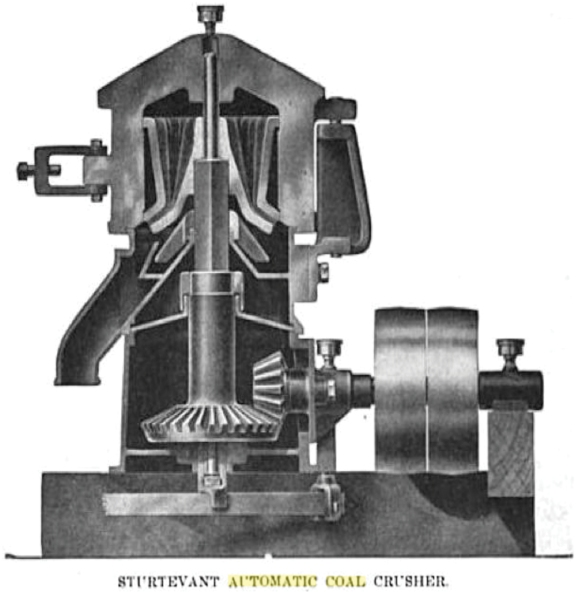
The Sturtevant Automatic Coal Crusher could reduce large pieces of coal to a size more suited for laboratory analysis and partition out a representative sample. This greatly improved the efficiency of coal analysis. (Illustration courtesy Google Books)

In the 1900s and early 1910s, a number of systems were used for measuring carbon dioxide in flue gasses as an aid to optimizing combustion control. This measurement was often achieved by passing a sample of the gas through a sodium hydroxide solution where it would be absorbed and thus change the pressure of the system. A manometer connected to the sample chamber was calibrated to record the percentage of CO₂ in the gas stream. An early commercial system was sold by Simmance-Abady. A system of weights and counterweights operated a set of valves that filled a closed tank with water. As the water rushed into the tank, it drew a sample of flue gas along with it. Once the tank was full, the water pressed the gas against the lid. The gasses were allowed to escape through a small tube and passed through a smaller tank filled with potassium hydroxide solution to scrub out the CO₂. The pressure of the gasses minus the CO₂ was read from a gauge. There was a provision to attach the gauge to some sort of recorder, but how this was done is not recorded in the literature. At the end of the measurement, the tank was emptied, pulling the remaining gas out of the system, and the whole process was repeated. The apparatus was capable of extended periods of unattended operation but only provided intermittent readings. ²¹ A continuous system was sold as the Autolysator ( Fig. 3 ) by Stache, Johoda, and Genzken. ²¹

Figure 3.

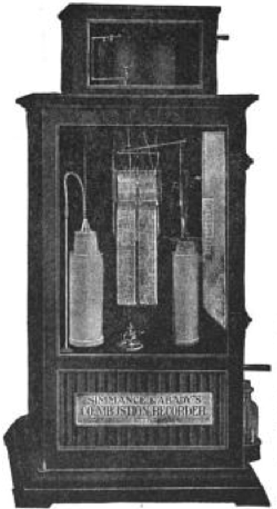
The Autolysator was one of the first automated analysis instruments ever sold commercially. This 1912 model used a complex system of clockwork, counterweights, and a chart recorder to provide real-time measurements of carbon dioxide in flue gas. (Illustration courtesy Google Books)

Although chemists seemed content to develop new methods of measuring carbon dioxide in flue gasses, electrical power engineers William Booth and John Kershaw took a more jaundiced view in a paper read before the Institution of Electrical Engineers in 1905. Their argument was that theoretically, such devices could improve combustion efficiency by monitoring CO₂, but in practice they required careful operation and proper maintenance if they were going to generate data of any lasting value. They were quite blunt on that point:

Automatic apparatus of all kinds is, we admit, of great service, but not in the direction properly supposed. It enables on skilled and efficient man greatly to increase the number and extent of his duties, and practically to treble of quadruple his efficiency; but it does not, and cannot, give accurate and valuable records when placed in the hands of untrained men. ²²

Although these combustion analyzers are not truly examples of laboratory automation, they were highly significant to the development of the field. During the ensuing decades, there was an overlap of process control automation and laboratory automation. Real-time scientific control of production processes opened the doors for automation in the laboratory, although the pathway was far from smooth.

Taylor and Hugh, ²³ working at DuPont, observed that American process industries were slow and reluctant to adapt automated process controls, preferring to devote their energies to rapid analytical techniques that could be performed by their internal quality control laboratories. Noting that gas analysis seemed a promising area for automated control, because handling gas samples in the laboratory was more difficult than liquid or solid samples, they developed a system where carbon dioxide gas was bubbled through a closed vessel and changed the electrical conductivity of a solution.

Solution conductivity measured with a Wheatstone bridge and a conductivity sensor was used to control the sulfuric acid content of a paper manufacturing wash bath. When the solution conductivity changed, a set of relays opened valves to allow more acid into the bath. The inventor was an electrical engineer named Philip E. Edelman of New York City. At the time, acid content of baths was regulated manually in a tedious process, but Edelman claimed his device could eliminate human error. ²⁴

Electronics Appear, 1920–1940

Taylor, Hugh, and Edelman were in the vanguard of a new era in laboratory automation when electronics were increasingly important. Initially, the most important automated instruments used conductivity measurements made with a Wheatstone bridge.

During the First World War, a need for rapid gas analysis prompted researchers at the University of Birmingham, England, to use thermal conductivity as the basis of gas analysis. Similar in concept to a thermal conductivity detector (TCD) on a gas chromatograph, the device measured the conductivity changes in a heated wire under a stream of gas. As the composition of the gas changed, the heat capacity of the gas changed, and therefore the wire’s conductivity also changed. Unlike the TCD, there was no chromatographic separation of the gas mixture prior to analysis. Despite this limitation, commercial versions of the device were introduced by the Sperry Gyroscope Company and the Cambridge Instrument Company. A great advantage, however, was the ability to provide automated operation in remote locations. ²⁵

Weaver and Palmer ²⁶ in 1920 noted that of the common gas analysis methods—density balances, interferometers, direct weighing, and chemical separation followed by analysis—thermal conductivity had the best sensitivity, required the least operator skill, and required smaller sample sizes. However, the system did require calibration with an external standard and was more expensive. ²⁶

Commercial pH electrodes were not available until the mid-1930s, and their absence was keenly felt in the sugar refining industry. Sugar refining is a multistep process that requires precise pH control at several points. One of the steps involves adding lime to precipitate the nonsugars. An early test of automatic control for liming cane juice in sugar refining was made in 1928 at a Puerto Rican sugar refinery. The equipment used in the test included a recording potentiometer, a tungsten-calomel electrode, temperature compensation, and powdered lime dispenser. However, a poor understanding of the limejuice reactions hampered full implementation, as it was not understood how much lime should be added in response to a particular electrode signal. ²⁷

Once the impurities have been removed from the juice, the remaining calcium is precipitated out in a carbonation step. Balch and Keane ²⁸ in 1928 once again used a tungsten-calomel electrode to measure electromotive force (EMF), whose value was related to but not an actual measure of the pH in sugar beet refining. Two carbonation steps are required to precipitate the remaining lime. Timing these steps was critical with the optimal results obtained after the calcium carbonate from the first step had completely settled out of solution. A titration was usually used to determine this point, but a reliable pH electrode would have greatly simplified the task and opened it to automation. The electrodes available at the time were too slow to equilibrate, too complex for use on the factory floor, or too prone to poisoning by the sulfur dioxide used in a later step. Balch and Keane, working in the federal government’s Bureau of Chemistry, somewhat optimistically asserted that the tungsten-calomel electrode, working in conjunction with a chart recorder, could be used to control the addition of these gasses automatically.

A year later, in 1929, Holven ²⁹ would explore the limitations of the tungsten and calomel half cell for the following reasons: There was variability in calibration, the electrode could not be readily interchanged once installed, the electrodes did not last very long, and they were prone to poisoning. Holven concluded that until a more reliable electrode was available, automated pH control would have to wait. In the absence of reliable electrodes, most sugar producers used pH indicators.

Automation was more successful in the rubber industry. Among the more challenging tasks was the accurate plotting of tensile strength in units of kg/cm² against percent elongation. These stress and strain data were necessary for rubber compounders to understand how a material performed.

The manual methods for stress and strain were imprecise at low elongations and, when done manually, suffered from the delays between the verbal call to record data and the actual reading of the strain gauge. Two operators would attach one end of a sample to a load gauge and begin to stretch the rubber. One operator, holding a ruler, would measure the distance between marked points on the piece, whereas the other would read the gauge at the call of the first. The automated method, first reported in 1930, was used to test the rubbers used in tire treads. It used a 15.2-cm circumference rubber ring stretched over four pulleys. The data were recorded by an “autographic” method. A plotting device burned a hole in the recording paper each time the rubber’s length doubled. The new device required only one operator and produced more accurate results. ³⁰

Other automated rubber testing devices were used to measure hardness and, by eliminating the need for an operator judgment, improved the testing methodology. ³¹

In 1929, the first of two significant automated titrators was introduced; one was built by chemists at New York University and the other by chemists at Eastman Kodak. Both used a photocell to sense the color change to an indicator at a titration’s end point. The introduction of the instrument by New York University excited comment outside of the analytical chemistry community. The New York Times reported on a device created by Dr. H. M. Partridge and Professor Ralph H. Muller of the Department of Chemistry at New York University. The instrument was demonstrated at a meeting of the New York Electrical Society in December 1929. At the start of the analysis, a relay opened the burette, and the titrant was allowed to drip into a glass vessel where the reaction occurred. When the end point was reached, the photocell detected the color change and activated another relay to close the burette. A radio tube was used as the signal amplifier, and the inventors claimed that the device was 165 times more sensitive to color differences than the human eye. For public demonstrations, an alkali was titrated with an acid. Phenolphthalein was used as the indicator so the end point was indicated by a change from red to colorless. Partridge and Muller stated that the device would work equally well with the titrant and sample reversed; it was merely a question of adjusting the sensitivity of the photocell. ³²

Popular Science Monthly reported on the device in March 1930 and commented on its ability to save time in the laboratory and provide more accurate analysis than a human. The magazine also reported that when the end point was reached, a red light turned on and a bell was rung, details the more staid New York Times did not mention. ³³ Muller would later write a highly influential column on instrumentation for Analytical Chemistry and was well respected for his many insights into the development of the field. ³⁴

The titrator built a few years later by K. Hickman and C. R. Sanford at Eastman Kodak in Rochester, New York, was more sophisticated. It was designed for acid-base titrations and intended for use in paper-making operations. The sample was drawn from a tap connected to an alum bath or to a wash bath. It flowed into a receiving flask. On one side of the receiver, there was a siphon into the titration vessel, and on the other side, there was a column of mercury. As the receiver filled, the mercury rose, closed two electrical contacts, and activated a set of valves that emptied the previous sample from the titration vessel. Meanwhile, the fresh sample rose through the siphon and was eventually flowed down into the titration vessel. As it passed down the siphon tube, it sucked a small amount of indicator from another reservoir. The titrant valve was opened, the end point was detected by the photocell, and the results of the titration were plotted on a chart recorder. ³⁵

One of the first American Chemical Society meeting sessions devoted to process automation was held in 1922. In 1929, Ismar Ginsberg would assert that although the chemical manufacturer could not avoid the use of thermometers, pressure, humidity, and other measurements, the use of the these devices had not generally been optimized. Using instrumentation for process control was only beginning to become common, and not all companies fully appreciated the need to integrate instrumentation readings with what was known about the underlying chemistry of their processes. ³⁶ Only 8 years later, Charles Allen Thomas could confidently assert that “supplanting automatic instrumentation for the personal equation results in a smoother, steadier operation and greater yield of a more uniform product with a reduction in cost.” ³⁷ Some examples of the industrial applications where automated controls were already common included temperature and steam pressure regulation in silk production, water flow in natural gas condensers and cracking units, petroleum refining, heat-treating ovens, coke ovens, and steel production. Allen drew some additional examples from the chemical industry, including the reaction vessels where nitrification, sulfonation, and reduction reactions were carried out. A manufacturer of resin-impregnated fabrics was able to recover 98% of the acetone used in the process through the use of an automated unit whose single operator, it was claimed, never touched the controls between starting it in the morning and turning it off at night. It was also asserted that the cost of labor in the European chemical industries was lower, and as a result, automated control technologies lagged behind those in the United States but that producers in England and Germany were increasingly developing this technology. ³⁷

Siphons, overflows, and reservoirs continued to be the basis of many automated devices during the 1930s.^10–14 In addition, several stills were invented that used float valves to control the rate of water addition to the pot flask. Most of these were constructed by chemists and were not offered by equipment manufactures.^15–17

Rosie the Robot: The Second World War

The United States began increasing its industrial production to meet the demands of the Second World War in the spring of 1940. By the end of 1941, the civilian labor force numbered 56 000 000, and 1 500 000 persons were serving in the armed forces. In heavy industries, 5 600 000 workers, or about half the total, were employed in defense-related projects. Defense spending reached $75 000 000 per day, and overall industrial production was up 66% from its 1935–1939 average. ³⁸ In 1942, the United States produced 47 000 aircraft, and the total would rise to 100 000 aircraft in 1944. By 1944, the civilian labor force rose to 64 010 000 persons, and 10 000 000 were serving in the armed forces. The demand for all kinds of war materials also increased the demand for chemists and chemical technicians. This demand was largely met by increasing the size of the labor force through the recruitment of women. The U.S. Army even developed a specialized training program in general chemistry. Laboratory automation would not be widely seen as a viable means of increasing laboratory productivity until after the war.

That did not stop scientists from developing dedicated devices for specific tasks. Some of these were intended to allow unskilled persons to perform complex tasks such as titrations, others were used to stretch the manpower available in the laboratory such semi-automated stills used in petroleum analysis, and still others were designed to conserve strategic materials such as rubber, copper, and other metals. An all-glass constant-rate reagent addition device was constructed at Princeton University ( Fig. 4 ). It had no moving parts and used no rationed materials. It consisted of a U-shaped glass tube filled with the reagent that would be dispensed. In one arm of the tube, a distillate was collected at a constant rate. The distillate was chosen to be heavier than the reagent and so it sank, thereby raising the level of the reagent. On the other arm, a take-off tube drained the reagent into the reaction vessel at a rate equal to that of the distillation. ³⁸

Figure 4.

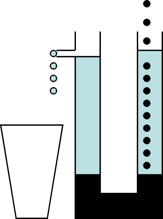
Constructed during the Second World War and designed to have no moving parts or use any rationed materials, this constant-rate reagent addition device was used at Princeton University. A heavy distillate (dark color) collected in the U-shaped tube displaced the reagent (light color) at a rate equal to the distillation rate. (Author’s illustration)

An example of the type of automation to conserve manpower was the semi-automated still developed by Bassett Ferguson Jr. of the Ugite Sales Corporation of Chester, Pennsylvania, for petroleum analysis. The still was operated at a constant rate and employed automatic temperature recording. In the take-off collector was a glass stopper containing an iron core. Every 30 seconds, an electromagnet activated and pulled the stopper out, allowing the contents to drain into a collection vessel. Knowing what sample was collected at any one point on the distillation temperature curve allowed the fraction to be identified. ³⁹ Ferguson also developed an automated pressure regulator that employed a manometer whose column of mercury flowed over contacts opening and closing the control circuits. This type of control arrangement had long been employed, but Ferguson added glass bulbs at the top of the manometer columns. Pressure in the bulb connected to the gas system either pushed up on a relay (sending a signal to lower the pressure) or allowed a column of mercury that spanned two electrical contacts to rise (sending a signal to raise the pressure). ⁴⁰

The mercaptan automatic titrator for gasoline developed by the Shell Oil Company was an example of the type of device designed specifically to alleviate a skilled labor shortage. In 1941, chemists working at Shell developed a potentiometric titration procedure, ⁴¹ and by 1943, the procedure was automated. ³⁸ The entire device was designed for use by an unskilled operator who would load the sample, add a conductive media, press the start button, and read the result directly from the chart recorder. In mercaptan titrations, the end point was determined by an electronic potential that was unique for a particular type of gasoline. Therefore, the end point had to be preset according to criteria that would, presumably, be determined by more skilled personnel. This titrator had a clock motor driving a cam that activated a switch that, in turn, opened and closed the burette valve. This operated in conjunction with an iron core inside the burette that was moved by an electromagnet to dispense the titrant. The apparatus did not track the volume of the titrant that was being added; instead, it recorded the total volume in the titration cell by using a chart recorder. In any manual titration, a skilled operator could vary the rate of titrant addition as the end point approached; the electronics that would automate this would not be available for another decade. Thus, the rate of titrant addition was a compromise between speed and accuracy.

The most sophisticated laboratory automation created during the war was used to control amperage during electrodeposition analysis. Two metals can be separated with a constant current if one of them is above hydrogen in the electromotive series and the other is below hydrogen because once the lower metal is deposited, hydrogen gas is generated in preference to the upper metal. The only requirement of the operator is that the current periodically has to be adjusted to compensate for the loss of electrolytes. However, when the metals are close in the series, the amperage control has to be precisely and tediously controlled. An automated system that could separate copper from a hydrochloric acid solution was developed. In this automated system, the voltage increased as the reference cell and the cathode increased as the copper was deposited. The electrolyzing current needed to be decreased in response so that the potential remained constant. A voltmeter signal was fed to an amplifier-relay circuit that activated an electric motor. The motor was connected by a set of gears to a Variac that controlled the potential. The device was limited to a total applied EMF of 10 volts and could not correct for a positive drift in the cathode potential. ³⁸

James Lingane of Harvard University later introduced a version of the device that eliminated these problems. An ammeter read the electrolyzing current and controlled a second current in opposition to the cathode-reference electrode EMF. By detecting an imbalance between the cathode- reference electrode EMF and the opposing current, the control circuit was triggered and drove the Variac. ³⁸

During the war years, there were still many simple automated devices designed to make life easier in the laboratory. A shortage of pure reagents forced many laboratories to perform their own purifications by distillation, but there was also a shortage of skilled technicians needed to operate stills. This prompted a new set of automated and semi-automated stills using intermittent siphons and float valves. In a still operated by the Louisiana State Department of Health, the rate of distillation was controlled by a collection flask placed on the end of an equal-arm balance ( Fig. 5 ). On the other arm was a graduated cylinder of water and two electrical contacts dipping into a pool of mercury. Water was allowed to drip into the graduated cylinder at a controlled rate. When the contacts were in the mercury, a circuit powering the heater was closed. As long as the collection flask filled no faster than the cylinder, the arm remained balanced and the circuit remained closed. If the rate of distillation exceeded the rate at which the cylinder filled, one balance arm dropped, the opposite arm rose, the contacts were withdrawn from the mercury, and the power was turned off. Although this seemed like a very crude device, it was actually capable of controlling steam distillation rates to within 1 or 2 mL per hour. ³⁸

Figure 5.

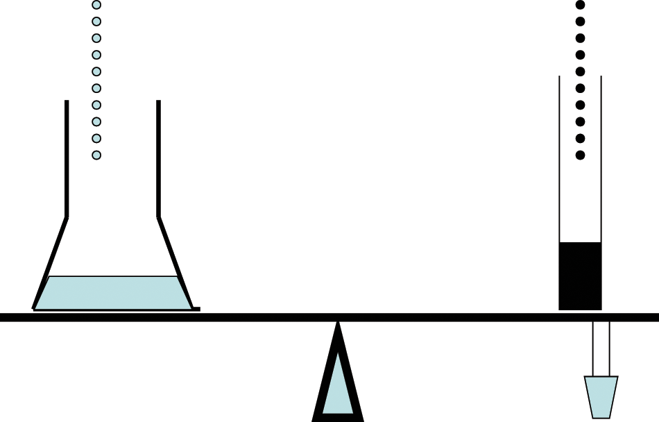
A counterweighted balance arm that was connected to mercury contacts opened and closed as the arm moved and controlled the rate of distillation in this still operated by the Louisiana Department of Health. (Author’s illustration)

The timing siphon occupies a curious place in the history of automation, linking the eras when automation was dominated by the glass blower and the tinkerer with the era dominated by electronics. It allowed an apparatus to be turned on and off at regular intervals. The timing siphon was a product of wartime necessity and consisted of electrical contacts placed in a large tube. The tube filled with water and the contacts closed. As a siphon connected to the tube filled, it began to empty the tube and the contacts opened. The depth of the contacts could be adjusted for different on/off cycles. If the liquid in the device did not conduct electricity, the same timing effects could be achieved with photocells. ³⁸

Laboratory Automation Goes Mainstream: The 1950s and 1960s

By the end of the Second World War, the use of automatic control equipment in chemical manufacturing had become routine, and there was a new need for trained instrumentation experts. In response to this demand, the chemical engineering department at Washington University incorporated experiments where students learned the operating characteristics of temperature-controlled equipment. ⁴²

In the 1950s, the number of new devices that used siphons, floats, and reservoirs that drip dropped off dramatically. What examples that do appear in the literature were being used to control fraction collectors for chromatography or distillation. Turntables were advanced in response to photocells, mercury switches, or capacitance. ⁴³ Mader and Mader ⁴³ in 1953 placed a glass reservoir and siphon assembly on a rocking arm so that as the reservoir filled, the arm rocked, a mercury switch activated, and the turntable advanced as the siphon drained the reservoir into an Erlenmeyer flask. Van Duuren ⁴⁴ in 1960 used electronic control to open the siphon valves in response to a timer, noting that a problem with paper chromatography was the time necessary to allow an equilibration time for the paper and a solvent placed in a tank. Once the equilibration was complete, the developing solvent was added and the chromatography began. Adding a timer to the developing solution addition equipment meant that an operator could set up the tank, set the equilibration time, and walk away and would not have to return to add the developing solution. Martin ⁴⁵ in 1958 created another timer-chromatography combination, noting that chromatography runs were getting longer. His device opened a valve, allowing solvent to flow into the system at a preset time. It was now possible for a chemist to automatically start a chromatography run on Sunday and have the results on Monday morning.

The laboratories of the Socony-Vacuum Oil Company combined older automation ideas, conductivity, and paper tapes to create a device that automatically determined the sediment and moisture in their oil pipelines. A small sample was removed from the pipeline and passed through a piece of moving filter paper. The sediment left a trace on the paper that could be quantitated by comparison with standards. The electrical conductivity of the paper changed with the moisture content and could be permanently marked by a series of holes punched in the tape. ⁴⁶

For the laboratory chemist who wanted automation but did not want to tinker with motors, chart recorders, timers, or elaborate glassblowing, there was a plethora of new automated titrators. By 1948, about nine automatic potentiometric titrators had been described in the literature. A new type of titrator designed in 1948 used a syringe attached to a motor to add the titrant. Unlike a burette that dripped, the motor speed could be varied for different types of titrations. This device was seen as being superior because it used a recording potentiometer to plot the titration curve. The potentiometer could also be set to stop the titrant addition at a preset point. ⁴⁷

Automated Karl Fischer titration was announced in 1952 by chemists working at Merck in Rahway, New Jersey. By this time, there was already a large volume of literature about this technique and commercial titrators were available, but this automated system sought to address the difficulty of determining the end point. The usual end point was from canary yellow to light amber, and although easy to distinguish in colorless solutions, colored samples or suspended solids were difficult to titrate. Potentiometric end-point detection was tried, but the Karl Fischer titration had to be done under anhydrous conditions that precluded the use of reference electrodes, salt bridges, and other electrochemical components. The “dead stop” technique used a polarization end point where an increase in the current between two platinum electrodes corresponded with a depolarization of the electrodes found at the titration’s end point. The developers of the titrator at Merck boasted that automatic reagent addition was used and that there were no vacuum tubes. ⁴⁸

Another significant step forward was the creation of automated coulometric Karl Fischer titration that regenerated Karl Fischer reagent from the iodine present in a solution of depleted reagent. The use of such a technique was not new, but the chemists at the Oak Ridge National Laboratory in Oak Ridge, Tennessee, used a modified Leeds & Northrup pH indicator to control the titration. Commercial pH meters were increasingly used to create automated devices, especially using millivolt or polarization end points. The Leeds & Northrop meter was able to provide a polarizing current and was fitted with a cutoff circuit. ⁴⁹

J. P. Phillips of the University of Louisville published a book on automatic titration technology that reviewed all automatic and semi-automatic titrators that had been described in the literature or were available commercially as of 1958. Discussions of photometric, amperometric, conductometric, thermometric, and potentiometric devices were described in the book with a separate chapter devoted to coulometric titrations. Commercial devices such as the Beckman Model KF-2 Aquameter were included. A comment in the preface of the book, however, provides some illumination on how chemists viewed automation at this time. Titration, it was said, is the “only modern instrumental method of analysis” in which a knowledge of chemistry was more important than knowledge of electronics or physics. Clearly, the ideal of a system being user-friendly was still some years off. ⁵⁰

During the first half of the 1950s, regular reviews of automation technologies were appearing in the literature. By this time, there was less of an emphasis on design and “manipulative details.” There were more commercial instruments available and even competition between manufacturers. The literature was also filled with examples of user experience. Semi-automated devices for research use were now more fully automated for use in routine quality control. ⁵¹ A journal devoted to instrumentation, the Instrument Engineer, appeared in 1952.

By 1960, the Beckman Model B, Beckman DU, and Cary spectrophotometers were modified to allow titration cells to be placed in their sample compartments. A solenoid-operated burette valve could be triggered by the photometric end point, whereas others used recording devices capable of generating first, second, and even third derivative plots so that the operator had a choice of end point determination. ⁵²

The first mention of a computer for use in conjunction with automation was in 1948. The Reeves Instrument Corporation introduced “an office-size electronic computer.” It was an analog computer using circuits to model differential equations, and for the first time, chemical researchers and persons designing automatic process control equipment could create electronic simulations of their processes. ⁵³ The first mention of a digital computer for laboratory instrumentation came in 1952 when the Atlantic Refining Company announced that it had developed a mass spectrometer and digital computer combination capable of performing a “complete molecular analysis of a 20-component hydrocarbon mixture in 10 minutes and type out the results on a paper tape.” The input to the computer came through an analog to digital converter, referred to as a “selector” that was developed by Consolidated Engineering Corporation. ⁵⁴

The first truly automated systems where samples were loaded at one end and multiple analytical results came out the other appeared in medical laboratories during the mid-1950s. During the first International Congress on Clinical Chemistry held in New York City in September 1956, physicians and clinical chemists were introduced to an automated blood analyzer manufactured by Technicon and originally developed the Pathology Department of Western Reserve University School of Medicine. The Technicon analyzer took a small sample of blood and within 2.5 min measured the levels of urea, sugar, and calcium. ⁵⁵

The Technicon machine worked by pumping the blood sample through a chamber where the analytes were separated from the sample by a cellophane membrane. Color-sensitive reagents were then pumped into a sample cell and the concentrations were determined by the intensity of the color change and read by photocells. ⁵⁶ Interest in automated systems for clinical laboratory work would grow during the 1960s. Although several instrument manufacturers expressed reluctance to enter this market, by 1963 it was predicted that the market for clinical laboratory instruments would grow 20% annually for the next 5 years. Chemical and Engineering News reported that a growing number of companies were either entering or closely studying this market and that hundreds of thousands of dollars were already invested in developing clinical laboratory robotics. ⁵⁷ In 1970, the National Institutes of Health and the Atomic Energy Commission announced that they had licensed five companies to manufacture automated laboratory automation that used technologies developed at the Oak Ridge National Laboratory. The systems developed at Oak Ridge were spectroscopic and used both light absorption and transmittance. ⁵⁸

Another significant analysis system adopted during the 1950s was created by the New York Central Railroad and used for lube oil analysis. In a program implemented at the personal instigation of the railroad’s president, a Baird-Atomic Direct Reader for oil analysis was installed at the company’s Cleveland Technical Center in the late 1950s. Lube oil analysis consists of heating a sample of used lubricating oil and measuring the emission spectra of the metals it contains. As engine parts wear out, small metal particles become entrapped in the oil. Knowing which metals are in the oil can predict which parts may fail or identify parts in need of replacement. ⁵⁹

In the years after the Second World War, the railroads replaced steam locomotives with modern diesels. After years of deferred maintenance during the Great Depression, the new streamlined locomotives were powerful symbols of the railroads’ commitment to new technology and faster service. Aside from any practical value of the oil analysis, the success of the program provided tremendous public relations value for both the railroad industry and automated chemical technology.

The New York Central Railroad became the leader in diesel engine lube oil analysis and had laboratories established throughout the system for that purpose. The Cleveland Technical Center eventually began performing lube oil analysis for other industries. Marketing the service under the name “Spectra-Check,” the client list would include Trans World Airlines and the U.S. Navy. The service later became CTC Analytical Services. ⁵⁹

The Power of the Transistor and a Glimpse of the Internet

During the 1950s, the one electronic technology that truly promised to revolutionize the laboratory was the transistor. When used in conjunction with a system of fast-responding sensors, it would allow for the collection of thousands of data points. Developed at the height of the cold war, few of these devices were available to civilian scientists, but their arrival was eagerly anticipated. ³¹

The other development that excited the imagination of scientists was the “information appliance.” This was the computer that would not simulate instrumentation readings or decode mass spectrometer results but automate the tedious and time-consuming task of searching the scientific literature. It was not entirely clear if the appliance would be somehow networked or have local storage for the documents. The user, however, would look up the references in some sort of bound directory similar to a telephone book. Automated searching by keyword was still not envisioned. Once the desired paper was found, the scientist would be able to dial its number and it would appear on a screen. ³¹

One of the first multifunctioning, programmable, computer-controlled robots for laboratory use was introduced by a Syracuse University analytical chemistry professor, Daniel J. Macero, and a graduate student, Brian J. McGrattan. At the 1984 Eastern Analytical Symposium, they demonstrated a computer-controlled, reprogrammable robotic arm that could pick up and move labware. This robot, and others like it, marked the moment when laboratory robotics was freed from specific instruments and specific tasks. ⁶⁰

Any automation project is a mix of need, enabling technology, and a creative mind-set. The definition of automation, however, is subject to change. Because the number and capabilities of the enabling technologies have been steadily increasing, what was cutting-edge automation for one generation is often regarded as being slow and cumbersome by the next generation. With few exceptions, laboratory automation and robotics were confined to specific tasks and largely created by the people performing those tasks. It was not until the 1950s that there was a sufficient mass of enabling technologies for instrument suppliers to enter this market in appreciable numbers.