
Abstract
Study Design:
Retrospective/prospective study.
Objective:
Models based on preoperative factors can predict patients’ outcome at 1-year follow-up. This study measures the performance of several machine learning (ML) models and compares the results with conventional methods.
Methods:
Inclusion criteria were patients who had lumbar disc herniation (LDH) surgery, identified in the Danish national registry for spine surgery. Initial training of models included 16 independent variables, including demographics and presurgical patient-reported measures. Patients were grouped by reaching minimal clinically important difference or not for EuroQol, Oswestry Disability Index, Visual Analog Scale (VAS) Leg, and VAS Back and by their ability to return to work at 1 year follow-up. Data were randomly split into training, validation, and test sets by 50%/35%/15%. Deep learning, decision trees, random forest, boosted trees, and support vector machines model were trained, and for comparison, multivariate adaptive regression splines (MARS) and logistic regression models were used. Model fit was evaluated by inspecting area under the curve curves and performance during validation.
Results:
Seven models were arrived at. Classification errors were within ±1% to 4% SD across validation folds. ML did not yield superior performance compared with conventional models. MARS and deep learning performed consistently well. Discrepancy was greatest among VAS Leg models.
Conclusions:
Five predictive ML and 2 conventional models were developed, predicting improvement for LDH patients at the 1-year follow-up. We demonstrate that it is possible to build an ensemble of models with little effort as a starting point for further model optimization and selection.
Keywords
Introduction
For the past decade, various advanced techniques in predictive analytics commonly known as machine learning (ML) have gained interest in orthopaedics and medicine at large. 1 The effectiveness of ML compared with more traditional methods has been well demonstrated in solving classification problems, especially in medical image analysis, but as of yet has not been widely adopted by spine surgeons.2,3 The increasing accumulation of health data leaves a gap between available data and actual data use. ML might leverage the use of large amounts of health data and accelerate the development of predictive, preventive, or personalized medicine. 4 However, the application of ML algorithms has traditionally required specific programming skills not readily available among medical professionals. The reliance on data scientists to explore health data may be an obstacle to widespread use of ML. The advent of modern visual code-free software platforms might put ML in the hands of surgeons. 5 The purpose of this study was to assess the feasibility of predicting outcomes following lumbar discectomy by comparing 5 ML methods using a modern visual data science software platform, RapidMiner Studio. 6 Results were compared with 2 conventional learning algorithms. To demonstrate differences and similarities, these various methods were applied to single-center retrospective registry data collected on patients following lumbar discectomy.
Methods
Patient Population and Data Source
Patients who had surgery for lumbar disc herniation (LDH) at a single center from 2010 to 2016 were identified in the Danish national registry for spine surgery (DaneSpine). Of 3216 patients identified, 1988 had complete baseline and 1-year follow-up patient-reported outcomes (PRO) data. In all, 20 patients had extreme body mass index (BMI) values (>80 kg/m2) likely because of erroneous data entry and were excluded. A total of 1968 patients were included in this study.
Study Variables
Two primary health outcome variables were chosen for assessment: EuroQol (EQ-5D) 7 and the Oswestry Disability Index (ODI). 8 In addition, back and leg pain on the Visual Analog Scale (VAS; 0-100) 9 and patients’ ability to return to work were included. In accordance with generally accepted practice when solving classification problems, outcome variables were binary coded as either success or nonsuccess. 10 With the exception of return to work, success was defined as achievement of minimal clinically important difference (MCID). MCID thresholds were arrived at using the anchor-based receiver operating characteristic curve (ROC) method. 11 For both EQ-5D and ODI, 1-year postoperative response to the Short Form-36 Health Transition Item (Item 2) that asks the question, “Compared to one year ago, how would you rate your health in general now?” 12 was used as the anchor. Possible answers are “much better,” “somewhat better,” “about the same,” or “somewhat worse” or “much worse.” Cutoff for success/nonsuccess was set between patients who responded “somewhat better” versus “about the same.” For VAS back and VAS leg pain, responses to the Global Assessment questions at 1 year postoperatively were used: “How is your back pain today compared with before the operation” and “How is your leg pain/sciatica today, compared with before the operation?” Responses were “completely gone,” “much better,” “somewhat better,” “unchanged,” or “worse.” Cutoff for success/nonsuccess was set between patients who responded “somewhat better” versus “unchanged.”
In determining MCID thresholds, sensitivity and specificity were valued equally, and cutoff points were estimated from the coordinates of the ROC curves using the sum-of-squares approach. The smallest sum of squares of 1-sensitivity and 1-specificity identifies the point closest to the top-left corner in the ROC diagram space. 13 A wide variety of preoperative factors were selected as possible predictors, including gender, age, smoking status, level of pain, walking distance, and health-related measures (Table 1).
Descriptive Statistics of Study Sample: Baseline Patient Characteristics.
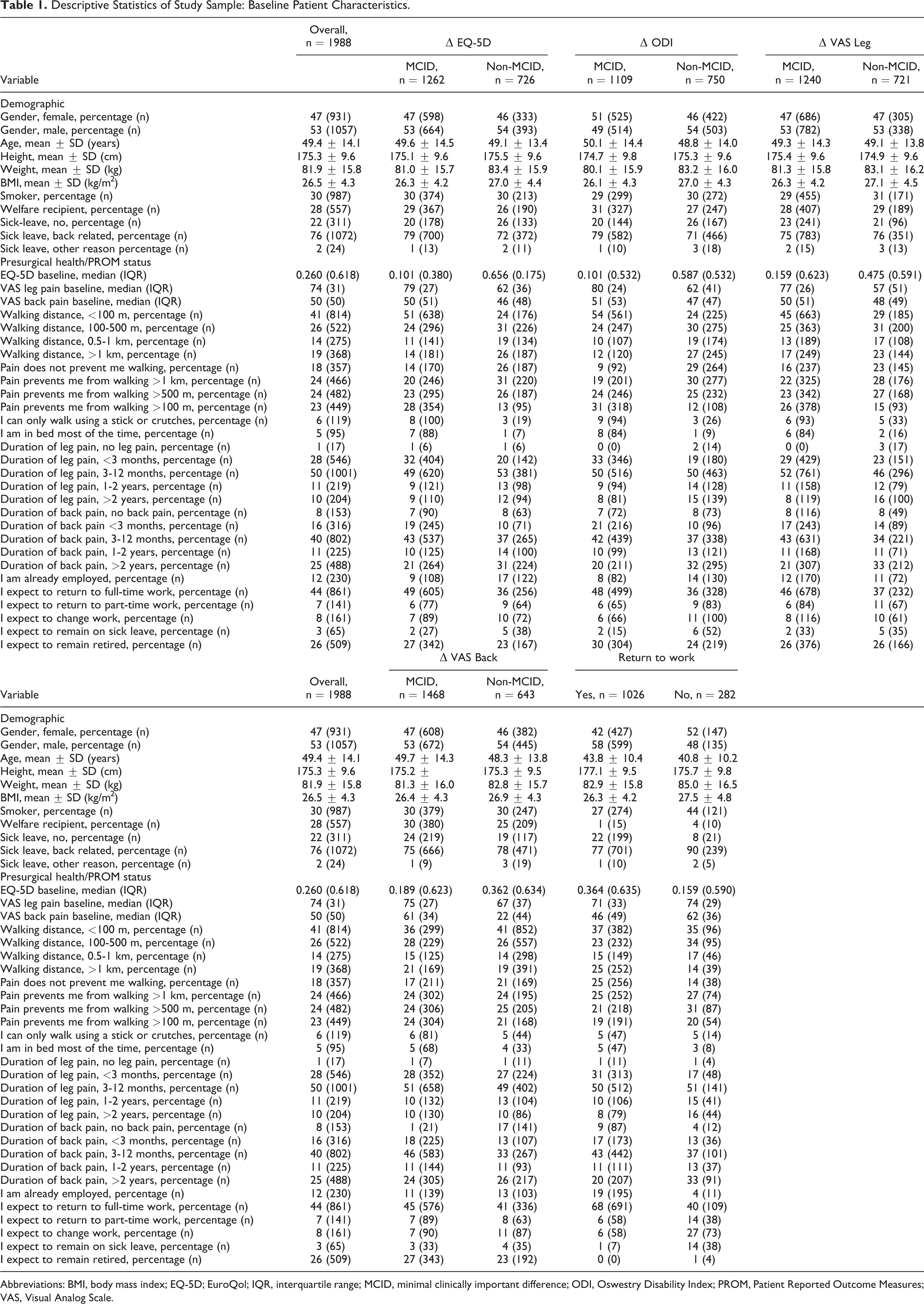
Abbreviations: BMI, body mass index; EQ-5D; EuroQol; IQR, interquartile range; MCID, minimal clinically important difference; ODI, Oswestry Disability Index; PROM, Patient Reported Outcome Measures; VAS, Visual Analog Scale.
Statistical Analysis and Data Handling
During data preparation, distance-based outlier detection was applied to identify and remove extreme cases, which were assumed to be erroneous data entries. 14 Less than 1% were identified as outliers and removed case wise from the data set. The resulting data were randomly split into a training, validation, and test set by a 50%/35%/15% ratio. Class imbalances ranging from 60% to 78%/40% to 22% were present in the target outcome measures. Many ML classification algorithms are sensitive to imbalanced data and have poor accuracy for the infrequent class. 15 To ensure optimal class performance of the models, synthetic minority oversampling was applied to the training and validation data sets. 16 The test set (holdout data) was left untouched. All data preparation was done in RapidMiner (Figure 1).
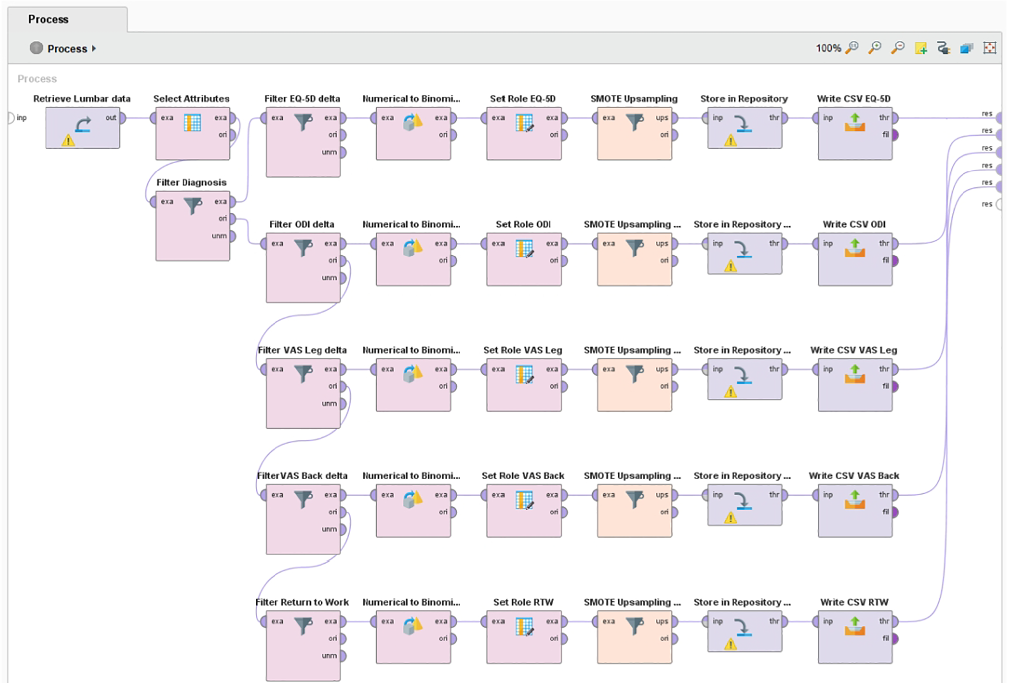
RapidMiner process for minority class upsampling of outcome measures using SMOTE.
For each outcome measure, 5 popular ML models were trained: deep learning, decision trees, random forest, boosted trees, and support vector machine (SVM). For comparison, 2 conventional types of models—logistic regression (LR) and multivariate adaptive regression splines (MARS)—were trained. With the exception of MARS, all modeling was performed in RapidMiner Studio 9.3.001 using the “Auto-model” feature. Further tuning was done adjusting model hyperparameters during validation. Auto-model does not support full cross-validation. Instead, performance is evaluated for 7 disjoint subsets of the validation data. The largest and the highest performance are removed, and the average of the remaining 5 performances are reported. MARS models were built and trained using R version 3.5.3 and the CRAN package earth.17,18 MARS models were tuned by manipulating model complexity (number of basic functions) and degree of interactions using the earth functions nk and degree. K-fold cross-validation was performed using the functions nfold (number of cross-validation folds) and ncross (number of cross-validations performed). In both software packages, model fit was evaluated during training by inspecting area under the curve (AUC) curves and the mean performance and SD of performance across validation folds. Final validation of all models was done by applying them to the test data set.
Machine Learning
In this study, ML is simply regarded as the study on how computers can learn to solve problems without being explicitly programmed. 19 More formally, ML can be stated as methods that can automatically detect patterns in data. The uncovered patterns are used to predict future data or other outcomes of interest. ML is typically divided into 2 main types: supervised and unsupervised learners. In the supervised approach, the algorithms learn from labeled example data. In the unsupervised approach, no corresponding output variables are presented. Algorithms are left to their own to discover patterns in the data. The ML methods used in this study are supervised. 20
Predictive Algorithms
LR is a highly popular method for solving classification problems and has been the de facto standard in many fields, including health care, for several decades. LR follows the same principles applied in general linear regression. However, because the outcome is binary, the mean of the regression must fall between 0 and 1. This is satisfied by using a logit model and assuming a binomial distribution.21,22
MARS is an advanced form of regression that extends the capabilities of standard linear regression by automatically modeling nonlinearities and interactions between variables. The MARS algorithm adapts to nonlinearities by piecewise fitting together smaller localized linear models that are defined pairwise.23,24
Deep learning belongs to a class of ML methods based on deep artificial neural networks (ANNs). An ANN is a simplistic representation of the functioning of a biological brain. The neural network consists of highly interconnected artificial neurons called nodes organized in several processing layers. Like synapses in a brain, the connections allow nodes to transmit signals to other nodes. Each node is initially assigned with a random numeric weight for each of its incoming connections. When a node receives signals from other nodes, the strength of the signals is adjusted by the associated weights. The resulting numbers are then summed and passed through a simple nonlinear function, which produces the output.25-27
Decision trees are models for classification and regression. A decision tree is structured like a flowchart resembling a tree. It learns by processing input from the top (root) and splitting data into increasingly smaller subsets following an if-then-else decision logic. Splits are made by decision nodes followed by another decision node or a leaf (prediction). Splits below nodes are called branches. The decision tree algorithm evaluates all possible splits in each step and multiple thresholds in order to make the most homogeneous subsets. 28
Random forest is an ensemble method where the training model consists of a multitude of ordinary decision trees. The final model is determined by majority vote when solving classification problems and mean value when tasked with regression. The basic idea is that merged together, the predictions of several trees should be closer to the true value than any single tree.29,30
Boosted trees are ensembles of very simple decision trees referred to as weak learners. The model is trained by gradually improving estimations by applying trees in a sequence, where each new tree is optimized for predicting the residuals (errors) of the preceding tree. Optimization is done by an algorithm that favors incorrectly classified predictions by assigning them a higher weight, which forces subsequent trees to adapt to the examples that were incorrectly classified by the previous trees. The idea is that many simple models when combined perform better than 1 complex model. 31
SVMs are commonly used to classify a data set into 2 classes. It achieves this by finding the line that best separates data points. Support vectors are the data points closest to the dividing line. When a data set is nonlinearly separable, SVM transforms data into a 3D dimension. The dividing line now resembles a plane. Data will be mapped into increasingly higher dimensions until a plane succeeds in segregating the classes.32,33
Results
Outcome Measures
MCID cutoff points for the chosen dichotomous outcome measures (target variables) were established as follows: EQ-5D = 0.17; ODI = 18; VAS Back = 10; VAS Leg = 17.
Predictors
During training and validation, feature selection was reduced to the following independent preoperative variables: employment status, BMI, sick leave status, EQ-5D, pain duration (back and leg), VAS pain level (back and leg), walking distance, walking impairment caused by pain, and self-reported expectation to return to work after surgery.
Predictive Modeling
Following training, validation, and optimization, 7 different models were arrived at for each of the 5 selected outcome measures. Classification errors for all models were within ±1% to 4% SD across validation folds. Model performance from the final holdout data set is compared in Tables 2 to 6 and illustrated in Figure 2. Evaluation was done using performance metrics from the resulting confusion matrices, including the Matthews correlation coefficient. 34
EQ-5D Index Score Performance of the Final Machine Learning, MARS, and Logistic Regression Models Assessed on the Holdout Data Set.
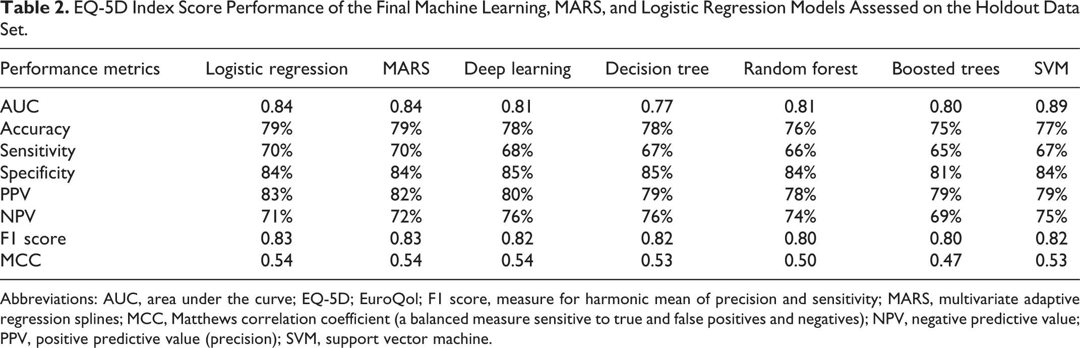
Abbreviations: AUC, area under the curve; EQ-5D; EuroQol; F1 score, measure for harmonic mean of precision and sensitivity; MARS, multivariate adaptive regression splines; MCC, Matthews correlation coefficient (a balanced measure sensitive to true and false positives and negatives); NPV, negative predictive value; PPV, positive predictive value (precision); SVM, support vector machine.
ODI Index Score Performance of the Final Machine Learning, MARS, and Logistic Regression Models Assessed on the Holdout Data Set.
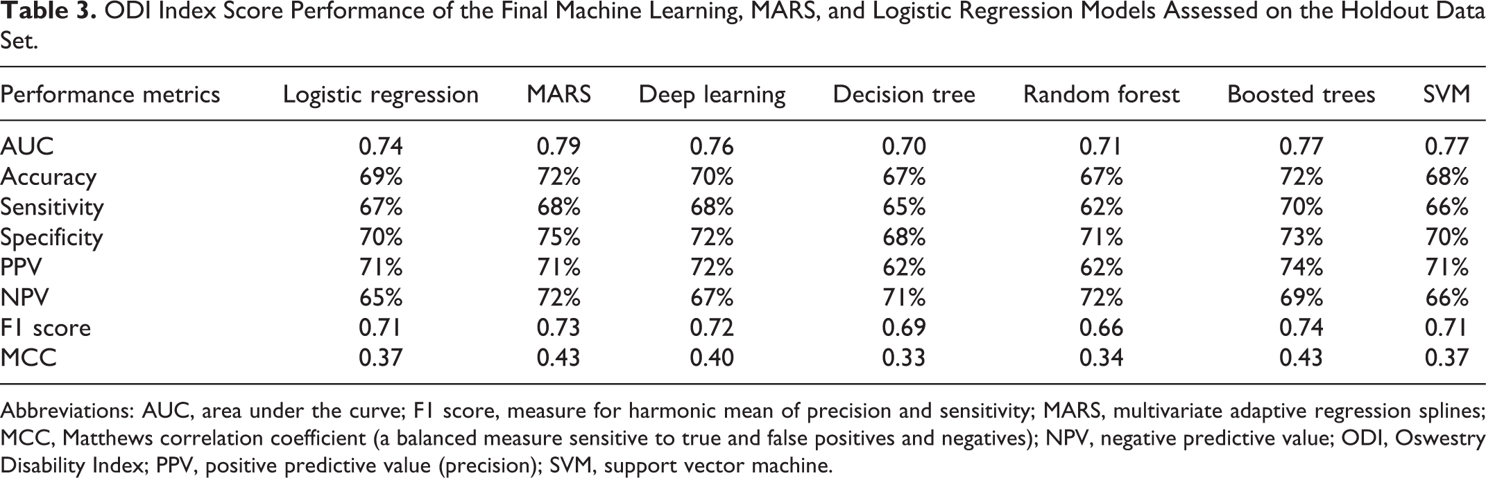
Abbreviations: AUC, area under the curve; F1 score, measure for harmonic mean of precision and sensitivity; MARS, multivariate adaptive regression splines; MCC, Matthews correlation coefficient (a balanced measure sensitive to true and false positives and negatives); NPV, negative predictive value; ODI, Oswestry Disability Index; PPV, positive predictive value (precision); SVM, support vector machine.
VAS Leg Performance of the Final Machine Learning, MARS, and Logistic Regression Models Assessed on the Holdout Data Set.
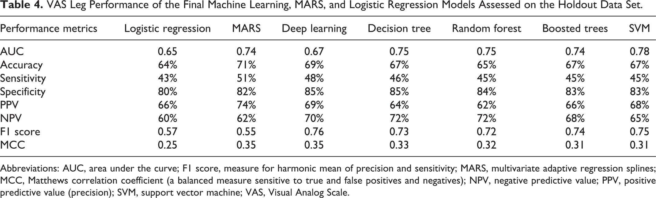
Abbreviations: AUC, area under the curve; F1 score, measure for harmonic mean of precision and sensitivity; MARS, multivariate adaptive regression splines; MCC, Matthews correlation coefficient (a balanced measure sensitive to true and false positives and negatives); NPV, negative predictive value; PPV, positive predictive value (precision); SVM, support vector machine; VAS, Visual Analog Scale.
VAS Back Performance of the Final Machine Learning, MARS, and Logistic Regression Models Assessed on the Holdout Data Set.
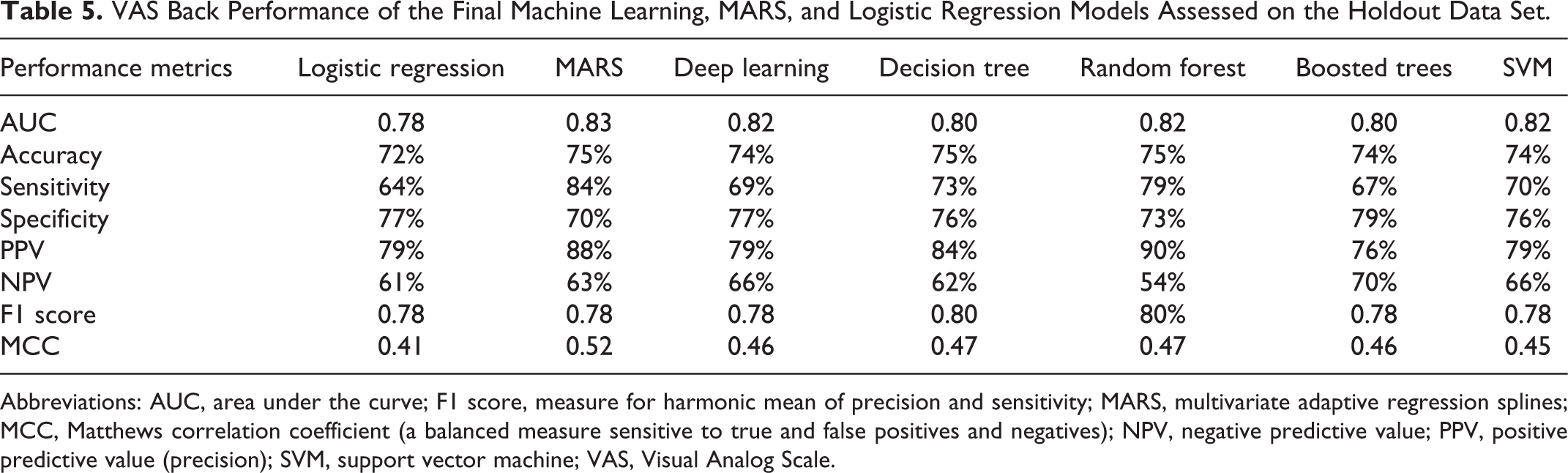
Abbreviations: AUC, area under the curve; F1 score, measure for harmonic mean of precision and sensitivity; MARS, multivariate adaptive regression splines; MCC, Matthews correlation coefficient (a balanced measure sensitive to true and false positives and negatives); NPV, negative predictive value; PPV, positive predictive value (precision); SVM, support vector machine; VAS, Visual Analog Scale.
Return to Work Performance of the Final Machine Learning, MARS, and Logistic Regression Models Assessed on the Holdout Data Set.
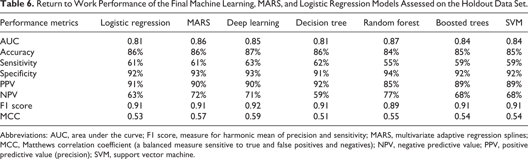
Abbreviations: AUC, area under the curve; F1 score, measure for harmonic mean of precision and sensitivity; MARS, multivariate adaptive regression splines; MCC, Matthews correlation coefficient (a balanced measure sensitive to true and false positives and negatives); NPV, negative predictive value; PPV, positive predictive value (precision); SVM, support vector machine.
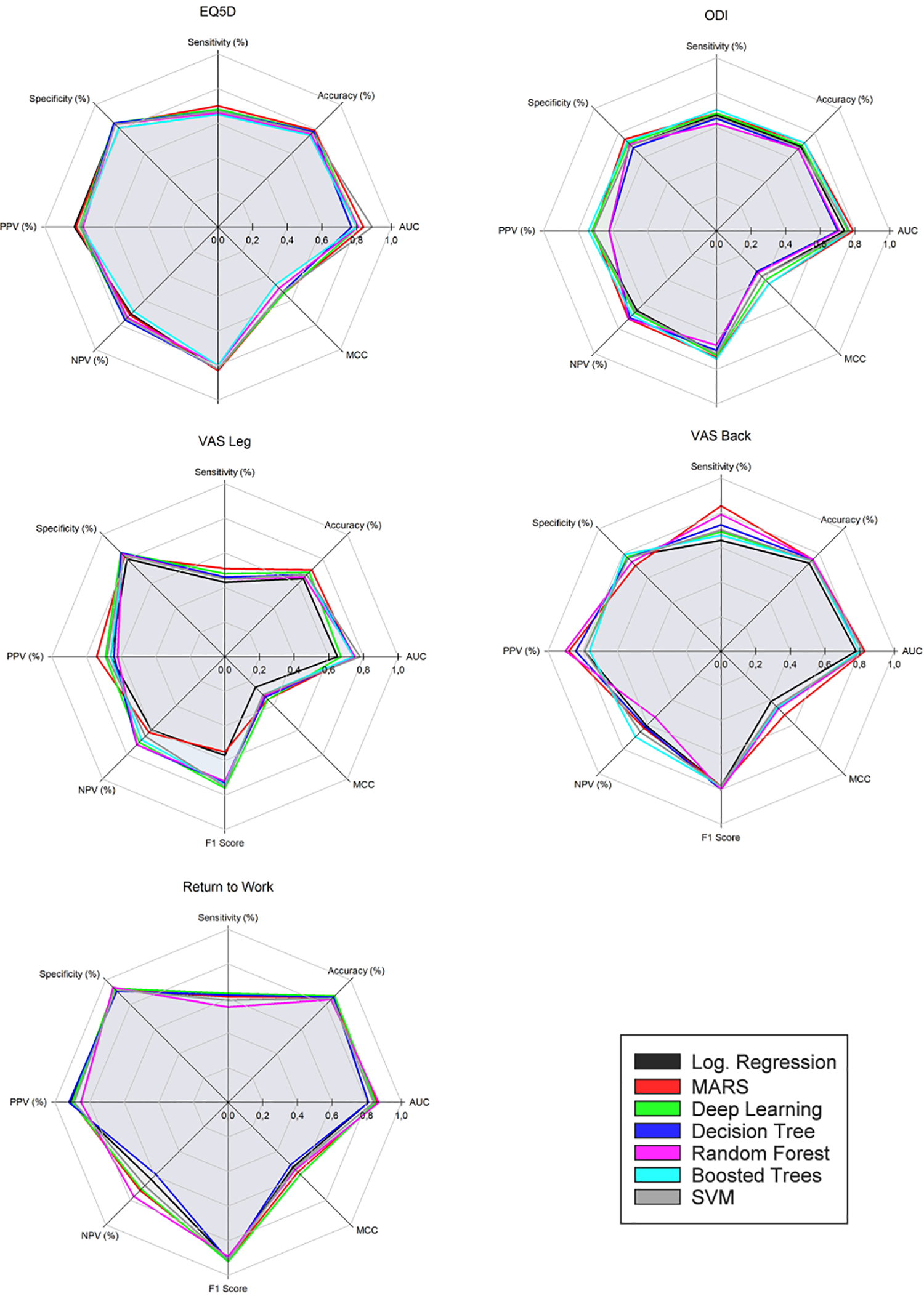
Performance metrics for models: EQ5D, ODI, VAS Leg, VAS Back, Return to Work.
Improvement in EQ-3D at 1 year (positive predictive value [PPV]) was predicted with an average accuracy of 80% (median = 79%; range = 5%). The mean AUC value was 0.82 (median = 0.81; range = 0.12). Nonimprovement (negative predictive value [NPV]) was predicted with an average accuracy of 73% (median = 74%; range = 7%). LR and MARS models performed on par with the best performing ML models.
Improvement in ODI at 1 year (PPV) was predicted by the models with an average accuracy of 69% (median = 71%; range = 12%). The mean AUC value was 0.75 (median = 0.76; range = 0.09). Nonimprovement (NPV) was predicted with an average accuracy of 69% (median = 71%; range = 12%). MARS performed on par with the best performing ML models. LR performed poorly but better than the worst performing ML models.
Improvement in VAS Leg at 1 year (PPV) was predicted by the models with an average accuracy of 67% (median = 66%; range = 12%). The mean AUC value was 0.73 (median = 0.74; range = 0.12). Nonimprovement (NPV) was predicted with an average accuracy of 67% (median = 68%; range = 12%). MARS performed on par with the best ML models. LR did not perform well.
Improvement in VAS Back at 1 year (PPV) was predicted by the models with an average accuracy of 82% (median = 79%; range = 14%). The mean AUC value was 0.81 (median = 0.82; range = 0.05). Nonimprovement (NPV) was predicted with an average accuracy of 63% (median = 63%; range = 16%). MARS performed on par with the best performing ML models. The performance of the LR model was inferior.
Whether patients were successfully able to return to work at 1 year (PPV) was predicted by the models with an average accuracy of 89% (median = 90%; range = 7%). The mean AUC value was 0.84 (median = 0.84; range = 0.06). Nonsuccess (NPV) was predicted with an average accuracy of 68% (median = 68%; range = 18%). MARS performed on par with the best ML model. The LR model performed slightly worse than the least successful ML models.
Discussion
The ML methods applied in this study did not yield overall superior performance compared with the conventional methods. Performance of MARS was on par with the best performing ML method, deep learning. MARS and deep learning models performed consistently well across outcome measures. Mixed results were observed across outcome measures for both LR and other ML models. Discrepancy in performance measures was greatest among the models predicting leg pain improvement. In some cases, ML methods were slightly outperformed by the logistic regression models. One possible explanation for the results may be attributed to the univariate correlations found during model training. This suggests that outcome is linearly related to the severity of patients’ health status preoperatively. That is, patients who are worse off tend to improve the most. This is consistent with the findings of Staartjes et al. 2 Previous studies indicate that ML primarily has performance advantages when data exhibit strong interactions between predictors and nonlinearities. 35 The absence of these qualities might explain the failure of ML methods to prove superior in this study.
Transparency Versus Explainability
Parallel to the empirical success of ML methods in recent years, there is a rising concern about their lack of transparency. 36 Complex models such as deep learning are in essence black boxes once they have been trained. Their inner workings are, although accessible, beyond human comprehension and interpretation. Complex models are often more accurate, but less interpretable and vice versa. 37 Ethically, the problem of explainability is especially important in a clinical setting where patient’s lives and well-being depend on decision-making. 38 It has been well documented that ML can lead to unforeseen bias and discrimination inherited by the algorithms from either human prejudices or artefacts in the training data. 39 Considerable efforts to bridge accuracy and explainability in ML have already been done but remains in its infancy. 40 From an epistemological point of view, the problem of explainability underlines the basic requirement of science to be able to describe the cause and effect of any given system and align the inputs with any given output. Explanatory and predictive accuracy have different qualities and may be viewed as 2 dimensions that all models possess. 41 This suggests that depending on the purpose, trade-offs between transparency and accuracy should be carefully evaluated in model selection. In short, choosing the simpler model might be preferable.
A Priori Model Selection
Several studies have suggested that simple models often perform just as well as more advanced models.42-44 In a recent systematic review including 71 studies (Christodoulou et al 45 ), the authors found no evidence of superior performance of ML over LR. However, they did not investigate which factors might explain this and recommend that future research should focus on identifying which algorithms are optimal for different types of prediction problems. The above-mentioned findings are in line with the theoretical work of Wolpert, 46 which states that averaged across all possible problems, all learning algorithms will perform equally well because of their inherent inductive bias. According to this theorem, there are no objective a priori reasons to favor any algorithm over any others. 46 In conclusion, despite lacking evidence of the superiority of ML, we suggest that clinical prediction should always explore and compare multiple models.
Limitations
The registry used in this single-center study has previously been demonstrated to be unaffected by loss of follow-up. 47 Still, some degree of selection bias cannot be ruled out. No attempt to evaluate missingness of the initial data set (n = 3216) was made, and it was assumed to be missing at random. Consequently, data were not imputed because the final study sample was relatively large. Application of an imputation technique—for example, multiple imputation by chained equations, 48 would have made a larger source of information available to the models, possibly leading to better results. ML techniques appear to require far more data per variable to achieve stability compared with conventional methods such as LR. 49 Comorbidities were not factored in. Neither were surgical methods or complications. Furthermore, to counter overfitting and reduce redundancy, the feature selection was limited to a small subset. Although this strategy could help improve the robustness of the models, it is possible that more predictors could have resulted in a higher degree of accuracy. Finally, the decision in this study to value sensitivity and specificity equally in determining MCIDs is somewhat arbitrary. Prevalence, severity of the condition, and possible adverse effects from treatment should ideally all be considered when deciding an acceptable trade-off between true positives and false positives. 50
Conclusions
We have developed 5 different ML models and 2 conventional models across 5 outcome measures, predicting improvement for patients following surgery for LDH at 1 year after surgery: EQ-5D, ODI, VAS Leg, VAS Back, and Return to Work. The study demonstrates that it is possible to build and train an ensemble of different predictive ML models with little effort and no programming skills, as a starting point for model comparison and further optimization and development. Modern code-free software like RapidMiner may encourage the use of PRO data for predictive purposes by surgeons and other medical professionals by eliminating the need for programming skills.
Footnotes
Declaration of Conflicting Interests
The author(s) declared no potential conflicts of interest with respect to the research, authorship, and/or publication of this article.
Funding
The author(s) received no financial support for the research, authorship, and/or publication of this article.