Sage Journals: Discover world-class research

Abstract

Recent decades have seen increased interest in Cislunar operations. To ensure the safety of flight and peace of operations in the Cislunar domain, a capability to provide current and predictive knowledge of resident space objects in the domain is required, which, in turn, necessitates a dedicated space situational awareness (SSA) system. However, SSA in the Cislunar domain is notoriously difficult to achieve due to the inherently large volume and the chaotic nature of orbits in the regime. These characteristics produce challenges in establishing persistent monitoring and limit predictive capabilities. To address these challenges, this study detailed a trade space for achieving effective Cislunar SSA (CSSA) by leveraging improved capabilities offered through very large (5–10× the size of currently available space-based apertures) radio frequency and optical sensors. The approach presupposes a paradigm shift in space operations that enables on-orbit manufacturing of large, precise structures. We show that access to very large apertures enables timely, persistent, and accurate CSSA through higher signal-to-noise ratios, resolutions, and detection ranges in the operational environment that could not otherwise be achieved by leveraging a proliferated network of many smaller, conventionally sized sensors.

Keywords

Cislunar space situational awareness (SSA)in-space assembly and manufacturing (ISAM)remote sensing

INTRODUCTION

Space situational awareness (SSA) is the ability to provide characterization and predictive knowledge of the space environment through detection and tracking. It encompasses the understanding of the space environment and the ability to monitor activities in space to ensure the safety of operations.¹ A Cislunar SSA (CSSA) capability is currently absent but critically important to ensure the safety of increasing space traffic in that region. Key distinctions between Earth-centric SSA and CSSA include significantly larger observational volumes, weaker illumination leading to lower signal returns, a more complex dynamical environment characterized by non-Keplerian orbits, and greater distances to targets, which demand higher signal-to-noise ratios (SNRs) or enhanced resolution. As a result, traditional Earth-centric SSA capabilities—reliant on ground-based infrastructure and Earth-launched space assets—do not scale efficiently to meet CSSA needs. This challenge opens the door to innovative approaches, such as leveraging in-space assembly and manufacturing (ISAM) as a near-term enabling technology. ISAM could support the fabrication of large-scale sensors (e.g., 100–1,000 meter-class apertures) directly in space, offering a potentially faster and more cost-effective path to operational CSSA capabilities.

In 2022, the White House Office of Science & Technology Policy released a report that outlined the nation’s goals for the development of the Cislunar domain.² Complementary to this, others have investigated specific families of Cislunar orbits to maximize the coverage of targets and volumes in the Cislunar domain. Ongoing research in CSSA viability is exploring the feasibility of both ground and space-based sensors for effectively surveying the Cislunar volume.^3–5 Popular space-based CSSA sensors include radio frequency (RF)⁶ and electro-optical (EO)^7,8 sensors for providing a search/detect/track capability. Conventional RF and EO sensors must function over long operational ranges, which significantly limit their performance. Specifically, RF sensors are plagued by high power consumption to detect distant objects, and EO sensors require proper solar illumination conditions and only cover a volume of space that is commensurate with their field of view (FOV) and have poor resolution.^9–11 These limitations posed by conventional RF and EO sensors make it difficult to establish a CSSA capability.

Advancements occurring within ISAM may offer a solution whereby unconventionally large sensors could be fabricated and assembled on orbit at a fraction of the cost and time that SSA sensors are deployed today. Additionally, an ISAM approach to sensor development removes constraints on sensor size posed by the tyranny of launch (i.e., where components must fit into a rocket fairing and survive a violent launch event) and provides an ideal microgravity environment to allow for the design and manufacturing of exceptionally large structures that require relatively low mass to maintain a high degree of precision. A paradigm shift toward in situ manufacturing of large apertures removes traditional launch constraints and redefines sensor design. Defense Advanced Research Projects Agency (DARPA)’s Novel Orbital and Moon Manufacturing Materials and Mass Efficient Design (NOM4D) program aims to enable space-based systems too large to launch from Earth by developing advanced fabrication techniques. These efforts target high-precision structures, including a 100-m RF reflector. NOM4D could enable 5–10× larger structures than currently possible, unlocking unprecedented SSA capabilities—particularly in the Cislunar domain—through enhanced measurement quality and tracking accuracy.

In light of recent national strategies and commercial plans for Cislunar activity, the need for a scalable and persistent SSA capability is critical. The vastness of the Cislunar domain, which encompasses volumes on the order of 10³ larger than GEO, renders traditional Earth-based SSA systems insufficient. Thus, this study explores advanced concepts that may be realized through maturing ISAM technologies motivated by NOM4D. This article discusses a process for modeling and simulating the Cislunar domain to evaluate the performance of very large sensors for CSSA. CSSA in this context was decomposed to the ability to search/detect/track/recognize objects, resulting in the ability to maintain custody, distinguish objects from others, and recognize objects as belonging to certain types. The development of a CSSA architecture required an understanding of both the dynamics of the Cislunar environment (orbital modeling and architecture development) and the physics of the sensors (sensor modeling). Therefore, we detail a trade space considering sensor design (active/passive RF and passive optical), aperture size, sensor number, and sensor location.

MATERIAL AND METHODS

Key CSSA Capabilities: Search, Detect, Recognize, Track

The performance of each sensor type was evaluated in order to inform how well it executed a specific SSA capability including search, detection, recognition, and tracking (Table 1). In the context of this investigation, the search capability involved systematically scanning a defined volume of space to locate objects of interest. Effective searching depended on the sensor’s coverage area and its ability to scan the full 4π sr (referring to the angular FOV for observing the entire surface of a sphere from its center measured in steradians [sr]) space. Sensors performing a search capability were not queued by other sensors on where to look for resident space objects (RSOs). Detection referred to the sensor’s ability to make out the presence of an object within its FOV. This involved distinguishing potential objects from background noise and is quantified by metrics such as SNR, probability of detection (p_d), and false alarm rate (p_fa). Sensors performing detection were assumed to be queued (refered to as perfect pointing) from other sensors and therefore knew where to look to detect an RSO. Recognition assumed perfect pointing and was characterized as the ability to not only detect an object but also classify it, determining its type or category, such as a satellite, debris, or other space objects. For this investigation, recognition was limited as an optical capability that was reliant on the sensor’s resolution and was therefore related to the image quality (rather than purely the SNR). The Johnson Criteria¹² were used to define the ability of an imaging sensor to perform recognition.^13,14 The Johnson Criteria were selected over alternatives such as the National Imagery Interpretability Rating Scale (NIIRS) because it provided a physics-based, resolution-driven metric that could be directly applied to modeling optical detection and recognition performance in the Cislunar regime. NIIRS, on the contrary, is a task-based scale tied to Earth-observing imagery interpretation and was less transferable to this context. Finally, tracking (also assumed perfect pointing) involved continuously monitoring the detected objects over time to determine their trajectory and predict future positions. This required high-accuracy measurements to maintain accurate and consistent tracks. All together, these performance aspects determined the overall effectiveness of sensors in maintaining SSA, enabling timely and informed decision-making for space operations and safety.

Table 1.

Four sensor types were investigated to provide a specific CSSA capability. The table maps each phenomenology to its optimal CSSA capability (search, detection, recognition, tracking)

Sensing Modality	Search	Detection	Recognition	Tracking
Small optical (passive)	X	X
Large RF (active)	X			X
Large RF (passive)		X
Large optical (passive)			X

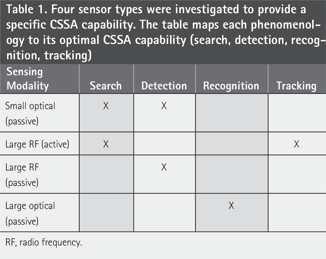
RF, radio frequency.

Sensor Models

To explore the ability of large optical and RF sensors to support CSSA, sensor models were developed that provided first-order information on the operational range, spatial and range resolution, and FOV. The RSO in the analysis was defined as an aluminum cylinder with a height of 10 m and a radius of 1.25 m. This was representative of a large Cislunar spacecraft equipped with solar panels, similar to the National Aeronautics and Space Administration’s DART spacecraft, which had large solar panel arrays that were 8.5 m long when fully deployed.¹⁵ Figure 1 shows a representation of how an optical sensor may image the RSO at a wavelength of 800 nm at different operational ranges, adapted from our previous work.³ For the active RF sensors, the RSO defined corresponded to a radar cross section (RCS) of 7,854 m². The transmission parameters of the RSO are defined further within the passive RF sensor model (Section “Large Passive RF (p-RF) Sensors (Detection)”).

Fig. 1.

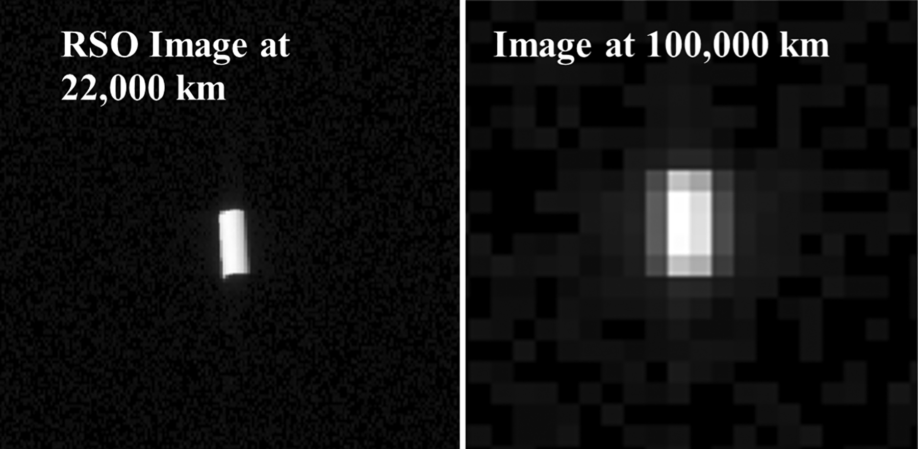
Synthetic optical images generated for a 10 m tall cylindrical RSO imaged by an 800 nm optical sensor with a 100 m aperture at a range of 22,000 km and a range of 100,000 km adapted from DeCoster et al.³ RSO, resident space object.

Small passive optical sensors (search + detect)

The performance of CSSA architectures comprised of conventionally sized (small) optical apertures operating at 800 nm was investigated for providing a search capability within the Cislunar domain to justify the perfect pointing (sensors were queued on where to look) operation of the large passive RF and optical sensors. An overview of the sensor models is provided here, with further detail provided in the Supplementary Data.

The performance of small optical sensors to provide a search and detection capability was based on the SNR (i.e., how many photons from the RSO made it to the detector) rather than their ability to form a high-quality image. For this analysis, SNR (rather than resolution) was used as the metric to define whether the sensor could achieve search and detection of an RSO. For this analysis, illumination was fixed to a favorable Sun–object–sensor geometry (α ≈ 0°) to provide an upper-bound detection range. Note, however, that in general, SNR scales with the solar phase angle through the target phase function Φ(α) used in the optical model. The architecture-level analysis and results incorporated illumination and exclusion effects within the SSA simulation framework. Table 2 details the sensor model parameters used to describe the small passive optical sensors.

Table 2.

Optical sensor model parameters used in the search and detection analysis. The focal plane array (FPA) size was set to 10,000 x 10,000 pixels. Parameters relevant to the SNR calculation, including pixel pitch, aperture diameter, quantum efficiency, and FPA size, are included for completeness and repeatability

Optical Sensor Model Parameters
Wavelength	800 nm (VIS)
Waveband	400–1,000 nm
Reflectivity	98%
Solar phase angle (α)	0^o (fully lit)
Aperture diameter (m)	10 cm and 1 m (search cases)
Pixel pitch	4.6 μm
Quantum efficiency	60%
Detector integration time	1 ms
Detector response time	11 ms (Si detector)
Atmospheric transmittance (%)	100 (space-based)

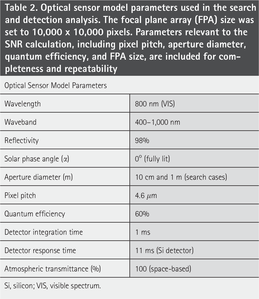
Si, silicon; VIS, visible spectrum.

Large active RF sensor platform (search/detection and tracking)

The performance of an active RF sensor platform comprised of eight individual active RF sensors designed for performing search/detection and tracking within the Cislunar domain was investigated. An RF sensor platform comprised of eight apertures exhibited a search capability whereby each of the eight RF sensors scans one-eighth of the search volume and thereby decreases the scan time to search the full volume. The active RF sensor platform is illustrated in Figure 2. It was comprised of eight RF apertures that each had a diameter of 100 m. Each RF sensor was placed at the corner of a 125 m cube on a mechanical mount that allowed for one-eighth of the full 4π sr pointing for each aperture. One face of the cube was assumed to point at the Sun and carried a large solar array to provide the necessary power to the RF platform (up to 3 MW).

Fig. 2.

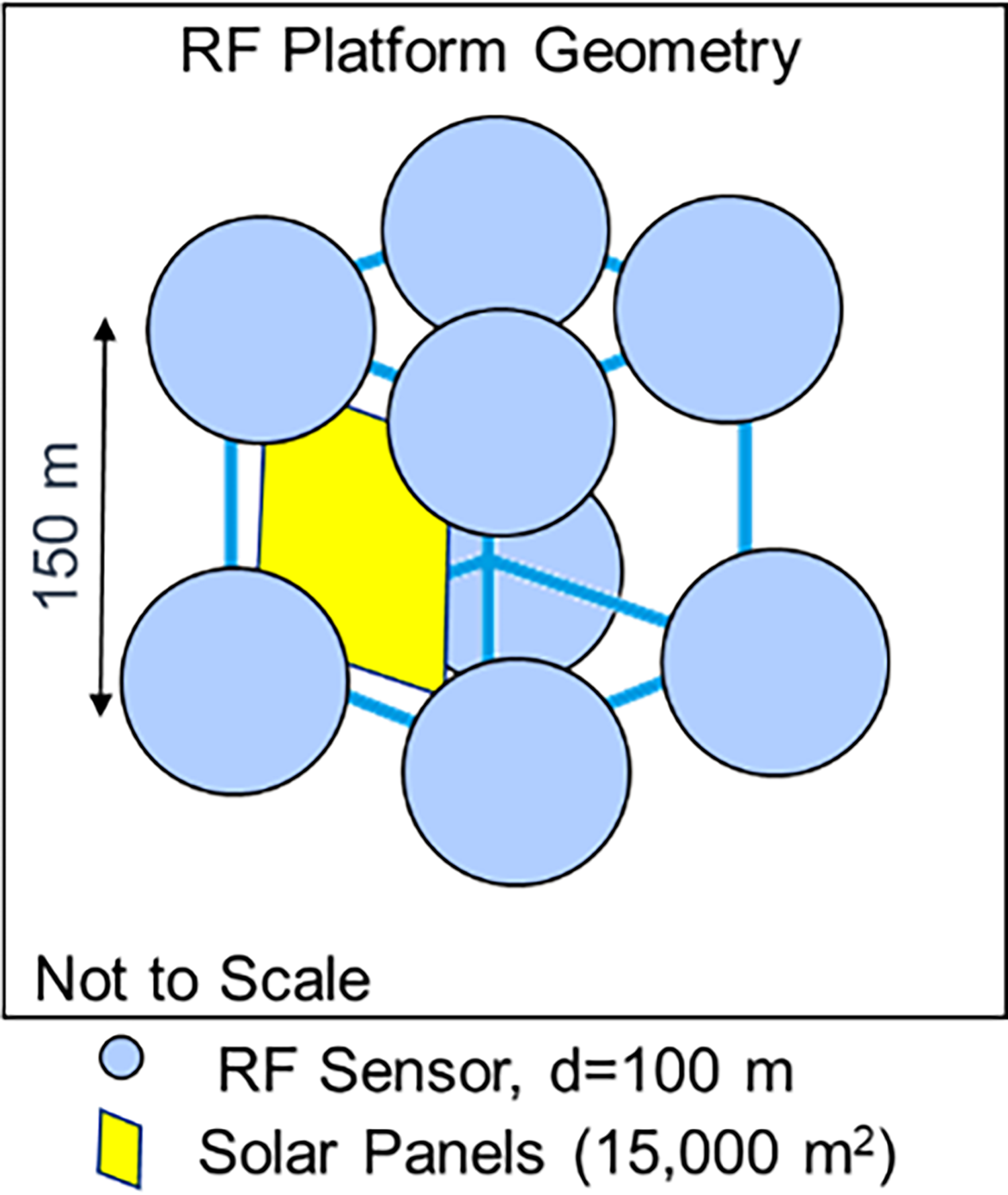
Illustration of the active radio frequency (RF) platform comprised of eight RF sensors (each had a diameter of 100 m), mounted on the vertex of a cube. One face of the cube contained solar panels that were always facing the Sun and provided sufficient power to the platform.

Table 3 shows the parameters used to describe the active RF sensor model. The RF system operated in a radar configuration capable of coherent integration of pulses. The radar performance was quantified in terms of the system’s ability to detect a target of 7854 m² (corresponding to a 10 m tall cylindrical RSO) RCS with a probability of detection (P_d) of 95% and a probability of false alarm (P_fa) of 10⁻⁴, for each look direction. These performance metrics were based on previous studies that cover radar detection performance metrics.^16,17 Coherent detection theory demonstrated that an SNR of 11.6 dB was required to achieve the desired detection performance.¹⁶ The radar range equation was used to obtain the scan time required to cover 4πsr of search volume as a function of the two-way time of flight of a single RF pulse, aperture diameter for a given SNR, average radiated power, noise power, RSO RCS, integration time, and radar range to target.¹⁴ See Supplementary Data, for further details.

Table 3.

Active RF sensor model corresponding to a single RF sensor. The active RF sensor was capable of integrating 100 pulses (taken to be chirps) over a CPI of T, that had a minimum value of T_min where the minimum scan time performance was achieved as a function of aperture diameter (D)

Active RF Platform Sensor Model Parameters
Frequency	3 GHz (S-Band)
Wavelength (λ)	0.1 m
SNR	11.6 dB
Probability of detection	95%
Probability of false alarm	10⁻⁴
Aperture efficiency	0.7
Average transmit power per sensor	37.5 kW
Radar cross section (RCS) (σ) of cylindrical RSO	7,854 m²
Noise temperature (T_o)	185 K
Chirp constant (α)	1 × 10¹⁰ Hz/s
Beamwidth	(λ/D)
Bandwidth (B)	10 MHz
Pulse length (τ)	1 ms
Duty cycle (pulse width/PRI)	1
T_l (two-way travel time at 100,000 km)	667 ms
T_min minimum CPI (T) time	100 ms

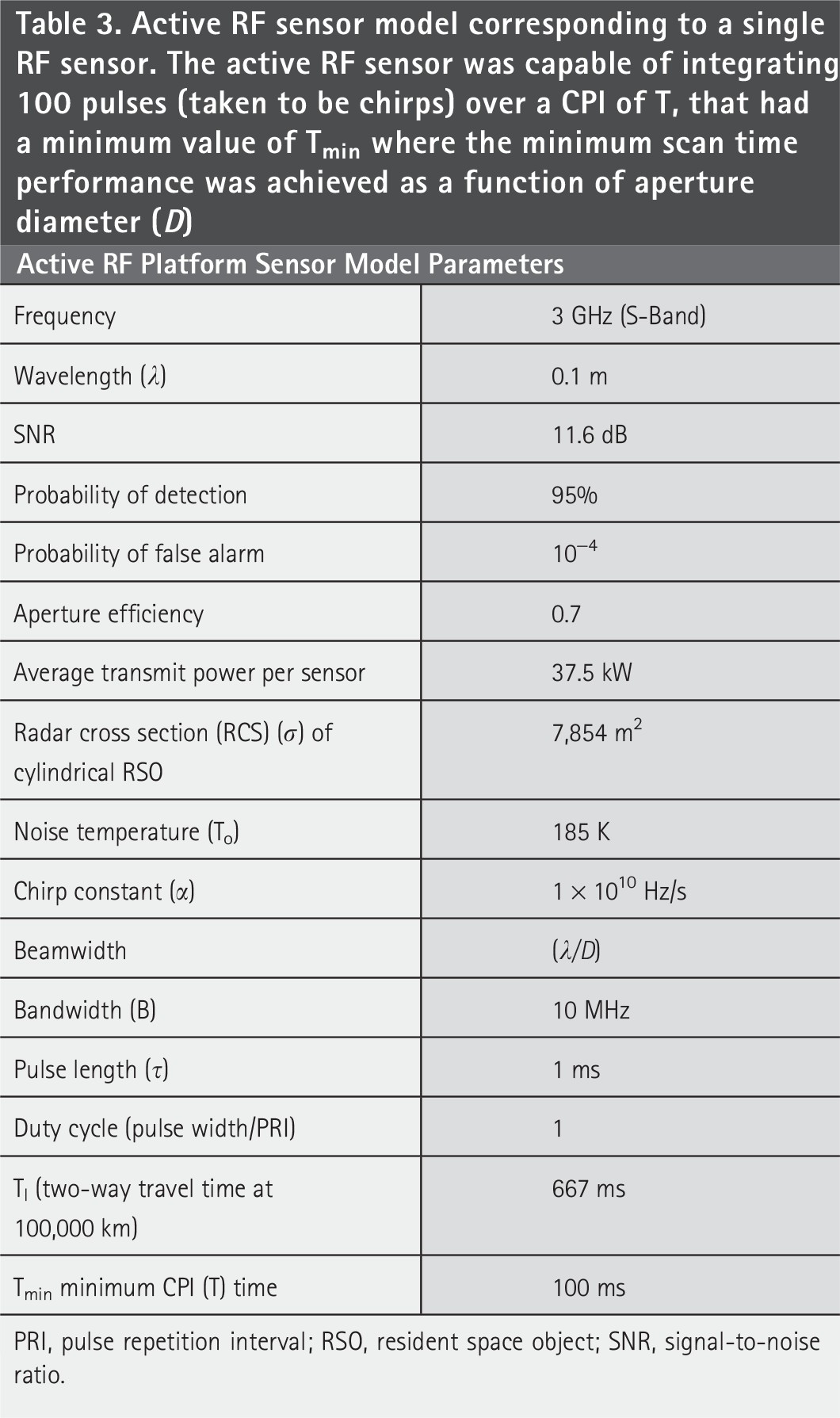
PRI, pulse repetition interval; RSO, resident space object; SNR, signal-to-noise ratio.

Large passive RF (p-RF) sensors (detection)

Large passive RF sensors were identified as an ideal sensor to provide a CSSA detection capability since they were not limited by power, and the SNR at the receiver was improved by a larger sensor size. Therefore, a passive RF sensor model was developed in order to investigate the role of large passive RF sensors for providing a Cislunar detection capability. Detection for passive RF sensors was performed based on the RF signal radiated by the RSO to be detected. When the RSO was intentionally radiating RF signals, the passive signal intercepted by the passive detector was typically received through the side lobes (secondary radiation patterns that appear around the main lobe that were less intense), rather than the main beam, of the platform antenna. Figure 3 shows an example of a realistic RF parabolic receiver pattern and the simplified ellipsoid pattern modeled for this investigation, where the main lobes point to 0°.

Fig. 3.

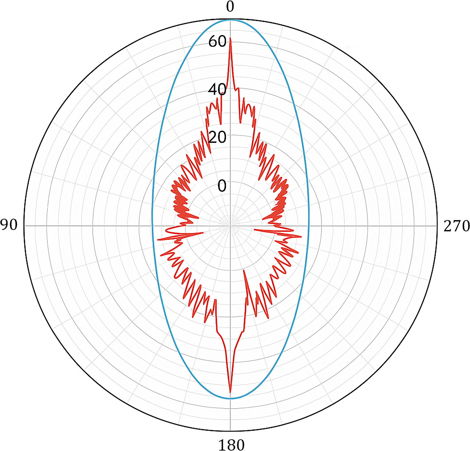
Polar diagram of a nominal RF parabolic receiver pattern (red).¹³ The blue pattern shows the simplified ellipse pattern that was input into the SSA simulation. The main lobe extended to 5 W, and the side lobes extended to 0.05 W for the simulated transmitter. SSA, space situational awareness.

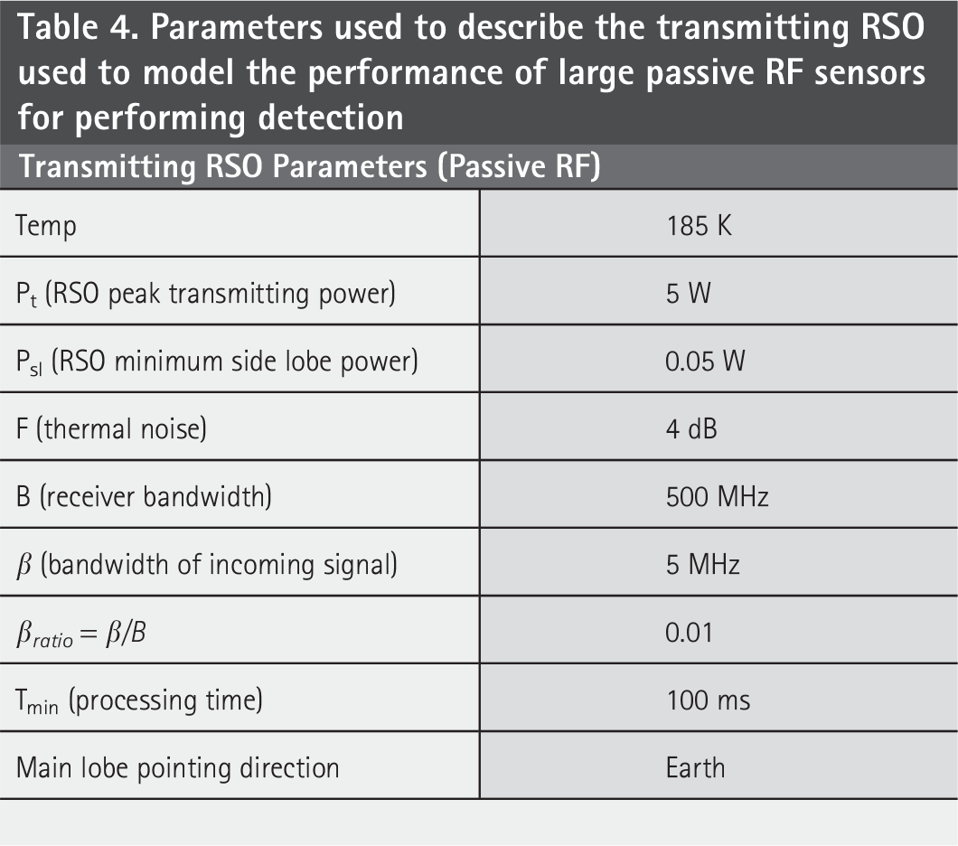
An important distinction between passive and active RF detection was that in passive detection, the detector has no a priori knowledge of the form of the signal to be intercepted. Therefore, the coherent combination of pulses to improve the SNR via matched filtering required additional processing to estimate the phase of the incoming signal.¹⁸ It was assumed that this type of processing was available, and therefore, the passive RF sensors were capable of performing coherent detection. Table 4 details the parameters used to describe the emitting RSO used to model the detection performance of the architecture of passive RF sensors. Note that to be effective, the bandwidth of the incoming signal (β) had to be smaller than the receiver bandwidth (B). The maximum RSO transmit power was set to 5 W (in the main beam). This was in the range of typical deep space transponders that could be used on Cislunar RSOs, such as JPL’s Iris 2.0 X-band transponders capable of 4 W RF output power.¹⁹ Additionally, previous Cislunar missions such as Lunar Flashlight (6U CubeSat) and the Near-Earth Asteroid Rendezvous used telecom hardware ranging from 1 to 9 W of peak power.^20,21 See Supplementary Data, for further details on the passive RF sensor development and modeling.

Table 4.

Parameters used to describe the transmitting RSO used to model the performance of large passive RF sensors for performing detection

Transmitting RSO Parameters (Passive RF)
Temp	185 K
P_t (RSO peak transmitting power)	5 W
P_sl (RSO minimum side lobe power)	0.05 W
F (thermal noise)	4 dB
B (receiver bandwidth)	500 MHz
β (bandwidth of incoming signal)	5 MHz
β_ratio = β/B	0.01
T_min (processing time)	100 ms
Main lobe pointing direction	Earth

Large passive optical sensor model (recognition)

The use of large passive optical sensors for providing a recognition CSSA capability was investigated because large apertures provide high resolutions over long ranges. The performance of the optical sensors described here was predicated on the Johnson Criteria.¹⁴ Johnson uses an imager’s resolving power as the metric for target acquisition. For a given target-to-scene contrast, the resolving power (highest spatial frequency) was multiplied by the object size to define the minimum number of pixels across the object to perform recognition. The Johnson Criteria characterize the probability of an ensemble of observers having a 50% chance of discriminating an object based on the effective resolution of an imaged object. This study employed the Johnson Criteria using apertures ranging in size from 10 m to 1,000 m in diameter. The Johnson Criteria for 50% probability utilized for this analysis assumed that recognition required 13 × 5 pixels, which corresponded to a minimum resolution of 0.77 m/pixel (10 m object/13 pixels).

The details of the optical sensor model developed for this study are shown in Table 5. An optical wavelength (λ) of 800 nm was chosen to assess the performance of optical sensors operating in the visible spectrum (VIS). Note that if the RSO was warm (≥300 K), then from an SNR perspective, long-wave infrared (LWIR) (∼8–14 μm) sensors would be superior to VIS sensors because self-emission from the warm RSO would provide more photons to the detector than photons reflected off the RSO from the Sun. However, since this investigation assessed the ability of large optical apertures to perform recognition (i.e., image quality), VIS was superior to LWIR because the image resolution scaled as λD⁻¹, where D was the diameter of the optic (Fig. 11). Therefore, an optical sensor operating at 800 nm (VIS) would have roughly 10× better resolution than an optical sensor operating at 10 μm (LWIR) at the same range (assuming favorable viewing geometries with respect to the Sun). However, due to the anticipated mirror roughness (∼1 μm) defined by the NOM4D program metrics, the calculated resolution was artificially degraded by a factor of 3.

Table 5.

Parameters for the large passive optical sensor model designed for recognition. The focal plane array (FPA) size was 10,000 x 10,000 pixels

Optical Sensor Model Parameters
Wavelength	800 nm (VIS)	10 μm (LWIR)
Diameter (m)	10, 100, 200, 300, 400, 500, 1,000
Atmospheric/space transmittance	100%
Quantum efficiency	60%
Detector integration time (ms)	1	1
Detector response time (ms)	11 (Si)	1 (HgCdTe)
Pixel size (μm)	4.6	12
FPA size (pixels)	10,000 × 10,000
Blur factor	3	1
Reflectivity (%)	98	98

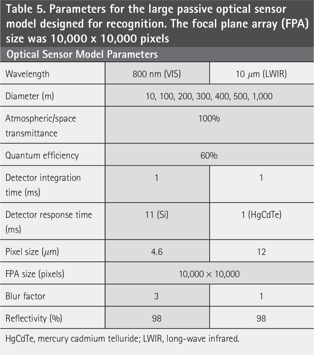
HgCdTe, mercury cadmium telluride; LWIR, long-wave infrared.

Cislunar Observer Orbits

Cislunar space is defined as the volume of space where objects are under the gravitational influence of both the Earth and the Moon. Holzinger, Chow, and Garretson 2021 illustrate the scale of the Cislunar volume, which extends far beyond geosynchronous orbit (GEO), within their Figure 2.²² Not only is the Cislunar region vast (spanning 100,000 km), but orbits in this domain are difficult to predict and model. The Cislunar region is characterized by chaotic dynamics due to gravitational effects from the Earth, the Moon, and the spacecraft (three-bodies), so orbits cannot be accurately described using classical Keplerian orbital elements.^23–25 Although the Cislunar domain is inherently chaotic, requiring numerical propagation and solvers to predict orbital dynamics, there are special cases that result in stationary or nearly periodic orbits. For example, the Earth–Moon system in the framework of the Circularly Restricted Three-Body Problem (CR3BP) contains five stationary points, known as the Earth–Moon Lagrange points.²⁶ Additionally, certain trajectories near the Moon and Lagrange points, called repeating natural or periodic orbits, nearly retrace their path over a fixed time interval. Although orbits in the Cislunar regime are dynamically complex, this investigation took advantage of simplified sensor architectures comprised of semi-stable orbits such as DROs and Lagrange point halos. These orbits required station keeping, but at relatively low ΔV budgets. We cite recent analyses indicating that such orbits were feasible for long-duration operations with modest propulsive corrections.^27–29 While these orbits offer semi-stability that incur lower station keeping costs, sensors placed in these orbits still must overcome long operational distances, nonconstant solar illumination, and large search volumes.

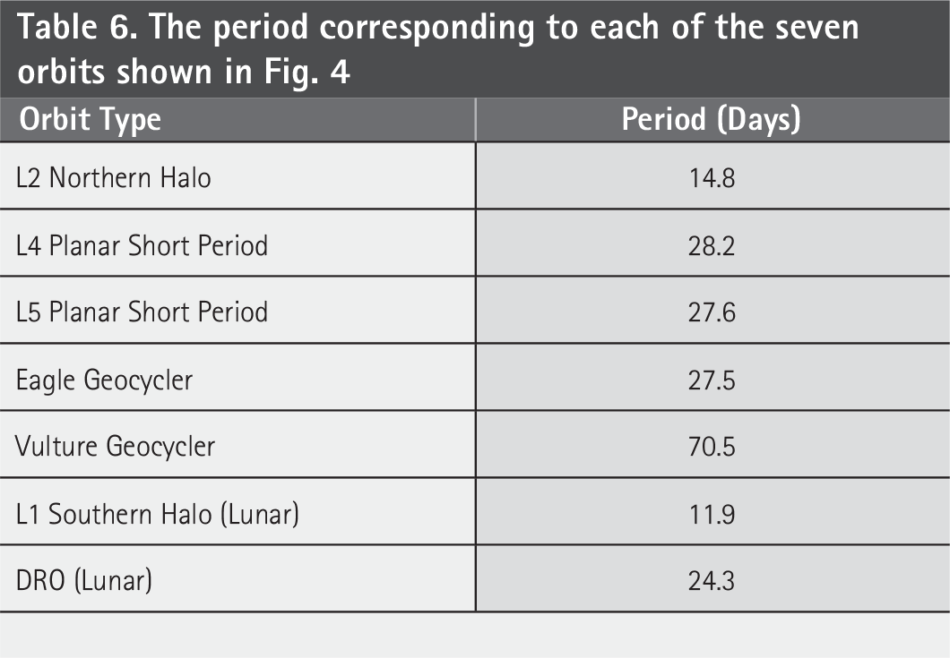
The CR3BP formulation was used to describe the dynamics of Cislunar orbits defined in this investigation. The spacecraft’s mass was assumed to be negligible compared to the Earth and Moon, which were treated as point masses. Additionally, the Earth and Moon were assumed to have circular orbits around their barycenter with constant distance, and the dynamics were described in a rotating synodic frame, making them time-invariant.³⁰ Table 6 and Figure 4 detail and illustrate the periodic orbits selected to construct the eight CSSA architectures defined in this study. These specific orbits were chosen to provide spatial and geometric diversity across the domain.

Fig. 4.

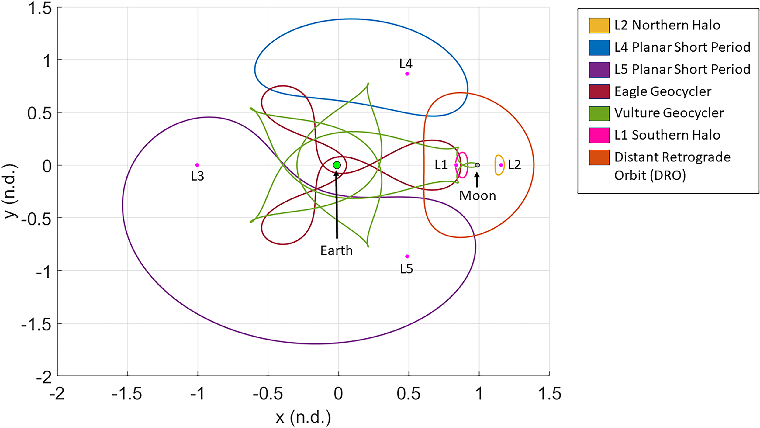
Illustration of the seven orbits within the CR3BP used to construct the eight Cislunar SSA architectures detailed in Table 7. The spatial scale was 1:384,000 km. CR3BP, Circularly Restricted Three-Body Problem.

Table 6.

The period corresponding to each of the seven orbits shown in Fig. 4

Orbit Type	Period (Days)
L2 Northern Halo	14.8
L4 Planar Short Period	28.2
L5 Planar Short Period	27.6
Eagle Geocycler	27.5
Vulture Geocycler	70.5
L1 Southern Halo (Lunar)	11.9
DRO (Lunar)	24.3

Table 7.

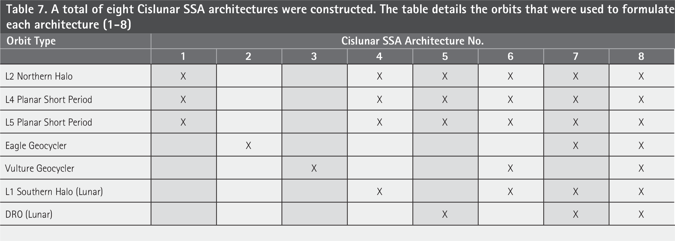
A total of eight Cislunar SSA architectures were constructed. The table details the orbits that were used to formulate each architecture (1-8)

Orbit Type	Cislunar SSA Architecture No.
	1	2	3	4	5	6	7	8
L2 Northern Halo	X			X	X	X	X	X
L4 Planar Short Period	X			X	X	X	X	X
L5 Planar Short Period	X			X	X	X	X	X
Eagle Geocycler		X					X	X
Vulture Geocycler			X			X		X
L1 Southern Halo (Lunar)				X		X	X	X
DRO (Lunar)					X		X	X

CSSA Performance

Modeling area coverage performance

The CSSA architecture performance analysis leveraged a tool developed by the Johns Hopkins University Applied Physics Laboratory called the Comprehensive Analysis Tool Kit (CATK). CATK is a medium-fidelity physical modeling and end-to-end SSA analysis capability. CATK is capable of generating, modeling, and analyzing multi-modal and multi-static SSA architectures, which can include ground stations on the Earth and the Moon, as well as orbiting observers around the Earth, the Moon, or in Cislunar space. The analysis presented in this article was underpinned by CATK’s ability to accurately model naturally occurring exclusion zones within the Cislunar domain (i.e., eclipse, solar exclusion) as well as EO, infrared, and radar (RF) systems detection capabilities. For the passive RF analysis, the detection performance was based on the SNR measured by the passive NOM4D-enabled RF receiver. For the optical analysis, the ability to recognize an object was based on the image quality produced by the NOM4D sensor, which was detailed previously. Each architecture configuration was evaluated with CATK on a 2D Cislunar grid over 30 days with 1-day time steps. At each grid/time sample, the line-of-sight was computed in addition to naturally occurring exclusion zones (eclipse, solar exclusion, Earth/Moon occlusion/occultation), followed by the evaluation of sensor-specific physics: SNR-based detection (RF and small optical models) and Johnson Criterion recognition (resolution threshold; ≈13 × 5 pixels ≡ 0.77 m/pixel). The percent area coverage (time- and/or spatially averaged) was reported as the scalar performance metric per configuration.

In the analysis presented here, an evenly spaced 2D grid was generated across the area of interest in Cislunar space. A representative RSO was assumed to be positioned at every spatial grid point so that the final result quantified what percentage of the area (2D) an SSA architecture could detect or recognize an object. By defining an architecture, a sensor model that was dependent on the RSO characteristics, and a simulation time, CATK computed all the exclusion zones (solar exclusion, Earth/Moon shadow, Earth/Moon occlusion, Earth/Moon occultation) and signal (i.e., SNR or image quality) at each time step and evaluated how well the space was observed by the entire architecture. In order to compute both exclusion zones, as well as radiometric quantities, the location of the observer and key astronomical bodies, such as the Sun, had to be known. CATK leveraged JPL NAIF’s SPICE toolkit^31,32 to bookkeep and produce these values.

CATK produced multiple metrics based on the CSSA analysis, such as time-averaged coverage, spatially averaged coverage, total architecture detection performance, time between detections, and time until first detection for each point in the grid. These metrics were inherently valuable to understanding the performance of the architecture and were leveraged as objective functions to further optimize important parameters, such as observer orbit, orbit phasing, and sensor selection. These parameters were used to compare and contrast various SSA architectures (that could be NOM4D-enabled).

Table 7 details the eight CSSA architectures constructed from the orbits illustrated in Figure 4. For each architecture, we placed either optical or passive RF sensors into each orbit and varied both the sensor size (diameter ranged from D = 1, 10, 100, & 1,000 m) and sensor number (N = 1–50) per orbit. In the case where we placed one sensor per orbit (N = 1), the starting position of each sensor was randomly chosen. Subsequent sensors (N >1) were then placed into each orbit so that they were spaced equidistant from one another. Furthermore, the 2D simulation grids of the CATK models were spatially (Δx = 4,000 km) and temporally (Δt = 1 day) discretized, and the total simulation time for each architecture was 30 days (roughly equivalent to a lunar month). For the context of this study, the Cislunar area was defined by a 1,152,000 km × 1,152,000 km square centered on the Earth, for a total area of 1.33 × 10¹² km².

Machine learning analysis

In this work, we use a random forest regressor³³ to predict the simulated area coverage from inputs of interest (sensor number, sensor diameter, architecture ID). Data were split 80/20 (train/test), and the model fidelity was assessed by comparing predicted versus true targets. Permutation importance (10 repeats) was used to evaluate variable influence. The random forest model served as a surrogate for interpretability and interpolation of the physics-based results. It was not used for classification or optimization. We employed the random forest implementation in the scikit-learn³⁴ Python package and used the default hyperparameters and settings (e.g., 100 estimators and squared error minimization).

In order to train the random forest model, a given dataset (e.g., passive RF detection rates) was randomly split into training and testing folds, using 80% of the data for training and the remainder for testing. We treated sensor number and sensor diameter as continuous variables while using a one-hot encoding to expand architecture type into a set of binary variables. The performance of the random forest model was assessed by comparing the predicted versus true target for each dataset. The model demonstrated a high degree of accuracy, attaining an R² ≥0.993 across all prediction metrics.

The random forest surrogate was used to assess variable importance. The mechanism we used to assess the impact of input variables (such as sensor size or sensor number) on output variables (such as detection rate) was permutation importance³³ via the implementation in scikit-learn. Permutation importance is a common way of assessing variable importance for random forest models. This analysis was based purely on correlations that exist in the data and cannot uncover or take into account the causal mechanisms that generate the data. In future work, we could use causality-aware methods like Bayesian networks³⁵ to further understand the causal influences (like the effects of illumination) on the data.

With the permutation importance method, we took each dataset’s testing fold and iterated through its input variables. We randomly permuted the input variable’s values and then calculated the change in accuracy (in terms of the mean absolute error across the test set) for predicting the output with the permuted variables. This change, measured in units of a given output variable, was thus interpreted as a measure of how important a given variable was for predicting the output, and the results could be compared across all input variables. Because the method was random (based on the permutation), the assessed importance was also random. For each dataset, we repeated the permutation analysis ten times and reported the average permutation importance (see Section “Results,” Fig. 15).

RESULTS

Enabling Perfect Pointing with Small Optical and Large Active RF Sensors

The performance of CSSA architectures composed of small conventionally sized optical sensors and platforms of large active RF sensors was investigated for providing a search and track capability to queue large passive RF and optical sensors to provide a detection and recognition capability. The results below showed that certain phenomenologies were well suited for providing a search, detection, recognition, or tracking capability. In brief, a proliferated network of smaller optical sensors provided an unmatched search capability due to their large FOVs and short scan times required to search large volumes of space. Large active RF sensors provided high-accuracy tracking measurements that allowed for custody to be maintained 100% of the time. Next, large passive RF sensors were well suited for performing detection because their large receiver permitted a high SNR of very low transmit powers across long operational ranges. Additionally, large optical sensors offered the advantage of high resolution over long operational ranges, which provided sufficient image quality to recognize objects within the Cislunar domain.

Small optical sensors (search)

The relationship between FOV, scan time, and sensor diameter for optical sensors is shown in Figure 5. Smaller optical sensors were well suited for searching a large volume because they had a large FOV and therefore much faster scan times for providing a search capability. Figure 5 indicates that a 10 cm diameter optical sensor could scan the full 4π sr volume in roughly 10 h, whereas a 10 m optical sensor would take roughly 100 days (assuming diffraction-limited operation). Therefore, smaller optical apertures were ideal for providing a search capability. Next, Figure 6 shows the sensor detection performance of a 10 cm and 1 m diameter optical sensor as a function of range to the RSO. The figure shows that these optical sensors could detect the RSO at operational ranges of ∼1.2 × 10⁶ km (D = 10 cm) and ∼8.1 × 10⁶ km (D = 1 m) when the SNR ≥1. Figure 6 represents an upper bound on the detection range under optimal illumination (solar phase angle α ≈ 0°). Illumination dependence was captured by the target phase function Φ(α), so that the Figure 6 SNR values could be rescaled via SNR(α) = Φ(α)·SNR(0°). For different illumination geometries (e.g., α ≈ 90°), Φ(α) < 1, which would reduce the reflected flux and thus the SNR. Altogether, a network of conventionally sized optical sensors would offer a large FOV, high sensitivity, and fast scan times that provided a CSSA search capability. However, these sensors were limited by illumination conditions controlled by the Sun and long operational distances.

Fig. 5.

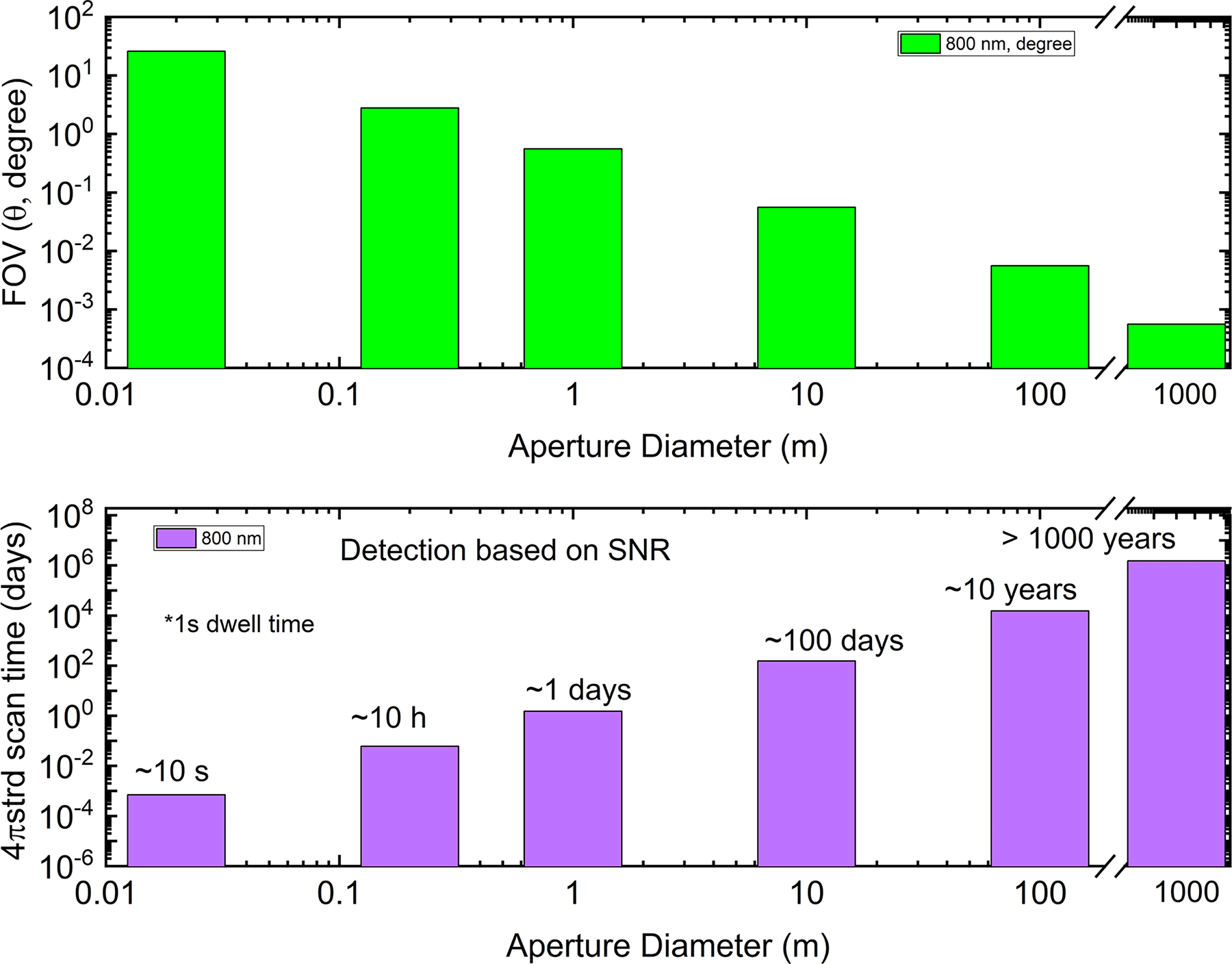
(Top) Field of view (FOV) as a function of aperture diameter for optical sensors operating at 800 nm. (Bottom) Scan time of the full 4π steradian volume versus aperture diameter. Smaller optical sensors had larger FOVs and faster scan times.

Fig. 6.

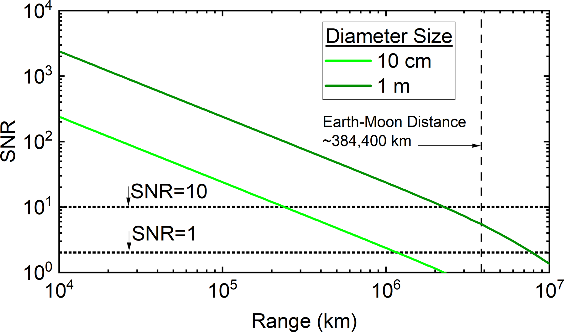
SNR versus operational range of a 10 cm and 1 m optical sensor operating at 800 nm. The figure shows that these more conventionally sized sensors could achieve detection for SNR ≥1 at ranges of ∼1.2 × 10⁶ km (diameter = 10 cm) and ∼8.1 × 10⁶ km (diameter = 1 m). SNR, signal-to-noise ratio.

Figure 7 shows the percentage of the Cislunar area that architectures comprised of small conventionally sized (D = 18.5 cm) optical sensors (operating at 800 nm wavelength) could detect the RSO. Together with Figure 5 (which plots the scan time), the results show that small optical sensors could scan the 4π sr volume at a range of 3.2 × 10⁶ km (SNR >6) in ∼10 h (where multiple sensors working in tandem reduced scan time linearly) and provided up to 65% detection coverage for the eight architectures studied. Figure 7 shows that a network of ∼10 small optical sensors was sufficient for providing a search and detection capability. However, note that no range information was provided from this type of architecture (just angle measurements), which was only partially sufficient for queuing other sensors for performing further detection and recognition. Therefore, we present the search and track capabilities provided by an active RF sensor architecture that could acquire accurate range information.

Fig. 7.

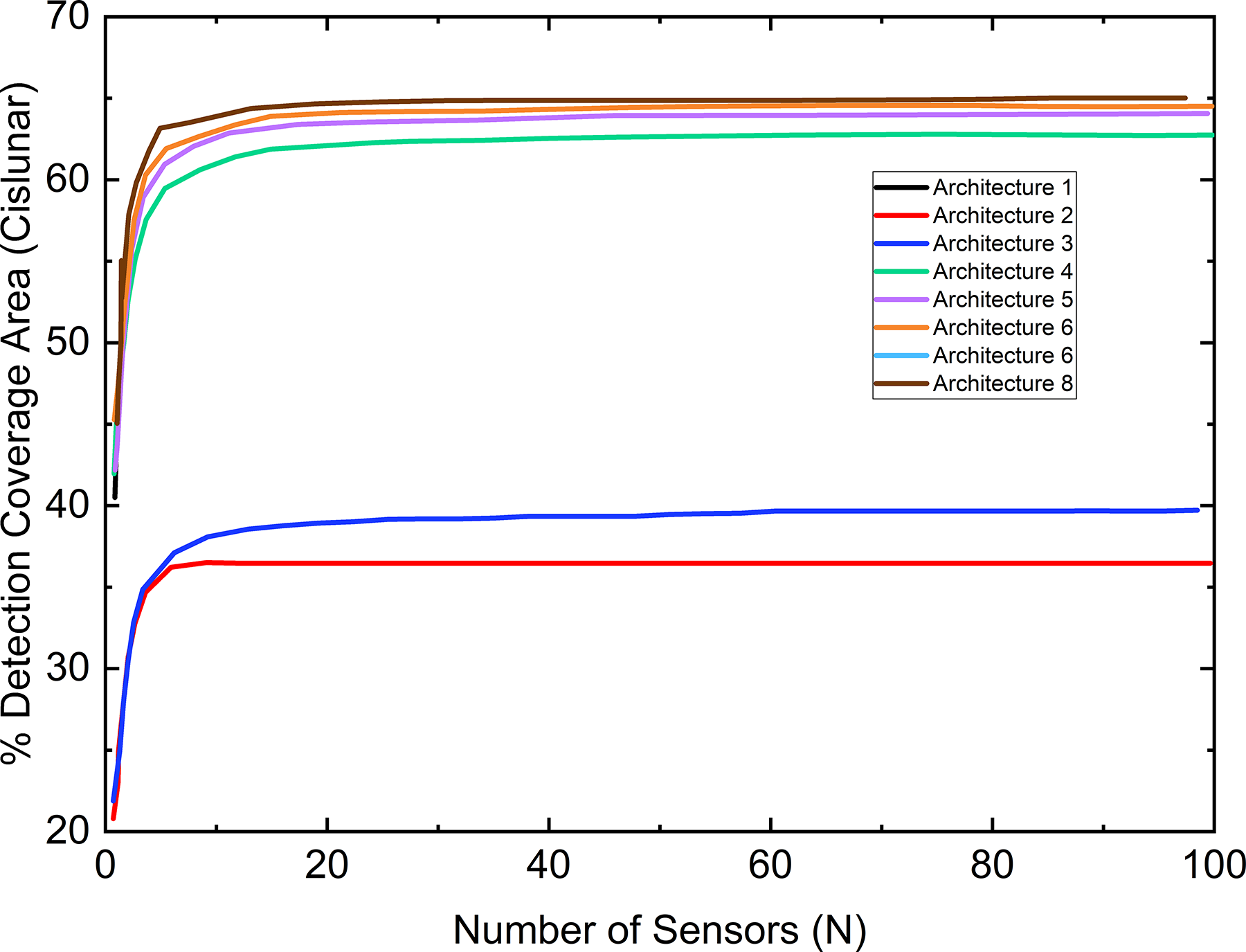
Results from the SSA analysis of architectures comprised of small (18.5 cm) optical sensors performing detection. The figure shows what percentage of the Cislunar area each architecture could detect as a function of sensor number. Note that the performance was averaged over 30 days, and the ability to detect was predicated on achieving an SNR ≥6.

Large active RF (search/detect and track)

Large active RF sensors were investigated for providing a search/detect and tracking capability within the Cislunar domain. The tracking performance was investigated by calculating the accuracy that an active RF sensor with an SNR ∼11.6 dB, a probability of detection of 95%, and a false alarm rate of 10⁻⁴ could measure an RSO with an RCS = 1 m².

Figure 8 details the search capability for the active RF sensors and platforms (consisting of eight RF sensors) by plotting the scan time to search the total 4π sr volume at a range of 100,000 km as a function of the RF aperture diameter and the RSO’s RCS. The figure shows a “V” shaped curve indicating that the optimization of the scan time of an active RF sensor was determined by multiple parameters, including (but not limited to) sensor diameter and RCS size. The full details of the radar range equation and calculation of the scan time are detailed in the Supplementary Data. A platform composed of eight active RF apertures with a diameter of ∼11 m could search for and detect an RCS of 7,854 m² with a scan time of 5.5 h (RCS of 1 m² takes 20 days with D = 100 m). These results indicated that large RF apertures were sufficient for monitoring common lanes of traffic in the Cislunar domain at a 95% probability of detection.

Fig. 8.

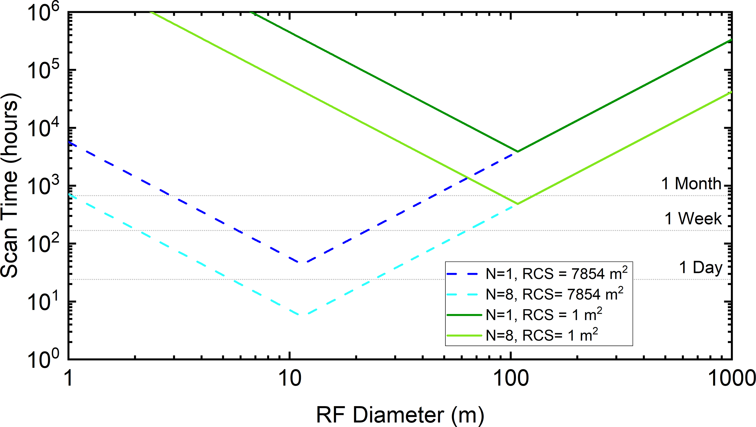
Scan time for the full 4π steradian volume at a range of 100,000 km versus diameter of active RF sensors modeled according to the parameters listed in Table 3. The performance of a single RF sensor (N = 1) and an RF platform comprising eight RF sensors (N = 8) is plotted for detecting an RSO with two different radar cross sections (RCS): 7,854 m² (corresponding to a cylindrical RSO with a height of 10 m) and 1 m² (comparable to small asteroids).

Next, the performance of how well a 100 m active RF sensor could track the RSO by calculating tracking accuracy was investigated. Accurate RSO tracking required measurements of the range to the RSO, its velocity, and angular position (see Supplementary Data). Figure 9 plots the degree of measurement accuracy as a function of the SNR. For reference, the Cramer–Rao limit was also plotted as a theoretical lower bound on the performance. The figure shows that with an SNR ∼11.6 dB, a 100 m active RF sensor could provide range measurement accuracy on the order of hundreds of meters over 100,000 km, velocity measurement accuracy on the order of 100 m/s, and angle measurement (monopulse radar configuration) accuracy on the order of 0.15 mrad. The positional uncertainty provided by large active RF sensors was superior to that provided by small optical sensors (which were on the order of ∼100 km). These results indicated that custody could be maintained 100% of the time, assuming continuous monitoring.

Fig. 9.

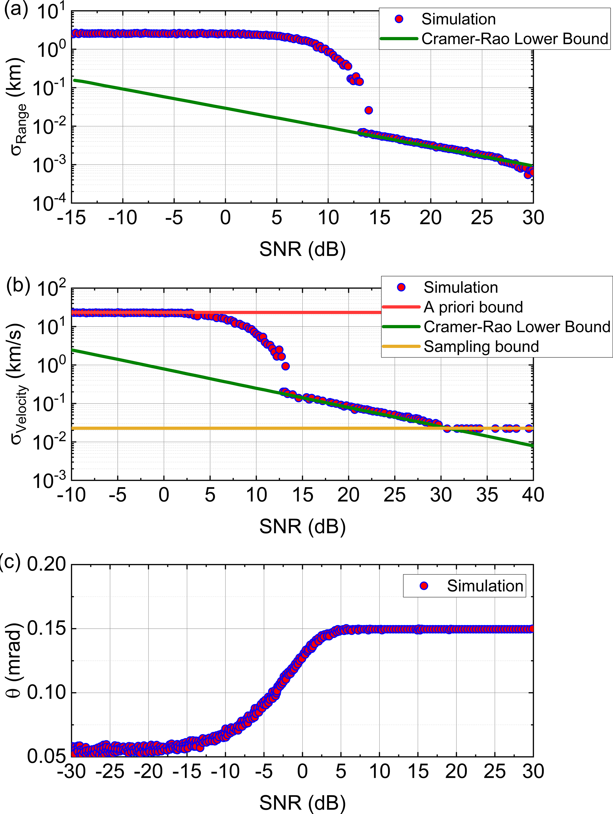
The level of accuracy that an active RF sensor (defined in Table 3) could obtain for measuring the (a) range, (b) velocity, and (c) angle to the RSO with an RCS = 1 m² as a function of SNR.

Cislunar SSA Performance

Large passive RF sensors (detection)

Figure 10(a–d) shows the data resulting from the CSSA performance analysis that placed passive RF sensors of varying diameters into eight Cislunar architectures (Table 7). The analysis considered the placement of a single passive RF sensor in each orbit and multiple sensors, up to a maximum of 50 sensors per orbit. The results show how much area coverage each architecture provided as a function of sensor number. The performance was measured as the percentage of the area where detection (SNR >1) occurred. The nominal number of sensors needed to achieve the optimal performance of architecture 8 is also plotted in each panel as a gray symbol. Architecture 8 was chosen because it contained the most orbits and generally had the best SSA performance. The optimal performance was defined as the minimum number of sensors required, where adding another sensor resulted in less than a 0.1% improvement in area coverage (i.e., when the performance curve derivative for architecture 8 falls <0.1). Figure 10 indicates that for each receiver aperture diameter (1, 10, 100, & 1,000 m), the detection performance generally improved with increasing sensor number; however, the number of sensors that led to the best performance depended on the sensor size. For example, for 1 m and 10 m diameter sensors, detection performance improved up to the addition of ∼18 sensors. However, for 100 m diameter sensors, performance did not improve beyond 13 sensors per orbit. This was tied to the increased operational range that a large-diameter sensor provided. Once enough sensors were placed into each orbit so that the operational range between one sensor overlapped with that of the nearest sensor, the performance was optimized so that the addition of more sensors did not impact the overall performance of the architecture.

Fig. 10.

(a–d) The coverage area and detection capability are analyzed as a function of sensor number for architectures consisting of passive RF sensors. Each panel in (a–d) represents the performance over a certain receiver diameter (D) size and contains a gray datapoint that is indicative of the number of sensors (per orbit) required to reach the optimized performance for architecture 8 (n₈). (e) The coverage area averaged over the performance of all sensor numbers is plotted as a function of sensor diameter for each architecture.

Fig. 11.

Max operational range that an optical sensor of varying wavelength (800 nm and 10 μm) could recognize the RSO according to the Johnson Criteria metric that required a minimum resolution of 0.77 m to achieve recognition.

Figure 10(e) shows the detection performance results averaged over all sensor numbers (n = 1–50). In total, smaller p-RF sensors offered some detection coverage (<20% of the Cislunar area); however, large apertures (D ≥1,000 m) were required to consistently provide coverage, where seven (D = 1,000 m) sensors placed in architecture 8 provided up to 93% coverage. Figure 10(e) also shows that architectures 1 and 6–8 provided the best coverage of the Cislunar area, where architecture 8 emerged in the highest coverage, at 93% of the area. Generally, architecture 8 exhibited the best performance, which was not surprising because it comprised the most orbits and therefore had the most overall sensors compared to the other architectures.

Large optical sensors (recognition)

Large optical sensors were assessed for providing a CSSA recognition capability. Note that for this investigation, recognition was dependent on using resolved imagery, driving the need for large sensors. There is the possibility of object recognition using unresolved imagery, which would relax sensor size constraints. Figure 11 plots the maximum operational range that large optical sensors could perform recognition, for two different wavelengths as a function of aperture size. The maximum operational range required that a sensor had a resolution of ≤0.77 m/pixel (resolution) and assumed perfect pointing (the sensor had been queued and oriented where to look to image the RSO). The figure shows that even with the factor of three blurring applied to the performance, a large VIS sensor was better suited for providing a recognition capability than a large LWIR optical sensor. The results from Figure 11 were used as inputs into the SSA modeling tool to define the optical sensor recognition performance.

Figure 12(a–d) shows the CSSA recognition performance results for all eight architectures comprised of optical sensors as a function of sensor number (n = 1–50) and sensor size (D = 1, 10, 100, & 1,000 m). Similar to Figure 10, the nominal number of sensors needed to achieve the optimal performance of architecture 8 is also plotted in each panel as a gray symbol using the same criteria previously described. Architectures comprised of small (D = 1–10 m) optical sensors resulted in a recognition capability <0.15% of the Cislunar area, even when the architectures contained hundreds of sensors. As aperture size increased, the SSA recognition performance also increased, and aperture diameters on the size scale of 1,000 m in diameter were required to provide recognition coverage >30%. Additionally, Figure 12 shows a similar trend to Figure 10, where the SSA performance generally increased with sensor number up to a limit. The limit (max number of sensors per orbit that improves performance) was tied to both the size of the sensors and the specific architecture. For small sensors (D = 1 m & 10 m), the more sensors the better because each sensor had such a small operational range that adding a new sensor typically provided added area coverage. For larger sensors (D = 100 m & 1,000 m), the addition of more sensors past ∼15 did not drastically improve performance because the operational range was long enough that the addition of another sensor only provided an overlap in coverage rather than additional coverage.

Fig. 12.

(a–d) The coverage area and recognition capability are analyzed as a function of sensor number for architectures consisting of optical sensors. Each panel in (a–d) represents the performance over a certain sensor diameter (D) size and contains a gray datapoint that is indicative of the number of sensors (per orbit) required to reach the optimized performance for architecture 8 (n₈). (e) The coverage area averaged over the performance of all sensor numbers is plotted as a function of sensor diameter for each architecture. The figure shows that very large optical apertures (D ≥1,000 m) were required to achieve >75%.

Figure 12(e) shows the results from the CSSA analysis, where the recognition performance was averaged over all sensor numbers. The figure shows how recognition coverage depended on optical sensor diameter and the number of sensors per orbit. Small apertures (1–10 m) provided negligible recognition capability, even with many sensors, while very large apertures (1,000 m) were required to achieve meaningful coverage (greater than 30%–70%). The results highlight that sensor size was far more critical than sensor number for enabling optical recognition performance across architectures.

DISCUSSION

Nominal CSSA Architecture

This section presents a representative architecture designed to enable accurate, persistent, and timely SSA within the Cislunar domain informed by the above results. Figure 13 illustrates a tiered system composed of multiple sensor types, each contributing unique capabilities.

At the foundation of this architecture are 10 small optical sensors (D = 18.5 cm) positioned in the Vulture Geocycler, L4 Planar, L2 Norther Halo, and L5 Planar Short Period orbits (total of 40 sensors). These provided a search capability with relatively fast scan times (∼10 h), covering approximately 65% of the Cislunar region. While limited in aperture size, these sensors offered faster area coverage in comparison to an active RF equivalent.

To augment detection capabilities, seven large passive RF sensors (D = 1,000 m) were positioned in the Vulture Geocycler orbit. These sensors extended detection coverage to ∼50% (which could be improved up to ∼92% if more sensors were placed in the L2, L4, and L5 orbits) of the Cislunar area, though their effectiveness was limited to RF-emitting RSOs (see parameters in Table 4).

For high-accuracy tracking, four active RF sensors (D = 100 m) were placed at equal distances along a 2.9× GEO orbit (refer to DeCoster et al.³ for detailed configuration). These sensors focused on key transit corridors between the Earth and Moon, offering tracking accuracies on the order of hundreds of meters over 100,000 km, with velocity measurements in the hundreds of m/s and angular resolution of approximately 0.15 mrad.

To support object recognition, a network of 45 large optical sensors (D = 100 m) were deployed across three periodic orbits around Earth–Moon Lagrange points L2, L4, and L5, with 15 sensors per orbit. These sensors achieved a recognition capability across ∼58% of the Cislunar domain, which could be enhanced to ∼75% coverage by adding similar sensors to the Vulture Geocycler orbit.

In summary, this nominal architecture delivered:

a search capability covering ∼65% of the Cislunar domain within a 10-h revisit cycle;

a detection capability over ∼50%–92% of the area via large passive RF sensors;

a recognition capability over ∼58%–75% of the domain through large optical sensors; and

a high-precision tracking capability enabled by strategically placed active RF sensors.

The tiered system relied on tipping and queuing, where small optical and passive RF sensors initiated detections, which were then followed up by large optical and active RF assets for further characterization and tracking.

Summary

This section provides a summary of the results to understand the relative importance of sensor type, size, and number on the CSSA performance for establishing a detection and recognition capability. First, an interpretation of the effect of sensor number and size on the CSSA performance is discussed, and then details from the machine learning approach used to extrapolate and generalize trends generated by the CSSA performance models are covered.

Figure 14 plots the minimum number of sensors needed to obtain the best measured performance for architecture 8 for both the passive RF and optical sensor results (gray datapoints in Figures 10 and 12). The figure illustrates that the optimal CSSA performance for both passive RF and optical sensors was more significantly enhanced by larger sensor diameters than by increasing the number of sensors. Figure 14(a) shows that a network of ∼18 (D = 1 m or 10 m) sensors per orbit provided a detection capability on the order of ∼4%–17% area coverage. Going beyond 18 sensors per orbit did little to improve performance. As the p-RF sensor size increased, fewer sensors were required to achieve the best measured performance, and the total area coverage also improved significantly, where >90% coverage was achieved with a few (<10) 1,000 m apertures. Next, Figure 14(b) shows that large optical apertures were a requirement for achieving a recognition capability in the Cislunar domain. Here, it was evident that a network of many small (D ≤10 m) optical sensors did very little to improve performance, which was limited to <0.002% area coverage. In fact, the addition of more than one sensor per orbit was negligible for improving the area coverage. Large (D ≥1,000 m) apertures were required to achieve a recognition capability over ∼75% of the Cislunar area of interest.

Fig. 13.

Illustration of a nominal CSSA architecture comprised of small and large optical and RF sensors to perform search, detection, recognition, and tracking of Cislunar objects. This architecture consisted of 10 (D = 18.5 cm) optical sensors (small blue circles) placed in the Vulture Geocycler, L4, L2, and L5 periodic orbits. The small optical sensors provided a fast (∼10 h) search and detection capability with moderate (∼65%) areal coverage. Seven (D = 1,000 m) passive RF sensors were placed in the Vulture Geocycler, which increased detection coverage of ∼50% of the area (but were limited to the detection of RF emitters). Four large (D = 100 m) active RF sensors were placed in a 2.9× GEO that provided high-accuracy tracking and overlapping coverage to monitor the region around the Earth (each individual sensor had a range of 100,000 km), and 15 (D = 1,000 m) optical sensors were placed in each periodic orbit (around L2, L4, and L5) and provided a recognition over ∼58% of the Cislunar area. The call-out box to the left shows how a tiered architecture of small and large optical and RF sensors would search, detect, track, and recognize an RSO in the Cislunar domain. GEO, geosynchronous orbit.

Fig. 14.

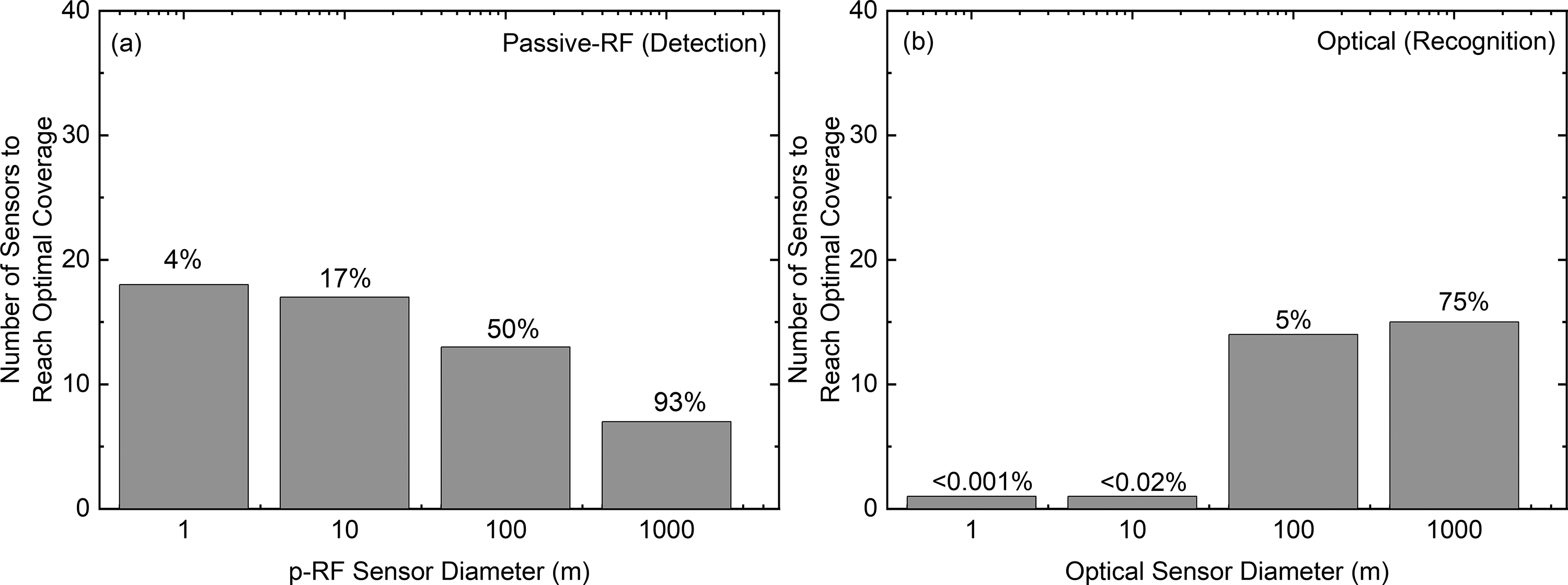
The minimum number of sensors (per orbit) required to achieve the best measured performance for architecture 8 comprised of (a) passive RF and (b) optical sensors as a function of sensor size. The data were adapted from the gray datapoints within each panel of Figures 10 and 12. The best measured performance was achieved when the addition of a sensor resulted in less than a 0.1% improvement in area coverage. The labels above each bar indicate the percentage of area coverage corresponding to optimal architecture performance.

Fig. 15.

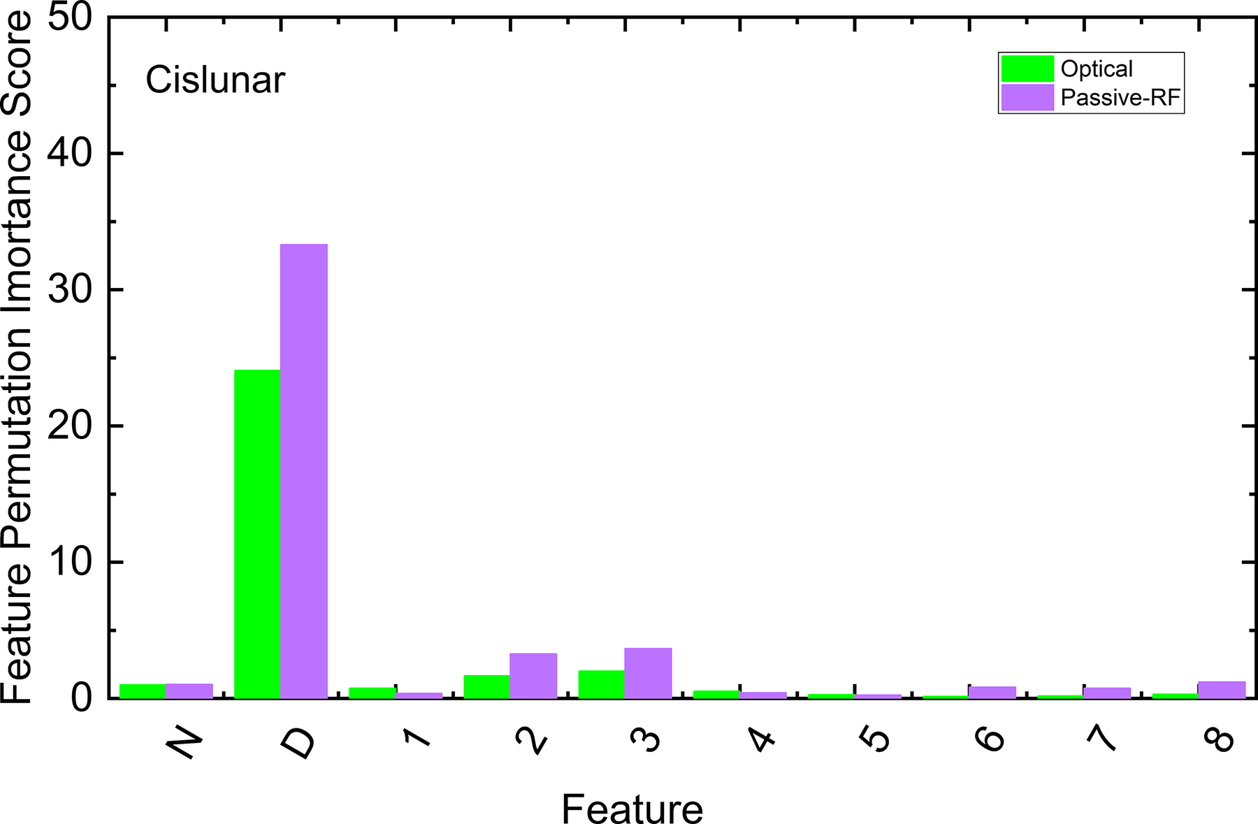
Feature permutation analysis applied to the machine learning (ML) results that detail the relative importance of certain SSA architecture features (sensor number (N), sensor diameter (D), and architecture number [1–8]) for predicting the performance of the CSSA parameter space toward detection (passive RF) and recognition (optical). The higher the permutation importance score, the more weight a certain feature has for predicting performance within the ML model.

Figure 14 should be interpreted as a performance envelope versus effective aperture (i.e., the aperture size used in the modeling that sets the image resolution, regardless of how that resolving power was achieved physically), not as a near-term assertion of access to contiguous 1,000 m apertures. The feasibility of access to large structures in space was motivated by maturing ISAM technologies such as those under development through DARPA’s NOM4D program. Projects like NOM4D may validate the materials and processes needed to build much larger structures in space beyond launch-fairing limits. These demonstrations would reduce risk in materials processing, autonomous assembly, and metrology, which are prerequisites for scaling to tens to hundreds of meters. Consistent with DARPA’s objective of enabling very large space structures, the 1,000 m end-members explored here represent a notional effective aperture used to bound recognition performance, while ∼10 m class apertures align with more near-term segmented/assembled approaches.

To understand the relative effects of CSSA parameters like sensor size, sensor number, and architecture type for predicting the performance of a CSSA architecture, a random forest machine learning model was trained on the data generated in Figures 10 and 12 to predict the performance of and extrapolate trends to other CSSA architectures (see section 2.4.2 for details). Figure 15 presents the feature permutation importance scores generated by the random forest machine learning model, trained to evaluate the impact of different variables on CSSA coverage. Feature permutation analysis assessed the relative importance of the CSSA architecture characteristics used to train the machine learning model, where a higher permutation importance score indicated that a particular feature was more significant for predicting the performance of the trained model. Sensor size (D) emerged as the most influential feature, indicating that the sensor size was the most important feature for predicting CSSA detection/recognition coverage. The figure also indicates that sensor size (D) had a slightly greater effect for passive RF sensors than optical sensors. This was likely due to the trend uncovered in Figure 14, which showed that smaller p-RF sensors provided some detection coverage, whereas small optical sensors did not provide any significant recognition capability. Additionally, passive RF sensors were less limited by non-optimal viewing conditions, like exclusion zones, which could play a role in the results. Figure 15 also indicates that sensor number (N) and architecture number had roughly the same level of importance for predicting CSSA architecture performance.

CONCLUSIONS

This study investigated how access to large (D ≥100 m) optical and RF sensors through technology maturation in ISAM materials and designs could impact future space operations by enabling a persistent, accurate, and timely Cislunar SSA capability. The results indicated that CSSA architectures comprised of large 100 m diameter active RF sensors positioned into strategic orbits could provide a Cislunar search/detection capability, with a scan time of 5.5 h (RCS = 7,854 m²)-20 days (RCS = 1 m²) that could be further reduced linearly by adding more RF sensors to the architecture. Additionally, a large active RF sensor provided high-quality tracking in range (accuracy on the order of ∼100 m over ∼100,000 km), velocity (accuracies on the order of 100 m/s), and angle measurements (accuracies on the order of 0.15 mrad), so that custody of Cislunar RSOs could be maintained 100% of the time. Next, it was shown that large (D ≥100 m) passive RF sensors were well suited for providing detection over the Cislunar area. Specifically, architectures comprised of 100 m sensors could cover as much as 50% of the Cislunar area, and architectures comprised of 1,000 m sensors could cover as much as 93% of the Cislunar area. Furthermore, large optical sensors (D = 1,000 m) were a requirement for enabling a resolution-dependent recognition capability over as much as 75% of the Cislunar domain. Additionally, sensor size, rather than sensor number or architecture type, emerged as the most important parameter for predicting CSSA area coverage performance.

AUTHORS’ CONTRIBUTIONS

M.E.D.: Conceptualization, methodology, formal analysis, data curation, and writing—original draft. R.A.: Formal analysis (RF) and data curation. A.G.: Formal analysis (orbit design and modeling). D.B.: Formal analysis (optical) and data curation. S.P.: Formal analysis (RF). A.N.: Formal analysis (ML). M.T.: Conceptualization and writing—review and editing.

Footnotes

FUNDING INFORMATION

This material is based upon work supported by the Defense Advanced Research Projects Agency under Contract No. HR0011-22-D-0001/Task Order HR001123F0002.

DISCLAIMER

The views and conclusions contained in this article are those of the author and should not be interpreted as representing the official policies, either expressly or implied, of the Defense Advanced Research Projects Agency or the U.S. Government. During the preparation of this work, the authors used ChatGPT 4o in order to improve the readability and language of the introduction. After using this tool/service, the authors reviewed and edited the content as needed and take full responsibility for the content of the publication.

AUTHOR DISCLOSURE STATEMENTS

The authors declare that they have no known competing financial interests or personal relationships that could have appeared to influence the work reported in this article.

Supplemental Material

References

Kelso

. Analysis of the Iridium 33-Cosmos 2251 Collision. In Maui, HI; 2009.

The White House [Internet]. 2022 [cited 2024 Sep 26]. FACT SHEET: First National Cislunar Science & Technology Strategy | OSTP.

DeCoster

, Awadallah

, Blodgett

, et al. On-orbit assembly and manufacturing of large structures to enable space situational awareness. In: AIAA SCITECH 2023 Forum. American Institute of Aeronautics and Astronautics; 2023; doi: 10.2514/6.2023-1118

Fowler

, Paley

. Observability metrics for space-based cislunar domain awareness. J Astronaut Sci, 2023; 70(2):10.

Koblick

, Choi

. Cislunar orbit determination benefits of moon-based sensors. In Maui, HI; 2022. p. 12.

Badura

, Shimane

, Gregoire

, et al. System design and analysis for cislunar space domain awareness through distributed sensors. In: AAS/AIAA Astrodynamics Specialist Conference, Charlotte, NC. 2022. pp. 1–20.

Frueh

, Howell

, DeMars

, Bhadauria

. Cislunar space situational awareness. In: 31st AIAA/AAS Space Flight Mechanics Meeting, 2021. pp. 6–7.

Frueh

, Little

, McGraw

. Optical sensor model and its effects on the design of sensor networks and tracking. In: Advanced Maui Optical and Space Surveillance Technologies Conference (AMOS). 2019.

Baker-McEvilly

, Bhadauria

, Canales

, Frueh

. A comprehensive review on Cislunar expansion and space domain awareness. Prog Aerosp Sci, 2024; 147:101019.

10.

Cui

, Zhang

, Gao

, et al. Radio frequency identification and sensing techniques and their applications—A review of the State-of-the-art. Sensors (Basel), 2019; 19(18):4012.

11.

Peric

, Livada

., Technical, Technological and Application Limitations of the Electro-Optical Surveillance Systems. In Belgrade, Serbia; 2018. pp. 276–281.

12.

Sjaardema

, Smith

, Birch

. History and Evolution of the Johnson Criteria. 2015 p. SAND2015–6368, 1222446, 606152. Report No.: SAND2015–6368, 1222446, 606152.

13.

Chung

. C166. The radar cross section of known low observable satellite shape. 2013.

14.

Mahafza

. Radar Systems Analysis and Design Using MATLAB. 3rd ed. FL: CRC Press; 2012.

15.

Cheng

, Rivkin

, Michel

, et al. AIDA DART asteroid deflection test: Planetary defense and science objectives. Planet Space Sci, 2018; 157:104–115.

16.

Richards

. Fundamentals of Radar Signal Processing. 3rd ed.. NY: McGraw Hill; 2022.

17.

Ram

, Singh

, Ghatak

. Optimization of radar parameters for maximum detection probability under generalized discrete clutter conditions using stochastic geometry. IEEE Open J Signal Process, 2021; 2:571–585.

18.

Couch

. Digital & Analog Communication Systems. 8th edition. Upper Saddle River, NJ: Pearson; 2012. 792 p.

19.

Shihabi

. Iris V2.2 SmallSat Deep Space Transponder. Pasadena, CA: National Aeronautics and Space Administration Jet Propulsion Laboratory.

20.

Cohen

. Lunar Flashlight Mapping Lunar Surface Volatiles Using a CubeSat. FISO Telecon; 2015.

21.

Bokulic

, Flaherty

, Jensen

, McKnight

. The NEAR spacecraft RF telecommunications system. JHUAPL Tech Dig, 1998; 19(2):213–219.

22.

Holzinger

, Garretson

. A Primer on Cislunar Space. Air Force Research Laboratory; 2021 p. 23. Report No.: AFRL 2021-1271.

23.

Schaub

, Junkins

. Analytical Mechanics of Space Systems, Second Edition. 4th ed. Reston, VA: AIAA Educational Series; 2018. https://arc.aiaa.org/doi/book/10.2514/4.867231

24.

Gurfil

, Seidelmann

. Celestial Mechanics and Astrodynamics: Theory and Practice. Springer; 2016.

25.

Roy

. Orbital Motion. 4th ed. Boca Raton: CRC Press; 2020. 544 p.

26.

Howell

. Three-dimensional, periodic, ‘halo’ orbits. Celest Mech, 1984; 32(1):53–71.

27.

Farquhar

. The utilization of halo orbits in advanced lunar operations. The utilization of halo orbits in advanced lunar operations/by Robert W. Farquhar. Washington. 1971.

28.

Gómez

, Koon

, Lo

, et al. Connecting orbits and invariant manifolds in the spatial restricted three-body problem. Nonlinearity, 2004; 17(5):1571–1606.

29.

Folta

, Pavlak

, Haapala

, et al. Earth–Moon libration point orbit station keeping: Theory, modeling, and operations. Acta Astronaut, 2014; 94(1):421–433.

30.

Szebehely

. Description of the Restricted Problem. In: Theory of Orbit. Elsevier; 1967. pp. 7–41.

31.

Acton

. Ancillary data services of NASA’s navigation and ancillary information facility. Planet Space Sci, 1996; 44(1):65–70.

32.

Acton

, Bachman

, Semenov

, Wright

. A look towards the future in the handling of space science mission geometry. Planet Space Sci, 2018; 150:9–12.

33.

Breiman

. Random forests. Mach Learn, 2001; 45(1):5–32.

34.

Pedregosa

, Varoquaux

, Gramfort

, et al. Scikit-learn: Machine learning in Python. J Mach Learn Res, 2011; 12(85):2825–2830.

35.

Puga

, Krzywinski

, Altman

. Bayesian networks. Nat Methods, 2015; 12(9):799–800.