Sage Journals: Discover world-class research

Abstract

Disaggregating depression into stable trait-like and fluctuating state-like components provides insights into potential mechanisms underlying depression; predictors of these components can point to potentially tractable risk factors for depression onset. Using latent-trait-occasion modeling, we extracted state- and trait-depression components from the Short Mood and Feelings Questionnaire obtained in young people ages 11 to 26 from a population-based study in England (Avon Longitudinal Study of Parents and Children; N = 7,364). The proportion of state variance ranged from 91.9% (age 11) to 36.8% (age 26), decreasing during adolescence and stabilizing from age 22. The proportion of trait variance increased correspondingly. Female sex correlated with trait variance and with state variance only during adolescence (ages 12–19). Life events, school enjoyment, maternal depression, and parent–child relationship quality predicted state variance during adolescence, whereas anxiety was the main predictor during emerging adulthood. The greater role of state factors in early adolescence suggests that depression is more modifiable at younger ages.

Keywords

latent-trait-occasion modeling time-varying variance depression adolescence psychological development Avon Longitudinal Study of Parents and Children

Depression constitutes one of the greatest causes of disability worldwide, exerting one of the highest disease burdens globally of all physical and mental disorders (Q. Liu et al., 2020). A recent meta-analysis across 29 countries (N = 528,293 participants) indicates a prevalence of 21.3% for mild to severe depression in children and adolescents ages ≤ 18 years (Lu et al., 2024). To best inform early intervention strategies, it is critical to understand depressive symptoms during sensitive developmental phases (Schubert et al., 2017; Thapar et al., 2022). Epidemiological studies indicate that depressive-symptom incidence increases from childhood to adolescence and then decreases and stabilizes in young adulthood (Shore et al., 2018; Solmi et al., 2022). Depressive disorder, representing a more severe manifestation of depressive symptoms, is relatively rare before adolescence and then increases in incidence until peaking around age 20 (Solmi et al., 2022). This developmental period of adolescence is characterized by ongoing psychobiological changes and major life events (Dahl et al., 2018; Sawyer et al., 2018). For prevention efforts, developmental dynamics of depression and any associated risk or protective factors need to be precisely understood (Thapar et al., 2022). Although previous studies investigated changes in mean levels of depressive symptoms and identified distinct symptom trajectories during these transitional phases (for a review, see Schubert et al., 2017; Weavers et al., 2021), little is known about the stability of the variance in depressive symptoms developmentally (Prenoveau, 2016).

Understanding the stability of depression is important because depression exhibits patterns of both persistence and fluctuation (Polanczyk et al., 2015; Solmi et al., 2022; Thapar et al., 2022). Some individuals show chronic or recurrent symptoms over many years, whereas others experience substantial changes in depressive mood in response to life circumstances (Herrman et al., 2022; LeMoult et al., 2020). There are two common ways to quantify stability across individuals over time: (a) the intraclass correlation coefficient (ICC), which quantifies the ratio of between-persons variance to total variance (range = 0–1) and high ICC indicating high between-persons stability, and (b) rank-order stability, which assesses the degree to which individuals maintain their relative standing on depression across time. High rank-order correlations indicate that people who are more depressed than others at one time point tend to remain more depressed later, reflecting consistency in individual differences over time. These approaches have revealed low to moderate depression stability in childhood and adolescence. For example, Morken et al. (2021) found low to moderate depression rank-order stability from ages 4 to 14 (between ages 4 and 6: r = .17; between ages 12 and 14: r = .55), increasing between ages 12 and 14, and an average ICC of .22 for major depressive disorder. Mason et al. (2017) reported a similar increasing pattern across ages 11, 18, and 21. Yet neither of these approaches disentangle between-persons individual differences from within-persons fluctuations, as is accomplished using within-between models of panel data, such as the random intercept cross-lagged panel model (RI-CLPM; Hamaker, 2023). In within-between models, between-persons variance represents differences across individuals’ overall depressive symptoms estimated over multiple time points, informing how people differ from one another on average. Within-persons variance captures how an individual’s depressive symptoms fluctuate around the individual’s own mean over time. RI-CLPMs are typically used to examine reciprocal between- and within-persons relationships between two variables over time, such as depression and self-esteem during adolescence (Masselink et al., 2018).

The latent-state-trait-occasion (LSO) model is a multiple-indicator version of a within-between model (Usami et al., 2019), which can be used to model stability of a single construct across developmental periods (Prenoveau, 2016). Multiple depressive symptoms form each latent state-depression construct at each wave (Fig. 1), and from these factors, the individuals’ latent-trait (between-persons time-invariant) and latent-occasion (time-varying) components of depression can be disaggregated. These components will be subsequently referred to as “trait depression” and “state depression,” respectively. This approach provides a formal estimate of the proportion of reliable variance that is stable (trait-like) across the measured waves versus situationally variable (state-like) and allows researchers to examine how these proportions change over time (Cole et al., 2005).

Fig. 1.

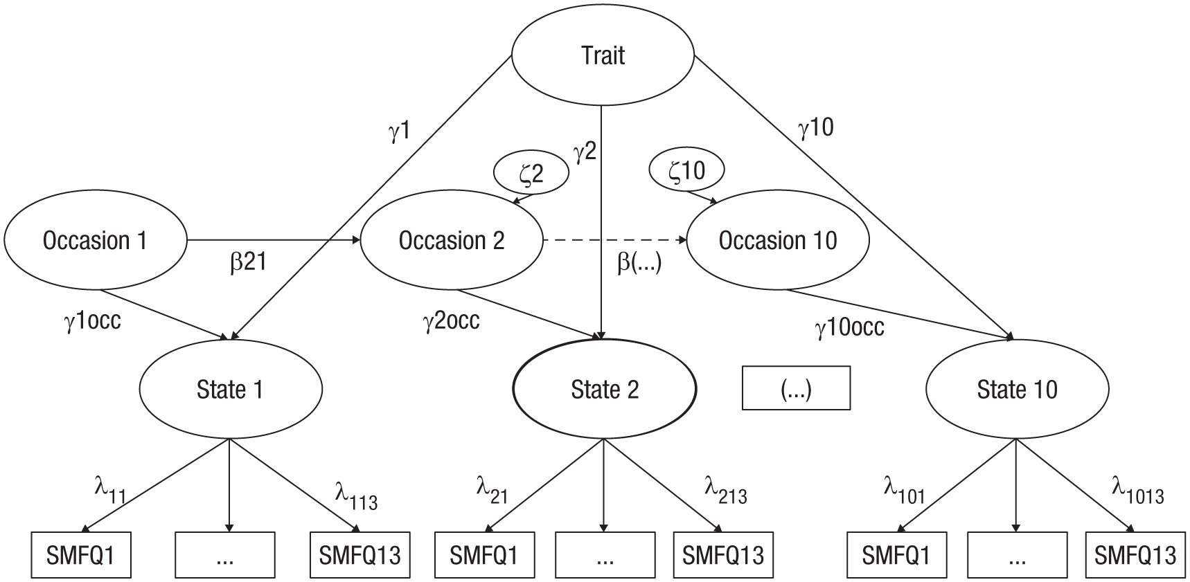
Illustration of the latent-state-trait-occasion model of the Short Mood and Feelings Questionnaire. State = state factor; Occasion 1–10 = occasion factors; γ = trait factor loading; γ_occ = occasion factor loading; ζ = occasion-specific latent residual variance; λ = factor loadings; β = autoregressive pathway between occasions. For reasons of space, this model is illustrated for only three occasions and three indicator variables.

Interpreting the relative contributions of state and trait variance over development may inform depression theories and research (Köhler et al., 2019). A predominance of trait variance would suggest that depressive symptoms largely reflect stable individual differences, consistent with models emphasizing enduring vulnerabilities (e.g., cognitive schemas, personality traits, biological predispositions; Hölzel et al., 2011). In contrast, greater state variance would imply that depressive symptoms present a more dynamic system, sensitive to environmental context (Hammen, 2016), stress exposure (LeMoult et al., 2020), or feedback loops (Wittenborn et al., 2016). Note that if trait variance increases over time, this could indicate that depressive symptoms are becoming more entrenched during development, potentially pointing to chronicity, entrenchment, or scar effects (in which prior depression symptoms create lasting cognitive or biological changes; Klein et al., 2011; Rohde et al., 1991, 1994; Schlechter et al., 2024). State variance increasing over time could indicate the increasing importance of the adolescents’ changing environment in contributing to depressive symptoms (Jenness et al., 2019; Vidal Bustamante et al., 2020).

In previous LSO research, only moderate levels of variance were explained by the latent-trait component of depression in children (Cole et al., 2017) and adolescents (Holsen et al., 2000; Wu, 2016). Across studies from children and adolescents ages 7 to 17, trait factors explained between 31% and 63.4% of the variance in participants who were followed up for 3 to 4 years (Cole et al., 2017; LaGrange et al., 2011; Prenoveau et al., 2011; Wu, 2016). Thus, a notable degree of variance in these studies was explained by state components, which is likely due to the myriad of social and psychobiological changes taking place during development (Joinson et al., 2012) or the potential influence of life events in key developmental periods (Korten et al., 2012). These developmental changes continue into emerging adulthood (Arnett, 2000; Whitaker et al., 2016), yet the importance of state and trait depression during the transition from adolescence into emergent adulthood remains untested. Given the importance of adolescence for emergent psychopathology (Dahl et al., 2018) and the long-lasting impact of early onset depression on future outcomes (Rohde et al., 2013), it is important to investigate state and trait components of depression in a broader developmental period than previously studied (note that childhood is defined as ages 6–10; adolescence is defined as 11–18, yet it is sometimes argued that it may extend to 24; and emerging adulthood is defined as 19–26; Arnett, 2000; Sawyer et al., 2018). Considering a longer time frame of observation into emerging adulthood is critical because variance that appears stable over a short period may fluctuate over longer intervals (Hamaker, 2023). If a study spans only a few years of development, some variance in depression may appear trait-like. Yet with an increased time frame, there may be shifts in variance because of developmental, social, or environmental changes (Dahl et al., 2018; Sawyer et al., 2018), revealing previously hidden state variance, which has important theoretical and practical implications.

Importantly, after disentangling these components of depression in the LSO model, predictors of the trait factor and of the different state factors can be investigated (Prenoveau, 2016). State factors represent the part of depression that is changing over time, which by merit of reflecting less entrenched symptoms, is more likely to constitute an amenable intervention target. Examining predictors of the state factors thereby enables us to pinpoint the developmental timing of risk factors that predict the changing aspect of depression at a developmental period when depression often manifests and can lead to lifelong persistent and severe depression (Thapar et al., 2022). The trait factor captures the stable, enduring component of depression, reflecting persistent individual differences that are less influenced by situational changes (Prenoveau, 2016). Although trait-like variance is stable over longer periods and so less likely to naturally change over development, identifying its predictors provides relevant insights into early risk factors for longer-term vulnerabilities. These risk factors can be particularly targeted in preventive strategies and early interventions to reduce the likelihood of chronic-depression trajectories. Table 1 depicts our hypotheses regarding important predictors and whether they are related to time-invariant and time-varying variance of the depression construct across development. These predictors include the effects of sex (Patalay & Fitzsimons, 2018), temperament (Elovainio et al., 2015), maternal depression (S. H. Goodman et al., 2011), parenting (Yap et al., 2014), stressful life events (Korten et al., 2012), childhood trauma (McLaughlin et al., 2012), school climate (Ford et al., 2021), and former mental-health problems (St. Clair et al., 2017). Although associations of these predictors and their developmental timing with depressive symptoms are well established (Thapar et al., 2022), this has yet to be examined in the context of state factors of depressive symptoms that have been disaggregated from trait factors (Prenoveau, 2016).

Table 1.

Hypotheses Regarding the Tested Constructs and Their Association With Time-Invariant and Time-Varying Variance in Depression and Assessment

Predictor	Time-invariant variance	Time-varying variance	Assessment in the current study
Sex	• Stable depression prevalence differences across gender with a ratio around 2:1 for women compared with men (Salk et al., 2017)	• Puberty may affect males and females differently (Lewis et al., 2018); gender differences emerge around ages of 12 to 15 (Patalay & Fitzsimons, 2018).	• Dichotomous male/female assessment at baseline during the ALSPAC study/based on biological sex
Temperament and child’s problems	• Relatively stable across time and context and consistently related to depression (Bould et al., 2013; Elovainio et al., 2015)	—	• Temperament at 57 months: mother reports; Emotionality, Activity, and Sociability Temperament Scale; 5-point scale from (1) not characteristic pf your child to (5) very characteristic of your child (Buss & Plomin, 1984) • Strength and Difficulties Questionnaire completed by mothers for their children at age 7 (R. Goodman, 2001); 25 questions, five subscales; we used the total difficulties score.
Maternal depression	• Associated with children’s general vulnerability to psychopathology pointing to stable factors in families (meta-analysis; S. H. Goodman et al., 2011)	—	• One question when child was age 11 whether mother has had or continued to have depression since the child’s fifth birthday (yes and consulted doctor, yes but did not consult doctor, and no)
Quality of parent–child relationship Conflict with parents		• May be especially relevant during sensitive periods in early adolescence, when adolescents need to feel understood and supported (Yap et al., 2014).	• Relationship with parents at age 14: four child-reported items on the closeness of the parent–child relationship at age of 14 (how often the child tells the parents about their friends); responses from (1) almost always to (5) never; α = .87; items were recoded so that high scores reflect a closer relationship.• Mother–child conflict age 7: assessed with mother-reported frequency with which mother has battle of wills with child on a scale from (1) never to (4) frequently.
Stressful life events/childhood trauma	• Associated with onset of internalizing symptoms (McLaughlin et al., 2012) and depression in adolescence (Korten et al., 2012)• Around one-third of mental-health problems are attributable to childhood adversity (Kessler et al., 2010).	• Recency effects indicate that childhood adversity has most profound impact following its occurrence (Dunn et al., 2018).	• Life events since age 12 were assessed when participants were 16 years old: list containing 22 events (e.g., “death of a close friend,” yes/no).• Traumatic experiences perpetrated by an adult responsible for the child’s care were reported retrospectively at age 22 for childhood (before age 11) and adolescence (ages 11–17). Frequency of events, such as domestic violence, physical abuse, and emotional neglect, were indicated on scale from (1) never to (5) very often.
School enjoyment and school achievement	• Schools alone account for a small variation in psychopathology (Ford et al., 2021).	• School enjoyment is related to internalizing symptoms (Finning et al., 2019).• Meta-analysis of longitudinal studies: weak correlation of school ability with depression (Huang, 2015) and association higher in younger adolescents	• School ability age 10: assessed with one question, whether the child is good at all school subjects on a scale from (1) not true to (5) true • School enjoyment at ages 11 and 14: one question of whether the child’s school is a place where the child really likes to go each day; scale with options (1) agree to (4) disagree
Anxiety symptoms	• Transdiagnostic perspectives suggest shared liability (St. Clair et al., 2017).	• Anxiety symptoms tend to increase the vulnerability for depression (Kessler et al., 2010; Merikangas et al., 2010).	• Anxiety age 22: Generalized Anxiety Disorder Scale: well-validated self-report anxiety scale with seven items (Löwe et al., 2008); 4-point scale from 1 (not at all) to 4 (nearly every day), $ω_{t}$ = .93, α = .91.
Psychotic symptoms	• Depressive and psychotic symptoms were represented by p-factor (Stochl et al., 2015).	• Residual symptoms may precede depressive-symptom development (Keenan et al., 2009; Kessler et al., 2010; Merikangas et al., 2010).	• Psychotic symptoms age 17: psychosis-like symptoms questionnaire (Horwood et al., 2008); eight questions, for example, receiving messages or hearing voices; response options: (1) no, never; (2) yes, maybe; (3) yes, definitely (α = .71)
Self-rated health	• Self-rated health is a predictor for long-term prognosis of depression (Ambresin et al., 2014).	• Decreases in health may account for transient depressive symptoms (Ambresin et al., 2014; Merikangas et al., 2010).	• General health: one question on self-reported general health on 5-point Likert-type rating scale from 1 (excellent) to 5 (poor) at the ages 19, 21, and 22 years

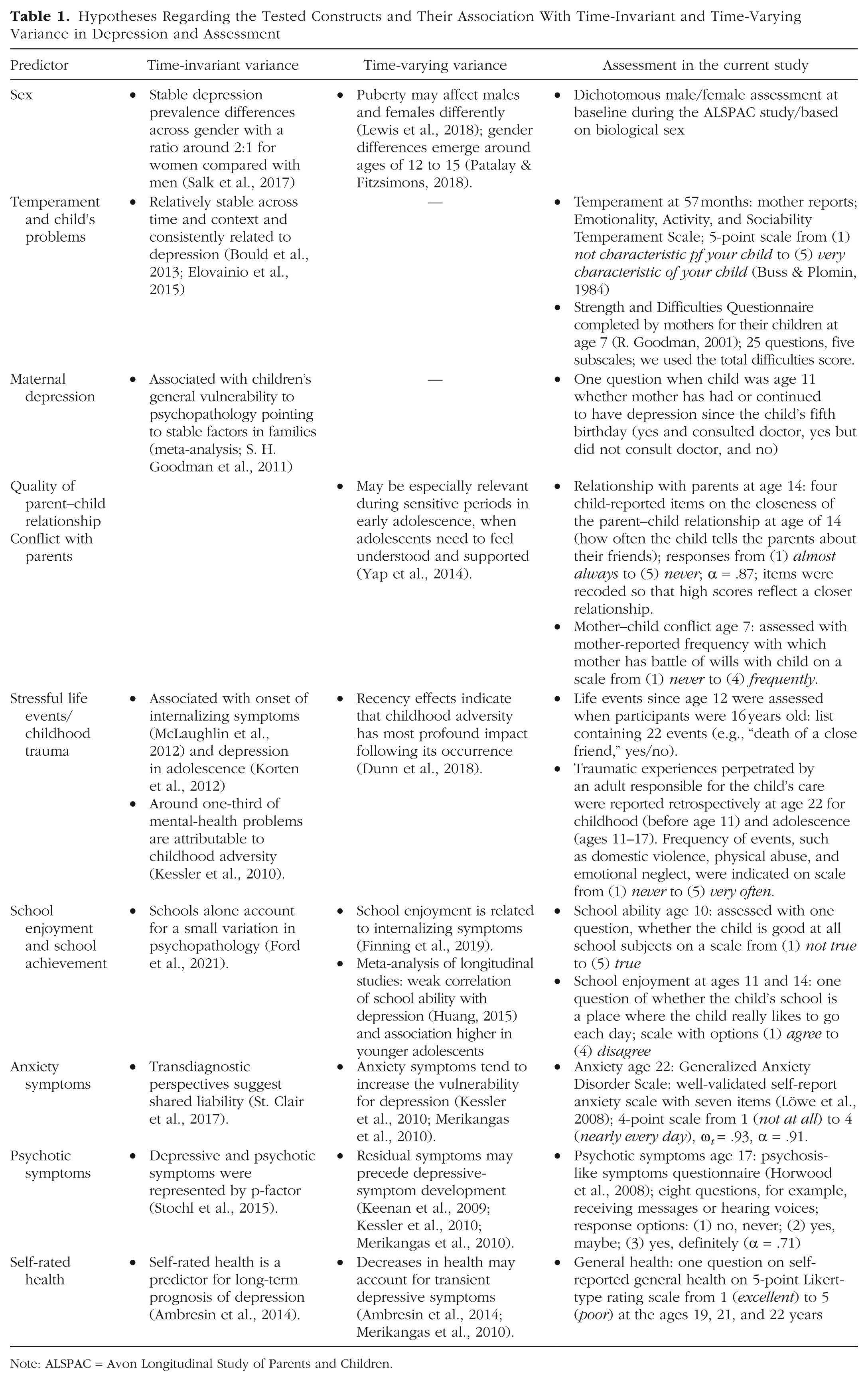
Note: ALSPAC = Avon Longitudinal Study of Parents and Children.

Beyond the relative contribution of individual predictors to trait and state factors of depression, it is also important to consider potential interactions between predictors that may influence state depression around the time of its occurrence. First, Maternal Depression × School-Related Variables may be relevant because higher maternal depressive symptoms could reduce parental support and thereby exacerbate school difficulties, increasing state depressive symptoms (Ford et al., 2021; S. H. Goodman et al., 2011). Second, Parent–Child Relationship Quality or Conflict × Early Temperament interactions may influence state depression because the effects of early temperament traits on depression can be buffered or amplified by the quality of familial relationships (Bould et al., 2013; Elovainio et al., 2015; Yap et al., 2014). Third, Life Stressors (Life Events and Trauma) × Mental-Health Problems may predict state depression, consistent with diathesis-stress models in which early vulnerability heightens sensitivity to later stressors (Korten et al., 2012; St. Clair et al., 2017). Examining such moderation models during specific developmental periods can inform mechanistic studies on the interplay of child, parent, and contextual factors, providing insight into the processes that contribute to depressive episodes.

The Present Research

In the present study, we (a) aimed to investigate the contribution of trait and state factors to depression from ages 11 to 26 by drawing on data from the Avon Longitudinal Study of Parents and Children (ALSPAC), a population-based study in southwest England. We hypothesized that the state variance components would be more pronounced at younger ages and gradually decrease and stabilize during emerging adulthood, as developmental change slows down (Dahl et al., 2018; Thapar et al., 2022). We then (b) examined how established predictors of depression (e.g., sex, school variables, parenting, life events, and previous mental-health problems) relate to the state and trait components of depressive symptoms. In addition, we tested selected moderation models to discern potential interaction effects on state depression.

Method

Transparency and openness

Preregistration

This study was not preregistered.

Data, materials, code, and online resources

Data cannot be shared because of the ALSPAC data policy. The study website contains details of the data that are available through a fully searchable data dictionary and variable search tool (http://www.bristol.ac.uk/alspac/researchers/our-data). The R Code including markdowns for html outputs is available on OSF: https://osf.io/9hyve/?view_only=c25856c0cfaf4139beb0927b78e2efe3.

Reporting

We report how we determined our sample size, all data exclusions, all manipulations, and all measures in the study.

Ethical approval

The ALSPAC Law and Ethics Committee and Local Research Ethic Committee gave ethical approval for the study. Informed consent for the use of data collected via questionnaires and clinics was obtained from participants following the recommendations of the ALSPAC Ethics and Law Committee at the time.

ALSPAC

ALSPAC is a population-based study in southwest England. From April 1, 1991, to December 31, 1992, 14,541 pregnant mothers and their children were enrolled in the study and then assessed throughout their lives (Boyd et al., 2013; Fraser et al., 2013; Northstone et al., 2019). Of these participants, 13,988 were alive at 1 year of age. At age 7, the sample was refreshed, which resulted in a final sample of N = 15,447 pregnancies, which resulted in a final sample of N = 14,901 participants. Compared with the UK population, ALSPAC participants were more likely to have higher education and be White and were less likely to receive free school meals (Boyd et al., 2013). Full cohort-profile descriptions are also available (Boyd et al., 2013). The Short Mood and Feelings Questionnaire (SMFQ) was used to assess depression at 10 time points from early adolescence to young adulthood, ranging from 11 to 26 years of age. For demographic characteristics for participants at these 10 time points, including sex, ethnicity, maternal qualification, and financial difficulties reported by mothers, see Table S1 in the Supplemental Material available online. Study data were collected and managed using REDCap (Research Electronic Data Capture) electronic-data-capture tools hosted at the University of Bristol (Harris et al., 2009).

Measures

Depressive symptoms were assessed with the 13-item Short Mood and Feelings Questionnaire (SMFQ; Angold et al., 1995). Participants indicated depressive symptoms from the last 2 weeks with the response categories not true (0), sometimes, (1) and true (2), leading to scores from 0 to 26. The SMFQ has good reliability and validity and is meant as a screening instrument designed for children and adolescents (Turner et al., 2014). Overall psychometric evidence indicates that the SMFQ can be used to measure the same construct over time. Specifically, in ALSPAC, we have demonstrated strict longitudinal measurement invariance in SMFQ from ages 14 to 26; evidence is weaker when this model included ages 11 to 13 (i.e., Δ root mean square error of approximation [RMSEA] supported scalar invariance, but Δ comparative fit index [CFI] did not, yet the overall scalar and strict invariance model fit remained good; Schlechter, Wilkinson, et al., 2023). Measurement details of the predictor variables are summarized in Table 1.

Analysis strategy

Missingness

All analyses were conducted in R (Version 4.01; R Core Team, 2021) using the lavaan package (Rosseel, 2012) for the latent-state-trait models. Data were treated as missing at random (MAR), in line with former reports that identified being male, having mothers with poorer educational attainment, and having a younger mother as factors that were associated with missingness in this sample (Kwong, 2019). Moreover, SMFQ scores at Wave 1 predicted missingness and a range of other variables that we report in Table S2 in the Supplemental Material, supporting our MAR assumption. The highest level of missingness compared with Wave 1 was 55% (3,305 / 7,364) at Wave 7.

Data were treated as ordinal because the SMFQ has three response options. Thus, we used the weighted least squares mean and variance (WLSMV) adjusted estimator for all models (Asparouhov & Muthén, 2010). Simulation studies have shown that parameter and standard-error estimates from WLSMV remain relatively unbiased even with high levels of missingness when the sample size is sufficiently large (≥ 1,000; Chen et al., 2020).

Model evaluation

For the following models, model fit was considered good when the CFI was above .95 and the RMSEA was below .05 (Hu & Bentler, 1999). In all longitudinal models, the covariance between errors of the same indicators was allowed to freely vary to account for method effects (Prenoveau, 2016).

Trait-state-occasion model

We followed the steps that were described by Prenoveau (2016): A first premise is to establish longitudinal measurement invariance to ensure that the same latent depression construct is measured over time (Y. Liu et al., 2017). This was established in a former analysis on this sample (Schlechter, Wilkinson, et al., 2023). Then, the trait-state-occasion (TSO) model including the strict measurement invariance constraints was specified (Prenoveau, 2016; for a visual illustration of the TSO model, see Fig. 1) as follows. The SMFQ items with the measurement invariance constraints per wave constituted the state factors that correspond to the number of waves. A higher-order latent trait factor with factor loadings to each of the latent state factors represents the time-invariant proportion of the variance. For each wave, a latent occasion factor was specified on which the state factor loaded, which represents the time-varying proportion of the variance. To completely divide the amount of model variance explained by time-variant and noninvariant proportions, the residual variances of the state factors were set to zero. Then, to account for the fact that the occasion factors tend to perpetuate themselves, we specified autoregressive pathways between the occasions. This way, the variance from the second occasion onward can be disentangled into three sources: time-invariant proportion, time-varying proportion, and variance explained by the autoregressive pathway. The squared standardized loadings γ² (factor loadings of the states on the trait factor) provide the proportion of variance explained at a given wave that is attributable to the higher-order depression trait (time-invariant proportion). Calculating 1 – γ² provides the variance that is occasion-specific (i.e., state factors or time-varying variance). From Wave 2 onward, the occasion-specific variance can be further disentangled by using the squared standardized autoregressive pathways β² between two consecutive time points. The variance in the occasion factor that is explained by the autoregressive pathway can be calculated by multiplying the occasion-specific variance with the squared standardized autoregressive pathway. The leftover (1 – time-invariant proportion – autoregressive proportion) constitutes the time-varying component. For the model to be identified, we constrained the autoregressive pathways and the residual variances from the second to last time point to equity, respectively (Prenoveau, 2016). To examine whether the levels of state variance changed over time, we evaluated the confidence intervals (CIs) around the estimates; nonoverlapping confidence intervals indicate change.

Model comparisons

Because different models may explain the data, the full TSO model was tested against three other models (Prenoveau, 2016): It was tested against (a) a trait-stability model, (b) an autoregressive-stability model, and (c) and equal-trait-loadings model. In the trait-stability model, the autoregressive paths were set to zero to test the simplification that autoregressive pathways are not necessary to explain variance in the data. In the autoregressive-stability model, the latent trait factor was removed from the full TSO model to test whether an overarching latent trait is necessary to explain variance in the data. In the equal-trait-loadings model, trait factor-loadings equivalence was tested. This means that the amount of time-varying variance would be equal across all measurement waves. These models were then tested against the full TSO with the scaled chi-square difference test.

Prediction models

When the best fitting model was identified, we tested predictors of the trait factor and each state factor (i.e., time-invariant and time-varying factors). Predictors encompassed sex, temperament, social environment, trauma history, school ability and enjoyment, and mental health of child and mother (Table 1). In total, we tested 11 multiple-regression models. In the first model, the trait factor served as outcome variable. We then tested 10 different multiple-regression models, one for each time point, with the state factor at each time point serving as the outcome variable. For each model, we simultaneously examined all plausible predictors to test their relative importance when entered simultaneously into the regression. For state outcomes, we included predictors that were assessed before the outcome time point. Because of TSO-model complexity, trait and state factor scores were derived using the empirical Bayes approach (Muthén, 1998). A positive association between a predictor variable with the trait factor suggests this predictor yields higher depression scores relative to the trait sample mean. A positive association between a predictor variable with a state factor indicates this predictor yields higher depression scores relative to the sample mean at that particular occasion. Given the large number of statistical tests, we used Benjamini-Hochberg correction for our p values (Benjamini & Hochberg, 1995).

Sensitivity analyses

To assess the robustness and stability of our regression results, we conducted three sensitivity analyses. First, we included variables associated with missingness, specifically, family income and depression sum scores at Time 1 (the most consistent predictors of missing data), in the regression models to address potential biases and satisfy the MAR assumption. Second, we applied a bootstrap procedure, repeatedly resampling the data with replacement to reestimate the coefficients using 1,000 iterations; this allowed us to evaluate the bias (difference between the bootstrap mean and the original estimate) and the bootstrap standard error, providing an empirical measure of estimate variability and stability. Third, we randomly split the sample into two equal subsets and compared the coefficients across these subsamples to check whether the observed effects were consistent and not driven by a particular portion of the data.

Interaction models

We examined three sets of interaction effects to examine whether the influence of key predictors varied depending on other contextual or individual factors and their developmental timing. The first set tested interactions between maternal depression and school-related variables (school ability and school enjoyment). The second set examined interactions between parent–child relationship quality or conflict with parents and early temperament. The third set explored interactions between life stressors (life events and trauma) and mental-health indicators (for exact predictor combinations, see Table S7 in the Supplemental Material).

Results

Descriptive statistics

Descriptive statistics are shown in Table S1 in the Supplemental Material. In addition, Table S1 in the Supplemental Material depicts the internal consistencies and composite scores of the SMFQ over time. Internal consistencies were good for Waves 1 to 3 (all αs > .80 but < .90) and excellent for Waves 4 to 10 (all αs > .90). The lowest SMFQ total mean score was found for Wave 2, and the highest mean score was for Wave 9.

TSO model

The TSO model had good model fit according to the CFI and RMSEA. Removing the autoregressive pathway in the trait-stability model and removing the SMFQ-trait factor in the autoregressive-stability model led to a significant decrement in model fit (Table 2). Setting all loadings equal also led to a significant decrement in model fit. Therefore, we continued with the TSO model in subsequent analyses.

Table 2.

Latent-State-Trait Models

Waves 1–10	χ² (df)	CFI	RMSEA	∆CFI	∆RMSEA	∆χ²	∆df	p
1. TSO full	15,244 (8,007)	.986	.017
2. Trait-stability model	20,728 (8,008)	.976	.022	.001	.005	169	1	<.001
3. Autoregressive stability	26,360 (8,018)	.965	.024	.021	.007	231	11	<.001
4. Equal trait loadings	24,513 (8,015)	.969	.023	.017	.006	185	8	<.001

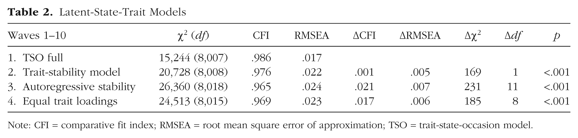
Note: CFI = comparative fit index; RMSEA = root mean square error of approximation; TSO = trait-state-occasion model.

Variance components

Table 3 and Figure 2 depict the different amounts of model variance explained by the trait and state factors. Because the amount of variance explained by state factors (and autoregressions) differs at each wave, the remaining variance per wave explained by the trait factor changes in line with this, although this is summed to form the overall variance explained across the whole model by the stable-trait variance. Variance that was explained by the autoregressive factor ranged between 11.9% (Wave 2) and 6.2% (Wave 10). Considering waves in which the autoregressive factor was present (Wave 2 onward), we found that the time-varying variance ranged from 71.6% (Wave 2) to 36.8% (Wave 10). The time-varying component of depression gradually declined during early adolescence to mid-adolescence (71.6% at 13 years, 62.8% at 14 years, 48.2% at 17 years) and reached 42.1% at age 22, where it remained until age 24, after which, the time-varying variance decreased further to 36.8% at age 26. Based on the CIs, the state variance at Wave 1 (age 11) was significantly higher than at all subsequent waves, explaining 91.0% of the total variance (however, note there is no autoregressive factor at this wave). Waves 2 and 3 (ages 13 and 14) also showed significantly higher state variance compared with the later waves; their CIs did not overlap with those of the following waves. Waves 4 through 6 (ages 17–19) had higher point estimates than later waves (around 50%), and their CIs generally did not overlap with subsequent waves. Waves 7 through 10 (ages 22–26) showed similar estimates (dropped to around 40%), with a slight decrease from Wave 8 (age 23) compared with Wave 10 (age 26).

Table 3.

Proportion of Variance Across Waves

	Wave 1	Wave 2	Wave 3	Wave 4	Wave 5	Wave 6	Wave 7	Wave 8	Wave 9	Wave 10
Age	11	13	14	17	18	19	22	23	24	26
Time-invariant	8.1%	16.4%	26.7%	43.7%	40.4%	40.7%	50.8%	49.6%	50.8%	57.0%
95% CI	[4.0, 13.2]	[11.4, 22.6]	[20.2, 33.8]	[37.8, 50.7]	[34.2, .47.2]	[34.1, 47.8]	[44.5, 57.6]	[43.9, 55.9]	[44.9, 57.2]	[51.7, 62.5]
Time-varying	91.9%	71.6%	62.8%	48.2%	51.0%	50.8%	42.1%	43.2%	42.2%	36.8%
95% CI	[96.0, 86.8]	[75.9, 66.4]	[68.4, 56.7]	[53.3, 42.3]	[56.4, 45.3]	[56.5, 44.7]	[47.6, 36.3]	[48.3, 37.7]	[47.2, 36.7]	[41.4, 32.1]
Autoregressive	—	11.9%	10.5%	8.1%	8.6%	8.5	7.1%	7.2%	7.0%	6.2%
95% CI	—	[12.7, 11.0]	[11.4, 9.5]	[8.9, 7.0]	[9.4, 7.6]	[9.4, 7.5]	[7.9, 6.1]	[8.1, 6.4]	[7.9, 6.1]	[6.9, 5.4]

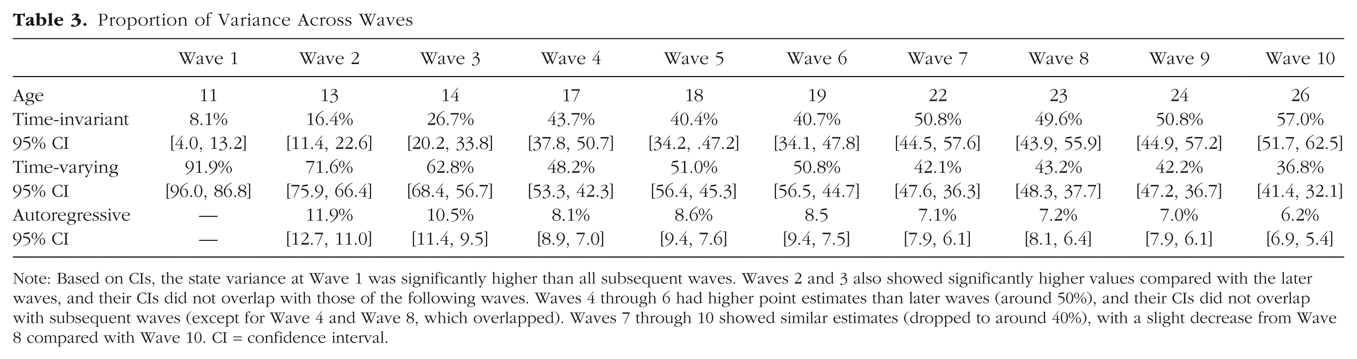
Note: Based on CIs, the state variance at Wave 1 was significantly higher than all subsequent waves. Waves 2 and 3 also showed significantly higher values compared with the later waves, and their CIs did not overlap with those of the following waves. Waves 4 through 6 had higher point estimates than later waves (around 50%), and their CIs did not overlap with subsequent waves (except for Wave 4 and Wave 8, which overlapped). Waves 7 through 10 showed similar estimates (dropped to around 40%), with a slight decrease from Wave 8 compared with Wave 10. CI = confidence interval.

Fig. 2.

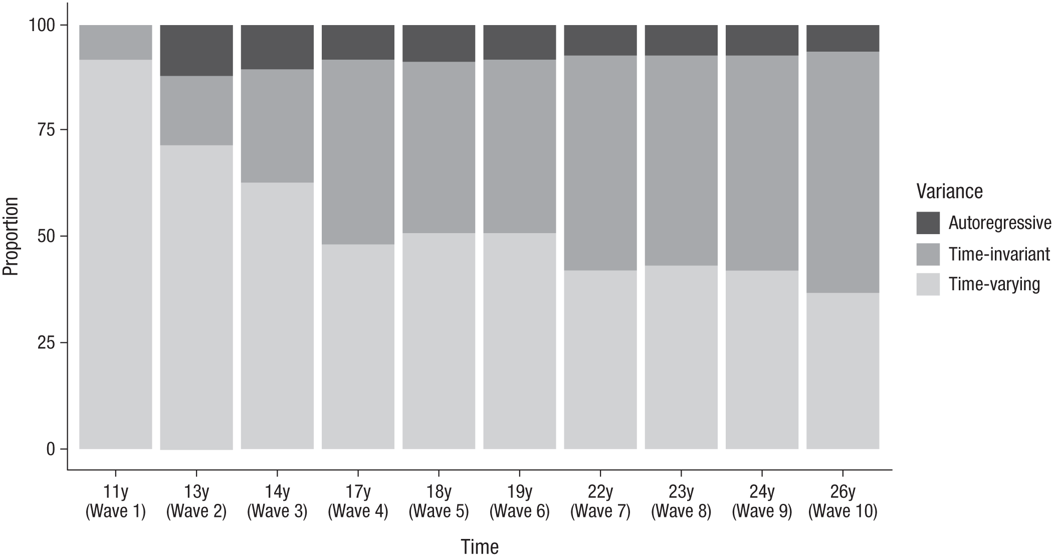
Variance proportions from age 11 to age 26.

Prediction models

Table 4 shows the coefficients of the regression models (for standard errors and test statistic, see Table S3 in the Supplemental Material). We did not detect multicollinearity in our models; all variance inflation factors were below 3. Trait depression was significantly correlated with female sex, more adolescent stressful life events and psychotic symptoms, less school enjoyment in adolescence, more anxiety symptoms, and worse general health in emerging adulthood. Predictor variables explained 49% of the variance in the trait variable. Variables predicting state depression varied with age (for detailed results, see Table 4) and explained between 4% (State 6, 19 years of age) and 24% (State 7, 22% years of age) of the variance. Early predictors at age 11 included higher Strengths and Difficulties Questionnaire scores at age 7 and lower school ability. By age 13, female sex, prior life events, and prior school difficulties were key predictors of state depression. At age 14, factors such as maternal depression, prior life events, and prior school-related variables were important predictors. From age 17 onward, predictors of state depression included sex, maternal depression, life events, and trauma exposure. By age 22, anxiety symptoms became the main predictor (only measured age 22), continuing to influence state depression through age 26. Sensitivity analyses indicated high stability of our results. Estimates remained largely consistent when including predictors of missingness (see Table S4 in the Supplemental Material), bootstrap analyses showed minimal bias and narrow CIs (see Table S5 in the Supplemental Material), and coefficients were broadly similar across the split-half analyses (all overlapping CIs; for details, see Table S6 in the Supplemental Material). In our moderation models, no significant interaction effects were observed, and only some main effects were detected (see Table S7 in the Supplemental Material).

Table 4.

Multivariable Associations^a of the Trait and State Components of Depression From Waves 1 to 10

	Trait	State 1 (11 years)	State 2 (13 years)	State 3 (14 years)	State 4 (17 years)	State 5 (18 years)	State 6 (19 years)	State 7 (22 years)	State 8 (23 years)	State 9 (24 years)	State 10 (26 years)
Adjusted R²	.49	.06	.08	.10	.17	.11	.04	.24	.11	.08	.06
Sex (male)	−0.12***	0.05	−0.16***	−0.32***	−0.44***	−0.32***	−0.13**	0.07	0.06	0.10	−0.06
Temperament, 57 months^b	0.00	0.00	0.00	−0.01	0.00	0.01	0.02	0.01	0.01	0.01	0.00
Maternal depression, 11 years^b	0.05	0.01	0.05	0.09*	0.18***	0.10*	−0.01	0.01	0.09*	0.00	−0.02
Parent–child relationship quality, 14 years	0.00	—	—	—	0.03***	0.02*	−0.02	0.01	0.01	0.02	0.01
Conflict parents, 6.5 years^b	0.01	0.02	0.03	0.03	0.02	−0.02	−0.01	−0.00	−0.03	0.02	0.01
Life events, 12–16 years^c	0.02*	—	0.04***	0.06***	0.07***	0.03**	0.00	−0.01	0.02	−0.02	0.02
Trauma until 11 years^d	0.02	—	0.01	0.02	0.03**	0.03**	−0.01	0.00	0.02	−0.02	0.00
Trauma, 11–17 years^d	0.01	—	0.01	0.01	0.00	0.00	0.02	−0.01	0.00	0.04*	0.01
School ability, 9.7 years	−0.02	−0.06***	−0.07***	−0.06*	−0.03	0.01	0.02	0.00	0.01	−0.01	0.00
School enjoyment, 11.2 years	−0.06	—	−0.16***	−0.09*	−0.09*	−0.09*	0.02	−0.04	−0.02	−0.04	−0.01
School enjoyment, 14.1 years	−0.03*	—	—	—	0.01	0.02	0.03	−0.01	0.05	0.02	0.03
Psychopathology (SDQ total), 6.9 years	0.01	0.02***	0.01	0.01	0.01	0.02***	−0.00	0.01	0.00	−0.01	0.01
Anxiety, 22 years	0.05***	—	—	—	—	—	—	0.07***	0.03***	0.03***	0.02*
Psychotic, 17 years	0.04***	—	—	—	—	—	0.04	−0.02	−0.02	−0.01	0.01
Health problems, 18.7 years	0.07***	—	—	—	—	—	—	−0.01	0.06*	−0.05	−0.05
Health problems, 21 years	0.05	—	—	—	—	—	—	0.05	0.03	0.04	0.04
Health problems, 22 years	0.02	—	—	—	—	—	—	0.01	0.08*	0.07	0.05

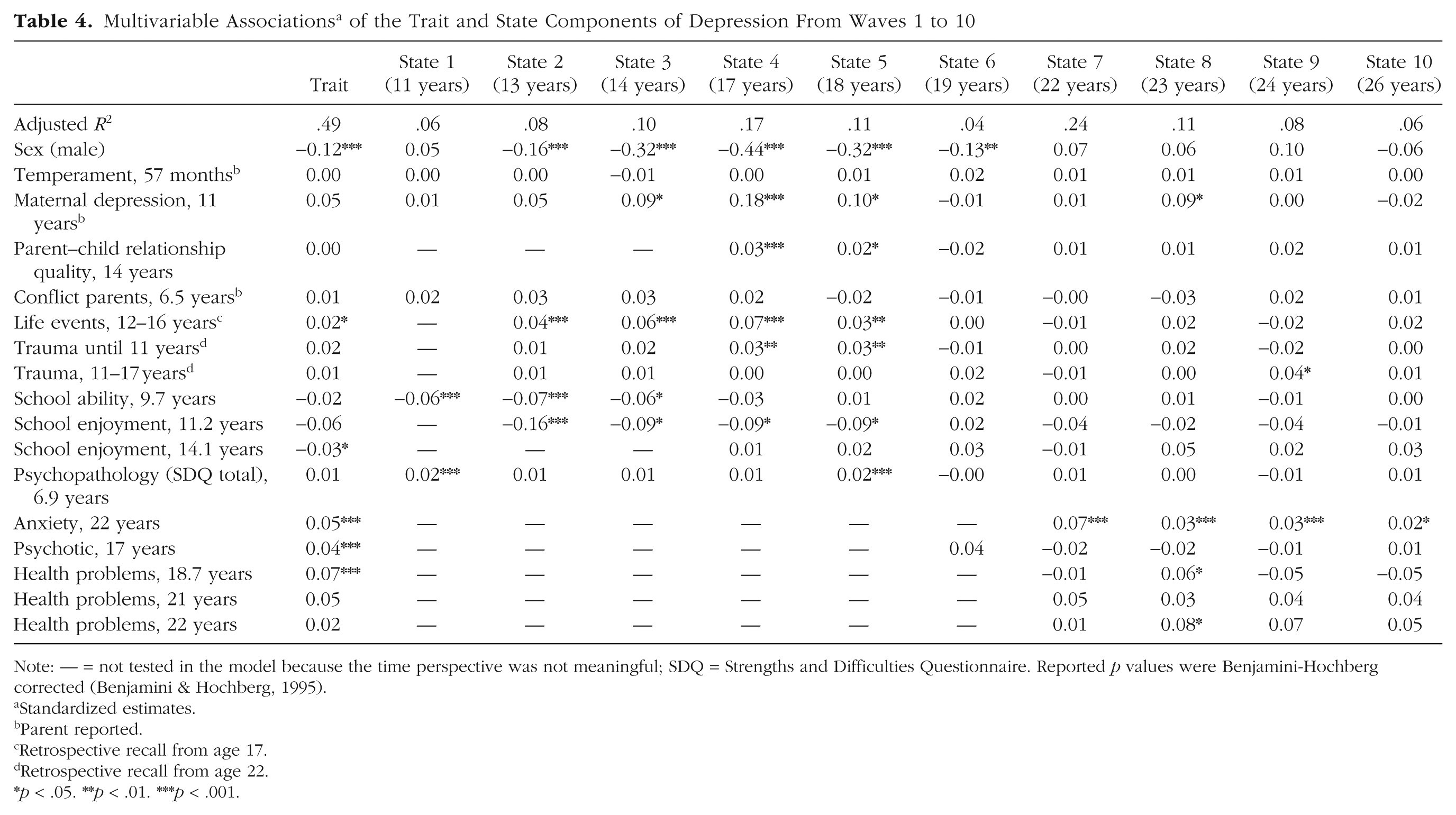
Note: — = not tested in the model because the time perspective was not meaningful; SDQ = Strengths and Difficulties Questionnaire. Reported p values were Benjamini-Hochberg corrected (Benjamini & Hochberg, 1995).

Standardized estimates.

Parent reported.

Retrospective recall from age 17.

Retrospective recall from age 22.

p < .05. **p < .01. ***p < .001.

Discussion

We examined the amount of variance explained by state and trait factors of depression modeled across development from ages 11 to 26 and determined predictors of these factors in a population-based study. The amount of state variance was relatively high from ages 11 to 14, decreased and remained stable at similar levels from ages 17 to 19, and then further decreased and reached a plateau from ages 22 to 26. This magnitude of state variance is higher than percentages reported in former studies of depression, which may be because our study observed change over many more years than prior studies (15 years in our study compared with up to 4 years previously; Cole et al., 2017; Prenoveau, 2016; Wu, 2016). This points to the importance of the time frame because variance that appears to be trait-like across shorter time intervals may become state-like across longer periods of observation (Hamaker, 2023). At age 11, model variance was explained almost completely by the state factor, in line with studies suggesting that this is a time of emergent psychopathology (Solmi et al., 2022). Yet at this age, variance was disaggregated only into state and trait variance without an autoregressive factor, compared with the other waves, which may partly account for the high state variance. At ages 13 and 14, the state factor explained around two-thirds of the model variance, which dropped to explaining around half of the model variance from ages 17 to 19, dropping to around 40% for the remainder of waves (ages 22–26). This increasing stability in depressive symptoms as adolescents age may be due to fewer psychobiological changes, more stable relationships, self-concept, and life circumstances (Dahl et al., 2018; Sawyer et al., 2018). Autoregressive pathways were highest at age 11 (11.9%) and gradually declined to 6.2% at age 26, reflecting characteristics across waves that cannot be explained by the latent factors. These may reflect individual factors, such as family environment, the influence of which typically declines as adolescents age (Arnett, 2000).

The greater role of state factors in early adolescent depression suggests that depression is more modifiable at younger ages (Prenoveau, 2016). Pinpointing the temporal pattern of different predictors of this more labile aspect of depression can critically inform intervention studies. We chose well-known predictors of depression (Thapar et al., 2022) that have not yet been related to the state and trait components of depression.

Female sex was associated with the trait component of depression, in line with previous evidence suggesting that females are more susceptible to depression than males (Salk et al., 2017). State depression was predicted by female sex from ages 12 to 19 but not at age 11. This finding aligns with epidemiological reports that found no differences in the prevalence of depressive symptoms between males and females at age 11, but differences were evident at age 14 (Patalay & Fitzsimons, 2018). However, the present findings increase precision on this observation by indicating that female sex becomes a risk factor for new-onset depression around the age of 12 years. In our study, female sex predicted state depression until the age of 19, after which, sex no longer predicted state depression. This aligns with prior research showing a more pronounced increase in depressive symptoms among females during adolescence (Collishaw, 2015; Shore et al., 2018) and may also point to hormonal effects during puberty that increase vulnerability for depression in females (Hyde et al., 2008; Lewis et al., 2018). After age 19, sex differences seem to be attributable to differences in trait depression. These findings underscore the need for sex-specific interventions during development (Davey & McGorry, 2019), which might stop the low mood that many pubertal girls experience from developing into stable depression.

Maternal depression at age 11 did not predict trait depression but was associated with the emergence of state depression between the ages of 14 and 18 and at age 23. This may reflect an underlying vulnerability for the emergence of depressive symptoms in a sensitive period and an interaction of genes with environment (S. H. Goodman et al., 2011). Maternal depression may impede the mother’s ability to respond to her child’s depressive symptoms effectively and may thus contribute to symptom escalation, potentially also through biological pathways (Olino et al., 2022). Parent–child relationship quality at 14 years of age predicted state depression at the next two waves (ages 17 and 18), a time when adolescents may often feel misunderstood, which may contribute to depressive symptoms (Yap et al., 2014). There was no association with state depression at age 19, which could reflect the fact that many young people would have left home by then, particularly individuals with poorer relationships with their parents, and thus the influence of maternal depression on their child’s symptoms may recede; however, it may also reflect the greater time interval between measurements. However, conflict with parents at age 7 (or child temperament at age 57 months) was not associated with state or trait depression at any measured time point, likely because this was in the distant past and thus may only indirectly contribute to any change in depressive symptoms. These findings underscore the need for identification and treatment of depression in parents and parental psychoeducation to increase awareness of how parental factors relate to the well-being of children. In addition, interventions targeting communication and relationships within the family may be effective in reducing the risk of depression in adolescents (Thapar et al., 2022).

Stressful life events occurring in early adolescence were associated with trait depression and predicted change in state depression both concurrently (ages 13–14) and subsequent to the events (ages 17–18), consistent with studies reporting that life events are related to the onset of adolescent depression (Korten et al., 2012). The present study adds to existing knowledge by pointing to time-varying association at potentially sensitive periods. However, these time-varying associations could become more precise if assessed using more regular measurement of adolescent stressful life events, which in the present study were retrospectively recalled at age 17. Childhood traumatic events (i.e., until the age of 11) were related to state depression from ages 17 to 18. Trauma experienced in adolescence (from ages 11 to 17) predicted change in depressive symptoms at age 24. Although both measures of traumatic events were recalled at age 22, the finding of greater effects of childhood trauma than adolescent trauma on depression at ages 17 to 18 is consistent with prior literature and that overall, life events and trauma have profound effects on young people’s subsequent mental health (Dunn et al., 2018). Childhood trauma was not associated with trait depression, potentially because of the assessment at age 22.

School enjoyment was related to trait and state components of depression until age 18 (when most kids leave school), highlighting the importance of school environments in mental health (Ford et al., 2021). In our analyses, school enjoyment at age 11 was in fact the strongest modifiable child-based predictor of state depression at ages 13 to 18, equivalent in effect size to maternal depression. However, school enjoyment at age 14 was associated only with trait depression but not with state depression at any wave. Consistent with a longitudinal meta-analysis on school enjoyment and internalizing symptoms (Huang, 2015), we found that school ability at age 10 predicted state depression from ages 11 to 14. School variables thus appear to affect trait depression and to exert a time-varying influence on depressive symptoms during these critical developmental phases, highlighting the importance of schools monitoring children’s mental health and creating an enjoyable and safe environment (Ford et al., 2021), which is jeopardized in the UK in recent decades with the increase in academic pressure and a narrower academic curriculum (Armitage et al., 2025).

Maternal-reported psychopathology (i.e., child’s problems) at age 7 was associated with state depression at ages 11 and 18, pointing to some predictive effects of early mental-health problems and the importance of prioritizing early and regular mental-health screenings (Davey & McGorry, 2019; R. Goodman, 2001). Yet assessments took place only at a young age, and parental reports of mental-health symptoms are not perfectly reliable (for a meta-analysis, see De Los Reyes et al., 2015), so they may not have captured more nuanced developments of depression in subsequent waves. Psychotic, anxiety, and general health symptoms were all related to trait depression, in line with proposed transdiagnostic models suggesting a high overlap between these conditions (Cummings et al., 2014; St. Clair et al., 2017). However, evidence for temporal perspectives was also found, consistent with prior work showing that self-rated health predicts long-term prognosis of depression (Ambresin et al., 2014) and that anxiety symptoms often precede depression (Keenan et al., 2009). Specifically, anxiety symptoms were associated with state depression at all points after the first anxiety assessment at age 22 until the age of 26. Of the comorbidities, anxiety was the most consistent predictor of depressive symptoms, in line with a range of former studies underscoring this high comorbidity (Cummings et al., 2014; Kessler et al., 2005; Merikangas et al., 2010). These findings point to the need for a regular and holistic assessment of mental-health symptoms across disorders using multiple informants. However, for health conditions, we found inconsistent patterns across ages, which may be attributable to different health conditions at different waves having different impacts on depression.

No significant interaction effects were observed in our moderation models, suggesting that the examined predictors contributed primarily additively to state depression. This may be attributable to characteristics of our study design and assessments. Specifically, several predictors were measured at different developmental time points, which may have limited the temporal overlap necessary to capture interactive effects between factors. At these distinct time points, our predictors may exert their influence on depressive symptoms through partly independent pathways rather than interacting directly. Nonetheless, investigating potential interactions between risk factors remains an important direction for future research. Understanding how child characteristics, family dynamics, and contextual factors jointly influence the emergence of depressive symptoms could clarify mechanisms underlying developmental vulnerability. Future studies with more closely aligned or repeated assessments of these predictors or designs specifically optimized to detect such interplay are crucial to determine whether certain combinations of risk factors confer particularly high risk for state depression.

Limitations of our study are as follows. Caution is needed in interpreting the small effect sizes observed for predictors of both state and trait depression, which were smaller than effect sizes typically found in regression models predicting depression sum scores (Shore et al., 2018). For example, the correlation between mothers’ depression and children’s internalizing symptoms was r = .23 (S. H. Goodman et al., 2011). The association between trauma severity and depression was r = .20 in children and adolescents (Claxton et al., 2021). More in line with our findings, there were small associations between depression and school absenteeism (r = .11; Finning et al., 2019) and academic achievement and subsequent depression (r = –.15; Huang, 2015). The relatively small effect sizes in our study may be explained by a smaller amount of variance in our multiple-regression models than in models that predict depression as a whole (Shore et al., 2018). This aligns with our prior study that tested predictors of state and trait components of distress during COVID-19, also using a TSO model (Schlechter, Ford, et al., 2023). The practical relevance of these effect sizes remains thus uncertain because there is currently limited existing literature on predictors of partitioned trait and state factors. However, given that there is potentially more understanding of what is being predicted at a given point in time (stable or time-varying component of depression), Cole (2006) argued these partitioned effect sizes are more meaningful. Furthermore, the strength of effect is consistent with studies that disentangled between-persons (i.e., trait factors) and within-persons variance (i.e., state factors; Curran & Bauer, 2011). Although stable differences between persons may be more robust than changes that fluctuate within individuals over time, small changes in depression over time may accumulate and lead to important long-term effects, which can eventually become trait-like. Because the present findings stem from a population-based study, even small effects sizes may be meaningful if they affect many people (Carey et al., 2023; Greenberg & Abenavoli, 2017).

Importantly, despite demonstrating high stability in sensitivity analysis within our sample, our results remain sample dependent. Consequently, replication in independent cohorts is necessary to determine whether the observed patterns reflect true effects or are influenced by specific characteristics of our sample. Such replication would help clarify whether the findings are attributable to differences in the timing of assessments (e.g., developmental factors), retrospective recall period of the measure, or chance. Furthermore, our findings lack comparability with former TSO studies because of the use of different time frames of study during a sensitive period of development (Wu, 2016). Cross-validation is therefore necessary to discern whether our findings would replicate in a similar cohort, considering factors such as age range and number of years studied, frequency of measurement, and type of population. In addition, we lacked more detailed indicators of gender, cultural backgrounds, and socioeconomic status, which should be considered in future research. Specifically, cross-validation in culturally and socioeconomically diverse samples is needed because ALSPAC participants were more likely to have higher education and be White and were less likely to receive free school meals compared with representative cohorts (Boyd et al., 2013). A further limitation is the time frame used in the SMFQ. Because the SMFQ asks participants to report symptoms over the past 2 weeks, it may capture more short-term fluctuations, which could have contributed to higher estimates of state variance (Hamaker, 2023). Furthermore, the internal consistency of the SMFQ increased across later assessment waves. Yet latent-variable modeling accounts for measurement error at each wave, so the observed decrease in state variance is unlikely to be solely due to improved reliability. In addition, our use of variables to predict disentangled trait and state components of depression is unique. These predictors themselves could not be disaggregated into trait and state components because they were assessed inconsistently throughout the study period. For future studies, it could be worthwhile to investigate how, for example, time-invariant and time-varying anxiety symptoms relate to different variance components of depression. In this regard, choosing the appropriate time window to capture these cumulative effects and ensuring time-varying predictors have a similar time frame to outcomes is important and should be informed by developmental theories. Finally, trauma history and life events were assessed retrospectively. We used them to predict variance around the time of their occurrence, so their estimates may be biased by retrospective reports.

Conclusion

The current study contributes to the understanding of the temporal stability of depression across a developmental period spanning early adolescence to emerging adulthood. We found that the state depression was particularly high during early adolescence (ages 11–14), underscoring the critical importance of this developmental stage for the emergence of depression. Through the identification of key predictors of state depression, ranging from family factors to other mental-health conditions, our study offers a valuable foundation for future research, which may ultimately inform studies developing and testing targeted intervention strategies within critical windows of vulnerability.

Supplemental Material

sj-docx-1-cpx-10.1177_21677026261422140 – Supplemental material for Predictors of State and Trait Components of Depression From Early Adolescence Into Emerging Adulthood

Supplemental material, sj-docx-1-cpx-10.1177_21677026261422140 for Predictors of State and Trait Components of Depression From Early Adolescence Into Emerging Adulthood by Pascal Schlechter, Tamsin Ford, Paul O. Wilkinson and Sharon A. S. Neufeld in Clinical Psychological Science

Footnotes

Acknowledgements

We are extremely grateful to all the families who took part in this study, the midwives for their help in recruiting them, and the whole Avon Longitudinal Study of Parents and Children team, which includes interviewers, computer and laboratory technicians, clerical workers, research scientists, volunteers, managers, receptionists, and nurses. The views and opinions expressed therein are those of the authors and do not necessarily reflect those of the National Institute for Health Research, National Health Service, or the Department of Health and Social Care. This publication is the work of the authors, and P. Schlechter, P. O. Wilkinson, T. Ford, and S. A. S. Neufeld serve as guarantors for the contents of this article.

Transparency

Action Editor: Jennifer L. Tackett

Editor: Jennifer L. Tackett

Author Contributions

Pascal Schlechter: Conceptualization; Formal analysis; Investigation; Methodology; Writing – original draft.

Tamsin Ford: Investigation; Methodology; Supervision; Writing – review & editing.

Paul O. Wilkinson: Conceptualization; Methodology; Supervision; Writing – review & editing.

Sharon A. S. Neufeld: Conceptualization; Formal analysis; Investigation; Methodology; Supervision; Writing – original draft.

ORCID iDs

Pascal Schlechter

Sharon A. S. Neufeld

Supplemental Material

Additional supporting information can be found at

References

Ambresin

Chondros

Dowrick

Herrman

Gunn

J. M.

(2014). Self-rated health and long-term prognosis of depression. The Annals of Family Medicine, 12(1), 57–65. https://doi.org/10.1370/afm.1562

Angold

Costello

E. J.

Messer

S. C.

Pickles

(1995). Development of a short questionnaire for use in epidemiological studies of depression in children and adolescents. International Journal of Methods in Psychiatric Research, 5, 237–249.

Armitage

J. M.

Lewis

Page

Tseliou

Anthony

Murphy

Moore

Collishaw

(2025). Change over time in perceived schoolwork pressure and associations with emotional problems among 11–16-year-olds: A repeat cross-sectional study in Wales, UK. JCPP Advances, 5(4), Article e70005. https://doi.org/10.1002/jcv2.70005

Arnett

J. J.

(2000). Emerging adulthood: A theory of development from the late teens through the twenties. American Psychologist, 55(5), 469–480. https://doi.org/10.1037/0003-066X.55.5.469

Asparouhov

Muthén

(2010). Weighted least squares estimation with missing data. Mplus Technical Appendix, 2010(5), 1–10.

Benjamini

Hochberg

(1995). Controlling the false discovery rate: A practical and powerful approach to multiple testing. Journal of the Royal Statistical Society Series B: Methodological, 57(1), 289–300.

Bould

Joinson

Sterne

Araya

(2013). The Emotionality Activity Sociability Temperament Survey: Factor analysis and temporal stability in a longitudinal cohort. Personality and Individual Differences, 54(5), 628–633. https://doi.org/10.1016/j.paid.2012.11.010

Boyd

Golding

Macleod

Lawlor

Fraser

Henderson

Molloy

Ness

Ring

Davey Smith

(2013). Cohort profile: The ‘Children of the 90s’-The index offspring of the Avon Longitudinal Study of Parents and Children. International Journal of Epidemiology, 42(1), 111–127. https://doi.org/10.1093/ije/dys064

Buss

Plomin

(1984). Temperament: Early developing personality traits. Hillsdale, NJ: Lawrence Erlbaum.

10.

Carey

E. G.

Ridler

Ford

T. J.

Stringaris

(2023). Editorial perspective: When is a ‘small effect’ actually large and impactful? Journal of Child Psychology and Psychiatry, 64(11), 1643–1647. https://doi.org/10.1111/jcpp.13817

11.

Chen

Garnier-Villarreal

Kite

B. A.

Jia

(2020). Testing measurement invariance with ordinal missing data: A comparison of estimators and missing data techniques. Multivariate Behavioral Research, 55(1), 87–101. https://doi.org/10.1080/00273171.2019.1608799

12.

Claxton

Vibhakar

Allen

Finn

Gee

Meiser-Stedman

(2021). Risk factors for depression in trauma-exposed children and adolescents: A systematic review and meta-analysis. Journal of Affective Disorders Reports, 5, Article 100150. https://doi.org/10.1016/j.jadr.2021.100150

13.

Cole

D. A.

Martin

N. C.

Steiger

J. H.

(2005). Empirical and conceptual problems with longitudinal trait-state Models: Introducing a trait-state-occasion model. Psychological Methods, 10(1), 3–20. https://doi.org/10.1037/1082-989X.10.1.3

14.

Cole

D. A.

(2006). Coping with longitudinal data in research on developmental psychopathology. International Journal of Behavioral Development, 30(1), 20–25. https://doi.org/10.1177/0165025406059969

15.

Cole

D. A.

Martin

J. M.

Jacquez

F. M.

Tram

J. M.

Zelkowitz

Nick

E. A.

Rights

J. D.

(2017). Time-varying and time-invariant dimensions of depression in children and adolescents: Implications for cross-informant agreement. Journal of Abnormal Psychology, 126, 635–651. https://doi.org/10.1037/abn0000267

16.

Collishaw

(2015). Annual research review: Secular trends in child and adolescent mental health. Journal of Child Psychology and Psychiatry, 56(3), 370–393. https://doi.org/10.1111/jcpp.12372

17.

Cummings

C. M.

Caporino

N. E.

Kendall

P. C.

(2014). Comorbidity of anxiety and depression in children and adolescents: 20 years after. Psychological Bulletin, 140, 816–845. https://doi.org/10.1037/a0034733

18.

Curran

P. J.

Bauer

D. J.

(2011). The disaggregation of within-person and between-person effects in longitudinal models of change. Annual Review of Psychology, 62, 583–619. https://doi.org/10.1146/annurev.psych.093008.100356

19.

Dahl

R. E.

Allen

N. B.

Wilbrecht

Suleiman

A. B.

(2018). Importance of investing in adolescence from a developmental science perspective. Nature, 554, 441–450. https://doi.org/10.1038/nature25770

20.

Davey

C. G.

McGorry

P. D.

(2019). Early intervention for depression in young people: A blind spot in mental health care. The Lancet Psychiatry, 6(3), 267–272. https://doi.org/10.1016/S2215-0366(18)30292-X

21.

De Los Reyes

Augenstein

T. M.

Wang

Thomas

S. A.

Drabick

D. A. G.

Burgers

D. E.

Rabinowitz

. (2015). The validity of the multi-informant approach to assessing child and adolescent mental health. Psychological Bulletin, 141, 858–900. https://doi.org/10.1037/a0038498

22.

Dunn

E. C.

Soare

T. W.

Raffeld

M. R.

Busso

D. S.

Crawford

K. M.

Davis

K. A.

Fisher

V. A.

Slopen

Smith

A. D. A. C.

Tiemeier

Susser

E. S.

(2018). What life course theoretical models best explain the relationship between exposure to childhood adversity and psychopathology symptoms: Recency, accumulation, or sensitive periods? Psychological Medicine, 48(15), 2562–2572. https://doi.org/10.1017/S0033291718000181

23.

Elovainio

Jokela

Rosenström

Pulkki-Råbäck

Hakulinen

Josefsson

Hintsanen

Hintsa

Raitakari

O. T.

Keltikangas-Järvinen

(2015). Temperament and depressive symptoms: What is the direction of the association? Journal of Affective Disorders, 170, 203–212. https://doi.org/10.1016/j.jad.2014.08.040

24.

Finning

Ukoumunne

O. C.

Ford

Danielsson-Waters

Shaw

Romero

Jager

Stentiford

Moore

D. A.

(2019). The association between child and adolescent depression and poor attendance at school: A systematic review and meta-analysis. Journal of Affective Disorders, 245, 928–938. https://doi.org/10.1016/j.jad.2018.11.055

25.

Ford

Esposti

M. D.

Crane

Taylor

Montero-Marín

Blakemore

S.-J.

Bowes

Byford

Dalgleish

Greenberg

M. T.

Nuthall

Phillips

Raja

Ukoumunne

O. C.

Viner

R. M.

Williams

J. M. G.

Allwood

Aukland

Casey

. . . Kuyken

(2021). The role of schools in early adolescents’ mental health: Findings from the MYRIAD study. Journal of the American Academy of Child & Adolescent Psychiatry, 60(12), 1467–1478. https://doi.org/10.1016/j.jaac.2021.02.016

26.

Fraser

Macdonald-Wallis

Tilling

Boyd

Golding

Davey Smith

Henderson

Macleod

Molloy

Ness

(2013). Cohort profile: The Avon Longitudinal Study of Parents and Children: ALSPAC mothers cohort. International Journal of Epidemiology, 42(1), 97–110.

27.

Goodman

(2001). Psychometric properties of the Strengths and Difficulties Questionnaire. Journal of the American Academy of Child & Adolescent Psychiatry, 40(11), 1337–1345. https://doi.org/10.1097/00004583-200111000-00015

28.

Goodman

S. H.

Rouse

M. H.

Connell

A. M.

Broth

M. R.

Hall

C. M.

Heyward

(2011). Maternal depression and child psychopathology: A meta-analytic review. Clinical Child and Family Psychology Review, 14(1), 1–27. https://doi.org/10.1007/s10567-010-0080-1

29.

Greenberg

M. T.

Abenavoli

(2017). Universal interventions: Fully exploring their impacts and potential to produce population-level impacts. Journal of Research on Educational Effectiveness, 10(1), 40–67. https://doi.org/10.1080/19345747.2016.1246632

30.

Hamaker

E. L.

(2023). The within-between dispute in cross-lagged panel research and how to move forward. Psychological Methods. Advance online publication. https://doi.org/10.1037/met0000600

31.

Hammen

(2016). Depression and stressful environments: Identifying gaps in conceptualization and measurement. Anxiety, Stress, & Coping, 29(4), 335–351. https://doi.org/10.1080/10615806.2015.1134788

32.

Harris

P. A.

Taylor

Thielke

Payne

Gonzalez

Conde

J. G.

(2009). Research Electronic Data Capture (REDCap)—A metadata-driven methodology and workflow process for providing translational research informatics support. Journal of Biomedical Informatics, 42(2), 377–381. https://doi.org/10.1016/j.jbi.2008.08.010

33.

Herrman

Patel

Kieling

Berk

Buchweitz

Cuijpers

Furukawa

T. A.

Kessler

R. C.

Kohrt

B. A.

Maj

(2022). Time for united action on depression: A Lancet–World Psychiatric Association Commission. The Lancet, 399(10328), 957–1022. https://doi.org/10.1016/S0140-6736(21)02141-3

34.

Holsen

Kraft

Vittersø

(2000). Stability in depressed mood in adolescence: Results from a 6-year longitudinal panel study. Journal of Youth and Adolescence, 29(1), 61–78. https://doi.org/10.1023/A:1005121121721

35.

Hölzel

Härter

Reese

Kriston

(2011). Risk factors for chronic depression—A systematic review. Journal of Affective Disorders, 129(1), 1–13. https://doi.org/10.1016/j.jad.2010.03.025

36.

Horwood

Salvi

Thomas

Duffy

Gunnell

Hollis

Lewis

Menezes

Thompson

Wolke

Zammit

Harrison

(2008). IQ and non-clinical psychotic symptoms in 12-year-olds: Results from the ALSPAC birth cohort. The British Journal of Psychiatry, 193(3), 185–191. https://doi.org/10.1192/bjp.bp.108.051904

37.

Bentler

P. M.

(1999). Fit indices in covariance structure modeling: Sensitivity to underparameterized model misspecification. Psychological Methods, 3, 424–453. https://doi.org/10.1037/1082-989X.3.4.424

38.

Huang

(2015). Academic achievement and subsequent depression: A meta-analysis of longitudinal studies. Journal of Child and Family Studies, 24, 434–442. https://doi.org/10.1007/s10826-013-9855-6

39.

Hyde

J. S.

Mezulis

A. H.

Abramson

L. Y.

(2008). The ABCs of depression: Integrating affective, biological, and cognitive models to explain the emergence of the gender difference in depression. Psychological Review, 115(2), 291–313. https://doi.org/10.1037/0033-295X.115.2.291

40.

Jenness

J. L.

Peverill

King

K. M.

Hankin

B. L.

McLaughlin

K. A.

(2019). Dynamic associations between stressful life events and adolescent internalizing psychopathology in a multiwave longitudinal study. Journal of Abnormal Psychology, 128(6), 596–609. https://doi.org/10.1037/abn0000450

41.

Joinson

Heron

Araya

Paus

Croudace

Rubin

Marcus

Lewis

(2012). Association between pubertal development and depressive symptoms in girls from a UK cohort. Psychological Medicine, 42(12), 2579–2589. https://doi.org/10.1017/S003329171200061X

42.

Keenan

Feng

Hipwell

Klostermann

(2009). Depression begets depression: Comparing the predictive utility of depression and anxiety symptoms to later depression. Journal of Child Psychology and Psychiatry, 50(9), 1167–1175. https://doi.org/10.1111/j.1469-7610.2009.02080.x

43.

Kessler

R. C.

Berglund

Demler

Jin

Merikangas

K. R.

Walters

E. E.

(2005). Lifetime prevalence and age-of-onset distributions of DSM-IV disorders in the national comorbidity survey replication. Archives of General Psychiatry, 62(6), 593–602. https://doi.org/10.1001/archpsyc.62.6.593

44.

Kessler

R. C.

McLaughlin

K. A.

Green

J. G.

Gruber

M. J.

Sampson

N. A.

Zaslavsky

A. M.

Aguilar-Gaxiola

Alhamzawi

A. O.

Alonso

Angermeyer

Benjet

Bromet

Chatterji

de Girolamo

Demyttenaere

Fayyad

Florescu

Gal

Gureje

. . . Williams

D. R.

(2010). Childhood adversities and adult psychopathology in the WHO World Mental Health Surveys. The British Journal of Psychiatry, 197(5), 378–385. https://doi.org/10.1192/bjp.bp.110.080499

45.

Klein

D. N.

Kotov

Bufferd

S. J.

(2011). Personality and depression: Explanatory models and review of the evidence. Annual Review of Clinical Psychology, 7(1), 269–295. https://doi.org/10.1146/annurev-clinpsy-032210-104540

46.

Köhler

Chrysanthou

Guhn

Sterzer

(2019). Differences between chronic and nonchronic depression: Systematic review and implications for treatment. Depression and Anxiety, 36(1), 18–30. https://doi.org/10.1002/da.22835

47.

Korten

N. C. M.

Comijs

H. C.

Lamers

Penninx

B. W. J. H

. (2012). Early and late onset depression in young and middle aged adults: Differential symptomatology, characteristics and risk factors? Journal of Affective Disorders, 138(3), 259–267. https://doi.org/10.1016/j.jad.2012.01.042

48.

Kwong

A. S.

(2019). Examining the longitudinal nature of depressive symptoms in the Avon Longitudinal Study of Parents and Children (ALSPAC). Wellcome Open Research, 4, Article 126. https://doi.org/10.12688/wellcomeopenres.15395.2

49.

LaGrange

Cole

D. A.

Jacquez

Ciesla

Dallaire

Pineda

Truss

Weitlauf

Tilghman-Osborne

Felton

(2011). Disentangling the prospective relations between maladaptive cognitions and depressive symptoms. Journal of Abnormal Psychology, 120, 511–527. https://doi.org/10.1037/a0024685

50.

LeMoult

Humphreys

K. L.

Tracy

Hoffmeister

J.-A.

Gotlib

I. H.

(2020). Meta-analysis: Exposure to early life stress and risk for depression in childhood and adolescence. Journal of the American Academy of Child & Adolescent Psychiatry, 59(7), 842–855. https://doi.org/10.1016/j.jaac.2019.10.011

51.

Lewis

Ioannidis

van Harmelen

A.-L.

Neufeld

Stochl

Lewis

Jones

P. B.

Goodyer

(2018). The association between pubertal status and depressive symptoms and diagnoses in adolescent females: A population-based cohort study. PLoS One, 13(6), Article e0198804. https://doi.org/10.1371/journal.pone.0198804

52.

Liu

Yang

Feng

Zhao

Lyu

(2020). Changes in the global burden of depression from 1990 to 2017: Findings from the Global Burden of Disease study. Journal of Psychiatric Research, 126, 134–140. https://doi.org/10.1016/j.jpsychires.2019.08.002

53.

Liu

Millsap

R. E.

West

S. G.

Tein

J.-Y.

Tanaka

Grimm

K. J.

(2017). Testing measurement invariance in longitudinal data with ordered-categorical measures. Psychological Methods, 22, 486–506. https://doi.org/10.1037/met0000075

54.

Löwe

Decker

Müller

Brähler

Schellberg

Herzog

Herzberg

P. Y.

(2008). Validation and standardization of the Generalized Anxiety Disorder Screener (GAD-7) in the general population. Medical Care, 46(3), 266–274. https://doi.org/10.1097/MLR.0b013e318160d093

55.

Lin

(2024). Global burden of depression or depressive symptoms in children and adolescents: A systematic review and meta-analysis. Journal of Affective Disorders, 354, 553–562. https://doi.org/10.1016/j.jad.2024.03.074

56.

Mason

W. A.

Chmelka

M. B.

Trudeau

Spoth

R. L.

(2017). Gender moderation of the intergenerational transmission and stability of depressive symptoms from early adolescence to early adulthood. Journal of Youth and Adolescence, 46(1), 248–260. https://doi.org/10.1007/s10964-016-0480-8

57.

Masselink

Van Roekel

Hankin

B. L.

Keijsers

Lodder

G. M. A.

Vanhalst

Verhagen

Young

J. F.

Oldehinkel

A. J.

(2018). The longitudinal association between self-esteem and depressive symptoms in adolescents: Separating between–person effects from within–person effects. European Journal of Personality, 32(6), 653–671. https://doi.org/10.1002/per.2179

58.

McLaughlin

K. A.

Greif Green

Gruber

M. J.

Sampson

N. A.

Zaslavsky

A. M.

Kessler

R. C.

(2012). Childhood adversities and first onset of psychiatric disorders in a national sample of US adolescents. Archives of General Psychiatry, 69(11), 1151–1160. https://doi.org/10.1001/archgenpsychiatry.2011.2277

59.

Merikangas

K. R.

Burstein

Swanson

S. A.

Avenevoli

Cui

Benjet

Georgiades

Swendsen

(2010). Lifetime prevalence of mental disorders in U.S. adolescents: Results from the National Comorbidity Survey Replication–Adolescent supplement (NCS-A). Journal of the American Academy of Child & Adolescent Psychiatry, 49(10), 980–989. https://doi.org/10.1016/j.jaac.2010.05.017

60.

Morken

I. S.

Viddal

K. R.

Ranum

Wichstrøm

(2021). Depression from preschool to adolescence – Five faces of stability. Journal of Child Psychology and Psychiatry, 62(8), 1000–1009. https://doi.org/10.1111/jcpp.13362

61.

Muthén

B. O.

(1998). Mplus technical appendices. Muthén & Muthén.

62.

Northstone

Lewcock

Groom

Boyd

Macleod

Timpson

Wells

(2019). The Avon Longitudinal Study of Parents and Children (ALSPAC): An update on the enrolled sample of index children in 2019. Wellcome Open Research, 4, Article 51. https://doi.org/10.12688/wellcomeopenres.15132.1

63.

Olino

T. M.

Finsaas

M. C.

Dyson

M. W.

Carlson

G. A.

Klein

D. N.

(2022). A multimethod, multiinformant study of early childhood temperament and depression and anxiety symptoms in adolescence. Journal of Psychopathology and Clinical Science, 131(7), 741–753. https://doi.org/10.1037/abn0000769

64.

Patalay

Fitzsimons

(2018). Development and predictors of mental ill-health and wellbeing from childhood to adolescence. Social Psychiatry and Psychiatric Epidemiology, 53(12), 1311–1323. https://doi.org/10.1007/s00127-018-1604-0

65.

Polanczyk

G. V.

Salum

G. A.

Sugaya

L. S.

Caye

Rohde

L. A.

(2015). Annual research review: A meta-analysis of the worldwide prevalence of mental disorders in children and adolescents. Journal of Child Psychology and Psychiatry, 56(3), 345–365. https://doi.org/10.1111/jcpp.12381

66.

Prenoveau

J. M.

(2016). Specifying and interpreting latent state–trait models with autoregression: An illustration. Structural Equation Modeling: A Multidisciplinary Journal, 23(5), 731–749. https://doi.org/10.1080/10705511.2016.1186550

67.

Prenoveau

J. M.

Craske

M. G.

Zinbarg

R. E.

Mineka

Rose

R. D.

Griffith

J. W.

(2011). Are anxiety and depression just as stable as personality during late adolescence? Results from a three-year longitudinal latent variable study. Journal of Abnormal Psychology, 120, 832–843. https://doi.org/10.1037/a0023939

68.

R Core Team. (2021). R: A language and environment for statistical computing. R Foundation for Statistical Computing.

69.

Rohde

Lewinsohn

P. M.

Klein

D. N.

Seeley

J. R.

Gau

J. M.

(2013). Key characteristics of major depressive disorder occurring in childhood, adolescence, emerging adulthood, and adulthood. Clinical Psychological Science, 1(1), 41–53. https://doi.org/10.1177/2167702612457599

70.

Rohde

Lewinsohn

P. M.

Seeley

J. R.

(1991). Are people changed by the experience of having an episode of depression? A further test of the scar hypothesis. Journal of Abnormal Psychology, 99(3), 264–271. https://doi.org/10.1037/0021-843X.99.3.264

71.

Rohde

Lewinsohn

P. M.

Seeley

J. R.

(1994). Are adolescents changed by an episode of major depression? Journal of the American Academy of Child & Adolescent Psychiatry, 33(9), 1289–1298. https://doi.org/10.1097/00004583-199411000-00010

72.

Rosseel

(2012). lavaan: An R package for structural equation modeling. Journal of Statistical Software, 48, 1–36. https://doi.org/10.18637/jss.v048.i02

73.

Salk

R. H.

Hyde

J. S.

Abramson

L. Y.

(2017). Gender differences in depression in representative national samples: Meta-analyses of diagnoses and symptoms. Psychological Bulletin, 143, 783–822. https://doi.org/10.1037/bul0000102

74.

Sawyer

S. M.

Azzopardi

P. S.

Wickremarathne

Patton

G. C.

(2018). The age of adolescence. The Lancet Child & Adolescent Health, 2(3), 223–228. https://doi.org/10.1016/S2352-4642(18)30022-1

75.

Schlechter

Ford

T. J.

McManus

Neufeld

S. A.

(2023). Predictors of time-varying and time-invariant components of psychological distress during COVID-19 in the UK Household Longitudinal Study (understanding society). Psychological Assessment, 35(11), 959–973. https://doi.org/10.1037/pas0001237

76.

Schlechter

Rohde

Seeley

J. R.

Klein

D. N.

Olino

T. M.

(2024). Examining the influence of episode number and age of onset on individual depressive symptoms across episodes of major depression. Journal of Psychiatric Research, 175, 405–410. https://doi.org/10.1016/j.jpsychires.2024.05.039

77.

Schlechter

Wilkinson

P. O.

Ford

T. J.

Neufeld

S. A.

(2023). The Short Mood and Feelings Questionnaire from adolescence to emerging adulthood: Measurement invariance across time and sex. Psychological Assessment, 35(5), 405–418. https://doi.org/10.1037/pas0001222

78.

Schubert

K. O.

Clark

S. R.

Van

L. K.

Collinson

J. L.

Baune

B. T.

(2017). Depressive symptom trajectories in late adolescence and early adulthood: A systematic review. Australian & New Zealand Journal of Psychiatry, 51(5), 477–499. https://doi.org/10.1177/0004867417700274

79.

Shore

Toumbourou

J. W.

Lewis

A. J.

Kremer

(2018). Review: Longitudinal trajectories of child and adolescent depressive symptoms and their predictors – A systematic review and meta-analysis. Child and Adolescent Mental Health, 23(2), 107–120. https://doi.org/10.1111/camh.12220

80.

Solmi

Radua

Olivola

Croce

Soardo

Salazar

Pablo

Il Shin

Kirkbride

J. B.

Jones

Kim

J. H.

Kim

J. Y.

Carvalho

A. F.

Seeman

M. V.

Correll

C. U.

Fusar-Poli

(2022). Age at onset of mental disorders worldwide: Large-scale meta-analysis of 192 epidemiological studies. Molecular Psychiatry, 27(1), Article 1. https://doi.org/10.1038/s41380-021-01161-7

81.

St. Clair

M. C. S.

Neufeld

Jones

P. B.

Fonagy

Bullmore

E. T.

Dolan

R. J.

Moutoussis

Toseeb

Goodyer

I. M

. (2017). Characterising the latent structure and organisation of self-reported thoughts, feelings and behaviours in adolescents and young adults. PLoS One, 12(4), Article e0175381. https://doi.org/10.1371/journal.pone.0175381

82.

Stochl

Khandaker

G. M.

Lewis

Perez

Goodyer

I. M.

Zammit

. . . Jones

P. B.

(2015). Mood, anxiety and psychotic phenomena measure a common psychopathological factor. Psychological Medicine, 45(7), doi:10.1017/S003329171400261X 1483–1493.

83.

Thapar

Eyre

Patel

Brent

(2022). Depression in young people. The Lancet, 400(10352), 617–631. https://doi.org/10.1016/S0140-6736(22)01012-1

84.

Turner

Joinson

Peters

T. J.

Wiles

Lewis

(2014). Validity of the Short Mood and Feelings Questionnaire in late adolescence. Psychological Assessment, 26, 752–762. https://doi.org/10.1037/a0036572

85.

Usami

Murayama

Hamaker

E. L.

(2019). A unified framework of longitudinal models to examine reciprocal relations. Psychological Methods, 24(5), 637–657. https://doi.org/10.1037/met0000210

86.

Vidal Bustamante

C. M.

Rodman

A. M.

Dennison

M. J.

Flournoy

J. C.

Mair

McLaughlin

K. A

. (2020). Within-person fluctuations in stressful life events, sleep, and anxiety and depression symptoms during adolescence: A multiwave prospective study. Journal of Child Psychology and Psychiatry, 61(10), 1116–1125. https://doi.org/10.1111/jcpp.13234

87.

Weavers

Heron

Thapar

A. K.

Stephens

Lennon

Jones

R. B.

Eyre

Anney

R. J.

Collishaw

Thapar

Rice

(2021). The antecedents and outcomes of persistent and remitting adolescent depressive symptom trajectories: A longitudinal, population-based English study. The Lancet Psychiatry, 8(12), 1053–1061. https://doi.org/10.1016/S2215-0366(21)00281-9

88.

Whitaker

K. J.

Vértes

P. E.

Romero-Garcia

Váša

Moutoussis

Prabhu

Weiskopf

Callaghan

M. F.

Wagstyl

Rittman

Tait

Ooi

Suckling

Inkster

Fonagy

Dolan

R. J.

Jones

P. B.

Goodyer

I. M.

, the NSPN Consortium, & Bullmore

E. T

. (2016). Adolescence is associated with genomically patterned consolidation of the hubs of the human brain connectome. Proceedings of the National Academy of Sciences, 113(32), 9105–9110. https://doi.org/10.1073/pnas.1601745113

89.

Wittenborn

A. K.

Rahmandad

Rick

Hosseinichimeh

(2016). Depression as a systemic syndrome: Mapping the feedback loops of major depressive disorder. Psychological Medicine, 46(3), 551–562. https://doi.org/10.1017/S0033291715002044

90.

(2016). Longitudinal Stability of the Beck Depression Inventory II: A latent trait-state-occasion model. Journal of Psychoeducational Assessment, 34(1), 39–53. https://doi.org/10.1177/0734282915582101

91.

Yap

M. B. H.

Pilkington

P. D.

Ryan

S. M.

Jorm

A. F.

(2014). Parental factors associated with depression and anxiety in young people: A systematic review and meta-analysis. Journal of Affective Disorders, 156, 8–23. https://doi.org/10.1016/j.jad.2013.11.007

Supplementary Material

Please find the following supplemental material available below.

For Open Access articles published under a Creative Commons License, all supplemental material carries the same license as the article it is associated with.

For non-Open Access articles published, all supplemental material carries a non-exclusive license, and permission requests for re-use of supplemental material or any part of supplemental material shall be sent directly to the copyright owner as specified in the copyright notice associated with the article.

0.00 MB

0.15 MB