Sage Journals: Discover world-class research

Abstract

There is a significant degree of heterogeneity in scales that purport to measure depression and generalized anxiety in adolescent samples, which makes it difficult to directly compare scores across studies. The aim of the current study is to develop a common metric that facilitates the comparison of scores from different but related scales of depression and generalized anxiety using a large adolescent sample. A nonequivalent-anchor-test design in conjunction with simultaneous calibration was used to equate and develop a common metric for six different scales. The common metric provided scores with acceptable levels of precision across the −1 to 3 range on θ, which represents the more severe and often clinical end of the spectrum. Thus, in the current study, we identified a coherent common metric that is closely aligned with the “distress” subfactor of the Hierarchical Taxonomy of Psychopathology model. Additional validation testing in independent samples is now required.

Keywords

common metric item-response theory distress dimensional

In psychiatric-epidemiological research, there are no standardized biological or laboratory tests that can objectively detect the severity of disorders, identify risk and protective factors associated with disorders, and demonstrate whether population trends have changed across time or cohorts. Instead, observational, cross-sectional, and cohort studies depend on the use of item-based severity or diagnostic scales that are predominantly self-report and generate total scores to represent a construct of interest. Thus, there has been a significant proliferation of scales to measure mental-health constructs that can differ in terms of content, context, and psychometric rigor (Fried, 2017). Indeed, it is rare that different studies use a common set of scales despite purportedly measuring the same or similar constructs. This heterogeneity has made it difficult to standardize mental-health assessment and prevented the comparability of data across studies (Gatz et al., 2015). For example, any differences that emerge between studies may reflect a mix of true differences in the underlying construct and unrelated differences in how the samples respond to the different measures. This may potentially bias results and obfuscate findings from studies that seek to identify long-term trends in mental health to better inform policy and treatment-service planning, complicate studies that draw comparisons across different forms of treatment, and limit studies that seek to increase sample sizes to detect small associations or interactions between mental disorders and other clinically relevant factors (i.e., those examined using individual participant meta-analysis; e.g., Buckman, Saunders, Cohen, et al., 2021; Buckman, Saunders, Stott, et al., 2021; Karyotaki et al., 2021). Indeed, inconsistent measurement limits the potential knowledge gains that could be made from using large and powerful data sets to answer key questions about the nature of and risk for psychopathology (Curran et al., 2018).

The prospect of making significant gains from analyzing large-scale combined data sets has led to calls for international standards that identify a common set of self-report measures for mental health that can be used in studies on adolescent and adult populations moving forward (Farber et al., 2020; Wolpert, 2020). Although this approach is strong in principle, the practical application of a single set of common measures used across different studies may face several barriers that necessitate the use of different measures across studies (Patalay & Fried, 2021). For example, some studies may attempt to reduce respondent burden by giving preference to brief measures, whereas other studies might be more interested in obtaining scores from longer scales with greater precision to detect minor changes in outcomes. Moreover, scale selection depends on how the assessment information will be used; different measures are more ideal for tasks associated with screening compared with diagnosis or assessing individual differences over time. Mental disorders also manifest in numerous forms; some studies may wish to focus on a smaller subset of symptoms while other studies may prefer to focus on broad disorder severity, and different measures will be needed to reflect these different aims. For longitudinal studies, multiple scales measuring the same disorder are required with slight alterations depending on the population under investigation or alterations required to the time frame referred to by each item (e.g., different scales are needed to suit adolescent vs. adult participants). In short, researchers and clinicians often face competing interests. Different measures that purportedly measure the same construct are required across studies or across longitudinal-measurement points for practical reasons, yet to generate accurate comparisons over time or across studies, there is a need to establish a truly comparable score.

To address some of these limitations, researchers have advocated for an alternative approach based on methods that statistically recalibrate and equate different scales, reducing biases associated with differences in scale content and severity, by determining a “common metric” (Kolen & Brennan, 2014). The common-metric approach to standardized measurement has been exemplified in the adult population by the Patient Reported Outcomes Measurement and Information System (PROMIS) to equate existing self- and proxy-reported scales for physical and emotional health (Choi et al., 2014; Cook et al., 2015; Schalet et al., 2014; Schalet, Revicki, et al., 2015; Schalet, Rothrock, et al., 2015). In adolescent/pediatric samples, there have been previous attempts to estimate common metrics that measure depression to facilitate harmonization (Kaat et al., 2020; Olino et al., 2013). Indeed, Kaat and colleagues (2020) found high agreement between PROMIS-pediatric depression scores and those derived from three equated depression scales (Patient Health Questionnaire 9 Adolescent adaptation (PHQ-A); Center for Epidemiological Studies - Depression Child version (CES-DC); Short Mood and Feelings Questionnaire (SMFQ)). According to Bland-Altman plots, the agreement between scores was best for individuals with a higher degree of severity associated with their depressive symptoms.

The method employed by PROMIS involves reestimating scores on existing measures by finding the equivalent scores on the PROMIS item banks for a given construct using a “calibration” sample of participants who complete the PROMIS item bank and additional measures to be equated. However, other studies have developed common metrics using slightly different methods to equate 11 scales that measure depression in the adult general population (Wahl et al., 2014), seven scales that measure psychological distress in an adult community sample (Batterham et al., 2018), and 11 scales that measure social anxiety in an adult community sample (Sunderland et al., 2018) onto a new shared common metric. These studies demonstrated that existing scales can be used to derive scores on an associated common metric with acceptable precision/accuracy and possess a high level of agreement, particularly compared with previously validated cut points on the equated scales that index clinical significance (Wahl et al., 2014). Moreover, Olino and colleagues (2013) found a high degree of convergence (intraclass correlation coefficients [ICCs] ≥ .85) across the two equating approaches (i.e., linking scales to the PROMIS metric compared with equating all items to a single-item pool). Thus, different studies or longitudinal cohorts that use different yet equated scales can use the scoring algorithms to convert scores to the common metric for more accurate comparisons and data harmonization (Gibbons et al., 2014).

In addition to robust methods to equate mental-health scales, a standardized and preferably empirically grounded framework in which to guide and inform the development of common metrics is needed. Previously, mental-health assessments have been established on the basis of the categorical/medical model promoted by the Diagnostic and Statistical Manual (DSM) and the International Classification of Diseases. Indeed, many common metrics discussed above primarily reflect these categorical constructs (e.g., depression, generalized anxiety, social anxiety). However, epidemiological evidence has consistently identified high rates of comorbidity that call into question the categorical-medical model (Andrews et al., 2008, 2009; Krueger, 1999; Slade & Watson, 2006). The presentation of homogeneous symptom clusters across putatively distinct diagnostic constructs, particularly in children and adolescents, indicate that broad or general dimensional traits might better reflect the emergence of psychopathology rather than highly specific diagnostic categories (McElroy et al., 2018). Measurements and metrics that seek to capture psychopathology accurately and validly should aim to strongly reflect how they emerge in nature.

The Hierarchical Taxonomy of Psychopathology (HiTOP) is an empirically driven framework that offers substantial promise as a framework for organizing a set of dimensional constructs that represent broad and specific facets of psychopathology that are linked hierarchically (as observed by higher-order statistical models; Conway et al., 2019; Hyland et al., 2021; Kotov et al., 2017; Ringwald et al., 2021). The HiTOP framework uses dimensional, transdiagnostic latent constructs that attempt to overcome limitations with categorical diagnoses and better capture and reflect comorbidity. One construct that has seen extensive empirical evidence is a midtiered construct in the HiTOP framework, commonly referred to as the “distress” subfactor, that accounts for the extensive co-occurrence between symptoms of depression and chronic worry/generalized anxiety and can be differentiated from other anxiety symptoms that represent the “fear” subfactor (e.g., panic, specific phobias, social anxiety; Forbes et al., 2021). Both distress and fear subfactors have been shown to represent a broader spectrum of “internalizing” that captures the shared variance across all mood and anxiety disorders. Recent evidence has indicated that rates of broad distress and internalizing may emerge in early childhood and become increasingly more specific in later adolescence, manifesting into clinical levels of depression and anxiety in early adulthood (Cervin et al., 2021; McElroy et al., 2018). Thus, it might be possible to use the HiTOP framework to equate measures that purportedly target various signs, symptoms, and features that make up the broader distress subfactor in adolescent samples.

On the basis of this theoretical and empirical background, in the current study, we sought to develop a common metric for broad distress in adolescent samples that can be used to equate multiple measures that target symptoms of depression and chronic worry/generalized anxiety that commonly co-occur. Prior studies have focused on developing either common metrics for more specific constructs, such as depression or social anxiety (Kaat et al., 2020; Olino et al., 2013; Sunderland et al., 2018; Wahl et al., 2014), or broader constructs that target psychological distress/internalizing but have done so in adult populations (Batterham et al., 2018). To our knowledge, no study has examined the possibility of a common metric focusing on comorbid internalizing symptoms (in particular, symptoms indexing the distress subfactor) in an adolescent population. Given adolescence is a time when internalizing symptoms often develop and manifest, it could be argued that a more nonspecific common metric would be suitable for detecting earlier onset cases rather than any disorder-specific metric (McElroy et al., 2018). The aim of the common metric is to provide a single interpretation when combining existing data sets that contain at least one of the equated measures or use the equated scales for research in the future. In the current study, we used data from two large-scale, school-based cohorts to equate six measures designed to measure distress on a common interpretable metric.

Transparency and Openness

The analysis plan for the current study was not preregistered. Code and output files associated with the analysis are available at https://github.com/mmsunderland/disstresscommonmetric. Additional example code required to generate item-response-theory (IRT)-based scoring is provided in the Supplemental Material available online. In the current study, we used secondary data analysis of previously collected samples; the sample-size determination and data exclusions are reported elsewhere (Teesson et al., 2017, 2020). We report all manipulations and measures used in the current study below. The current study received ethical approval from the University of Sydney Human Research Ethics Committee (No. 2020/443).

Method

Sample

Data for the current study were from the baseline collection of two longitudinal, school-based, randomized controlled trials for mental health and substance use. The first study, known as the Climate and Preventure (CAP) study, recruited 26 Australian secondary schools (17 independent and nine government) between September 2011 and February 2012 (Teesson et al., 2017). A total of 2,190 students who received parental consent and consented themselves were eligible to participate. The second sample, known as the Climate Schools Combined (CSC) study, recruited 71 Australian secondary schools from New South Wales, Queensland, and Western Australia between September 2013 and February 2014 (Teesson et al., 2020). A total of 6,386 students who received parental consent and consented themselves were eligible to participate and provided data during at least one collection point. Data from both samples were combined into a harmonized data set (e.g., common items were matched in terms of labeling and response options) that totaled 8,576 students. However, there were some students who had missing data on all variables of interest and were therefore removed from the analysis, resulting in a final analyzed sample size of 8,238 (96%). All data for the current study were deidentified. A random split cross-validation sampling strategy was used to calibrate the common metric and crosswalks in 80% of the data, followed by validating the crosswalks in an independent 20% holdout sample.

The baseline characteristics for the CAP and CSC studies have been presented in previous studies (Teesson et al., 2017, 2020). In brief, the CAP study comprised adolescents with a mean age of 13.4 years (range = 11.9–15.2), 86% of participants were born in Australia, approximately 58% were male, and 82% reported their usual grades on subjects at school were above 70 (out of 100). The CSC study comprised adolescents with a mean age of 13.6 years (range = 11.6–15.5), 82% of participants were born in Australia, approximately 45% were male, and 76% reported their usual grades on subjects at school were above 70 (out of 100). Both studies did not collect information on the racial/ethnic identification of the participating students. The sample broadly reflects Australian school-attending adolescents, albeit the studies had an overrepresentation of adolescents from higher socioeconomic status given recruitment of independent schools. In terms of clinical characteristics, approximately 9.2% scored 13 or above on the Kessler 6, indicating high psychological distress and potential serious mental illness. In contrast, prevalence of psychological distress in a general Australian population sample of adolescents, measured using the Kessler 10, was estimated at 13.3% for high psychological distress and 6.6% for very high psychological distress (Lawrence et al., 2015).

Given that both samples were not administered all scales to be equated, the average number of items with nonmissing responses across the two samples was 29 (SD = 10, range = 5–35). The most common items completed by the sample were from the Kessler 6 Psychological Distress Scale (K6) and Strengths and Difficulties Questionnaire– emotionality (SDQ), which formed the anchor set, followed by the Patient Health Questionnaire-8 (PHQ-8), Generalized Anxiety Disorder seven-item scale (GAD-7), and Child Health Utility instrument (CHU-9D; for details, see Table S1 in the Supplemental Material). The scale with the least number of participants providing data for each item was the Brief Symptom Inventory-depression (BSI-D) subscale (n = 1,538).

Measures

Items that form the common metric were extracted from established mental-health scales that have been widely used and validated. A descriptive summary of all the items and the specific sample they were obtained from are provided in Table S1 in the Supplemental Material.

CHU-9D

The CHU-9D was developed by health economists as a utility function to measure preference-based health-related quality of life among children 7 to 11 years old and has demonstrated validity in adolescents up to the age of 17 (Ratcliffe et al., 2016). The CHU-9D comprises nine questions with five response categories targeting current functioning across domains of worry, sadness, pain, tiredness, annoyance, school, sleep, daily routine, and activities. Previous studies have identified the CHU-9D as a useful proxy measure for mental-health outcomes in routine clinical practice with moderate associations and good discriminate power to detect nonclinical and clinical ranges as determined by the SDQ (Furber & Segal, 2015). Moreover, the CHU-9D has good representation of items that traditionally target internalizing symptoms such as sadness, worry, and irritability.

GAD-7

The GAD-7 was developed as a brief self-report screening tool for generalized anxiety and other anxiety disorders to be administered in public-health and primary-care settings (Spitzer et al., 2006). The scale comprises seven items with a 4-point response scale that targets the frequency of symptoms experienced in the past 2 weeks. The items directly map onto the diagnostic criteria for generalized anxiety disorder of the fifth edition of the DSM (DSM-5), and the scale has been shown to have good predictive properties and validity. More recently, the GAD-7 demonstrated strong associations with a diagnosis of GAD, panic disorder, and social anxiety and other widely used anxiety scales in adolescent populations (Mossman et al., 2017).

PHQ-8

The PHQ-8 is an eight-item measure developed as a valid diagnostic and severity scale for depression symptoms experienced in the past 2 weeks. It has been shown to be a useful depression measure in population-based studies (Kroenke et al., 2009). The PHQ-8 consists of eight items that are included in the PHQ-9; the item targeting suicidal ideation/thoughts of death has been removed. The remaining items each target the frequency of DSM-5 symptoms of depression on a 4-point scale. The PHQ-8 has been shown to be just as useful and valid as the PHQ-9 as a screening tool for depression and more suitable for use in adolescent and school-based samples given the removal of potentially sensitive content (Shin et al., 2019; Wu et al., 2020).

BSI-D

The BSI is a 53-item self-report scale developed to measure nine dimensions (somatization, obsession-compulsion, interpersonal sensitivity, depression, anxiety, hostility, phobic anxiety, paranoid ideation, and psychoticism; Derogatis & Melisaratos, 1983). The current study included the depression subscale, which has previously demonstrated strong validity with a clinical diagnosis of depression, psychological distress, quality of life, and the full mental-health-symptom checklist (Symptom Checklist-90). The depression subscale comprises six items on a 5-point scale that target the current frequency of depressive symptoms.

K6

The K6 was developed as a short form of the Kessler 10 Psychological Distress Scale to rapidly assess psychological distress associated with depression and anxiety in the general-population and primary-care settings (Kessler et al., 2002). The K6 comprises six items measured on a 5-point response scale and has previously demonstrated high levels of internal consistency and fair-to-good predictive ability associated with abnormal scores on the SDQ in adolescents (Mewton et al., 2016).

SDQ

The SDQ is a 25-item scale designed to measure psychological adjustment in children and adolescents. It has been widely used and applied to measure five domains of mental health and distress, including emotional symptoms, conduct problems, hyperactivity-inattention, peer problems, and prosocial behavior. The SDQ has demonstrated excellent convergent validity with other instruments such as the Child Behavior Checklist and the Youth self-report as well as DSM-IV diagnoses (Goodman, 2001). In the current study, we used a self-report version of the SDQ suitable for participants ages 11 to 16, and only the five items from the emotional-symptom subscale were extracted to index internalizing psychopathology.

Statistical analysis

The common metric was developed under the assumption of a nonequivalent-anchor-test design (Dorans, 2007) using IRT. This design allows items from the identified scales across the two samples to be equated using a smaller set of common anchor items that are shared by both samples. In the current study, the two samples were primarily equated using responses obtained from the items on the K6 and the SDQ emotional subscale. The scale-equating algorithms require some degree of commensurability between total scores, suggesting that each of the scales measure a single construct. To evaluate this, we first estimated McDonald’s omega and Cronbach’s alpha coefficients for each scale separately (Dunn et al., 2014). Each scale was also assessed using confirmatory factor analysis (CFA) to evaluate unidimensionality. The CFAs were conducted with the items entered as categorical indicators with a polychoric correlation matrix and a weighted least squares estimator in Mplus version 8.8 (Muthen & Muthen, 2017). Good model fit was determined using a combination of fit statistics, including the confirmatory fit index (CFI; > .95), the Tucker-Lewis fit index (TLI; .95), the root mean square error of approximation (RMSEA; < .08), and the standardized root mean square residual (SRMR; < .08; Hu & Bentler, 1998; Maydeu-Olivares & Joe, 2014).

Items from each scale across both samples were then pooled into a single, large-item pool and simultaneously calibrated using all available information; missing items were treated as missing by design and handled via maximum likelihood estimation. The simultaneous (or concurrent) calibration approach was chosen compared with linking separate calibrations given prior research that suggested better performance of simultaneous calibration (Kim & Cohen, 2016). The graded-response model, as implemented in the mirt package for R, was used to calibrate the items and generate item parameters that were used to convert sum scores to the common metric (Samejima, 1997). Substantively, the graded-response model is used to estimate the ability (or severity) level of each respondent from both samples and identify the location on the severity spectrum and the discrimination associated with each item. The use of simultaneous calibration places items from multiple test forms on the same common metric (estimated with M = 0 and SD = 1), and item parameters generated from the model can be used to generate scores on the common metric from multiple subsets of items (i.e., different test forms). The graded-response model requires additional assumptions to be met of the total-item pool (i.e., essential unidimensionality, local independence, and an absence of differential item functioning for the common items). Testing of the essential unidimensionality assumption was again conducted using CFA of the total-item pool and inspection of standardized factor loadings. The potential impact of unmeasured multidimensionality on a single general factor and the possibility of estimating multidimensional IRT equating were assessed using exploratory-bifactor analysis. The exploratory-bifactor model was estimated using a robust maximum likelihood estimate and an orthogonal bi-geomin rotation provided in Mplus. Additional indices to examine the importance of the single general factor and whether the assumption of essential unidimensional could be made, including the explained common variance, h-index, OmegaH coefficient, and the average relative parameter bias, were estimated from the rotated loadings of the bifactor exploratory-factor-analysis model (Rodriguez et al., 2016).

Local independence was examined by estimating the residual correlation matrix across pairs of items after fitting the single latent dimension. Given that residual correlations require data from complete cases, two subsamples were generated that contained complete case data from the largest number of items across both samples. The first subsample contained the CHU-9D, GAD-7, PHQ-8, K6, and SDQ, and the second subsample contained the BSI-D, K6, and SDQ. Items with pairwise residual correlations that were deemed as high (i.e., >0.3) were flagged as locally dependent as applied in previous IRT-equating studies (Wahl et al., 2014). Finally, differential item functioning of the common items (K6 and SDQ) across sex, sample groups (CAP vs. CSC), and age (above or below 13 years) were examined using the hybrid ordinal logistic regression/IRT method (LORDIF; Choi et al., 2011). This method compares the fit of a series of nested regression models to determine whether the item parameters display greater than trivial levels of differential item functioning. For the current study, the difference between pseudo-R² values for the nested models were used as effect-size measures such that values of 0.02 or higher indexed nontrivial differential item functioning (i.e., greater than a small effect size; Kim et al., 2007).

Items that met all the assumptions were included in the final item calibration. The standard-error curve outlining the degree of precision as a function of the common metric for the total-item pool was generated using the final calibration. In addition, the standard-error curves associated with the individual scales as a function of the common metric were also generated. Crosswalk tables that convert sum scores from each scale to the corresponding value on the common metric were generated using the expected a priori to sum score method proposed by Thissen and colleagues (1995) as well as example syntax to score the common metric using available data in R package mirt (see Appendices A and C in the Supplemental Material). Values on the common metric can be interpreted in two ways. The first involves setting the mean value to 0 and standard deviation to 1 (often labeled “theta scores”), and the second involves setting a mean value of 50 and standard deviation of 10 (often labeled “t scores”). To aid the interpretation of the common metric, previously derived clinical cut points associated with the PHQ-8, GAD-7, K6, and the SDQ were mapped onto the common metric to determine the range of clinical significance. Finally, item-characteristic curves for each item on the common metric were generated as a mechanism to map the highest probabilities of responding to each category of each item from the different scales on the common-metric score (Rothrock et al., 2020).

The crosswalks were then validated in the holdout 20% sample by estimating the theta scores from items administered in the validation sample but using item parameters estimated in the calibration sample. Theta scores were estimated several times using all available items from the full calibration and items from each of the individual scales (e.g., theta scores estimated using only PHQ items, etc.). The estimated theta scores using items from each scale were then compared with the theta scores generated from all available items using the ICC and Bland-Altman plots. A high degree of agreement demonstrates that the scores from the common metric could be reliably estimated using items from just one of the scales that was equated in the current study.

Results

Item-equating assumptions

Scale-level alpha and omega values and CFA fit statistics for the unidimensional model in the calibration sample are provided in Table S2 in the Supplemental Material. Most fit statistics provided evidence for excellent model fit of the unidimensional model for each of the scales according to published cut points. The standardized factor loadings for the single calibration of the total-item pool are provided in Table 1; all factor loadings were greater than 0.4. The strongest factor loadings were associated with items indexing feelings of worthlessness, hopelessness, sadness, loneliness, depression, and uncontrollable worry. The factor loadings for the bifactor model and additional fit indices are provided in Table S3 in the Supplemental Material and provide evidence for a strong general factor accounting for 82% of the common variance and a well-defined latent variable (H = 0.98). The average relative parameter bias indicating the absolute difference between the loadings based on a unidimensional solution and bifactor solution was 0.05 and suggests that the bias due to treating the items as unidimensional is minimal and is not of serious concern (Rodriguez et al., 2016). Inspection of the residual correlation matrices of the two subsamples provided no evidence of substantial local dependence between pairs of items; all pairwise residual correlations less than 0.3 (the average residual correlation for Subsample 1 was 0.01, and Subsample 2 was −0.03). Finally, the results of the LORDIF analysis across sample group (CAP vs. CSC), sex, and age for the K6 and the SDQ items provided no evidence of nontrivial differential item functioning given that differences in pseudo-R² values were less than .02 (see Tables S4 and S5 in the Supplemental Material). Given these findings, the final item pool comprised all 41 items originally included in the analysis.

Table 1.

Item-Level Properties and Item-Bank Parameters

			CFA loading (N = 6,595)	IRT parameters (N = 6,595)
Item name	Brief description	n	CFA loading (N = 6,595)	A1	B1	B2	B3	B4
chu1	Worried	4,798	0.74	1.85	0.60	1.61	2.28	2.93
chu2	Sad	4,800	0.79	2.16	0.86	1.58	2.06	2.71
chu3	Pain	4,799	0.61	1.30	0.75	1.85	2.73	3.58
chu4	Tired	4,799	0.62	1.34	−1.14	0.36	1.17	2.11
chu5	Annoyed	4,798	0.68	1.59	0.56	1.59	2.21	2.82
chu6	Work	4,797	0.61	1.31	0.30	1.70	2.80	3.79
chu7	Sleep	4,794	0.65	1.45	0.18	1.24	2.09	3.00
chu8	Daily routine	4,796	0.70	1.68	1.13	2.15	2.87	3.63
chu9	Able to join in activities	4,797	0.67	1.54	0.89	1.84	2.41	3.37
gad71	Feel nervous, anxious on edge	4,823	0.81	2.38	0.38	1.80	2.52	NA
gad72	Unable to stop or control worrying	4,823	0.87	2.98	0.67	1.61	2.23	NA
gad73	Worrying too much about different things	4,824	0.84	2.62	0.24	1.41	2.08	NA
gad74	Trouble relaxing	4,822	0.83	2.50	0.46	1.54	2.15	NA
gad75	So restless hard to sit still	4,817	0.74	1.88	0.85	1.91	2.60	NA
gad76	Easily annoyed or irritable	4,814	0.77	2.08	−0.02	1.26	1.97	NA
gad77	Afraid something awful might happen	4,819	0.81	2.35	0.49	1.44	1.99	NA
h1suic	Thoughts of ending your life	1,247	0.79	2.22	0.88	1.75	2.14	2.71
h2lonely	Feeling lonely	1,247	0.86	2.87	0.13	1.18	1.73	2.27
h3sad	Feeling sad	1,247	0.86	2.85	−0.25	0.96	1.62	2.12
h4anhedonia	Feeling little interest or pleasure	1,247	0.78	2.14	0.21	1.26	1.98	2.55
h5hopeless	Feeling hopeless	1,247	0.89	3.40	0.53	1.34	1.84	2.19
h6worthless	Feeling worthless	1,247	0.95	4.92	0.61	1.25	1.76	2.09
k61	Nervous	6,587	0.68	1.57	−1.38	0.60	1.97	3.02
k62	Hopeless	6,583	0.81	2.31	0.02	1.01	1.80	2.51
k63	Restless or fidgety	6,575	0.60	1.29	−0.93	0.41	1.70	2.88
k64	So depressed	6,579	0.81	2.38	0.57	1.36	2.00	2.64
k65	Everything was an effort	6,576	0.61	1.30	−0.61	0.67	1.64	2.68
k66	Worthless	6,577	0.83	2.55	0.43	1.17	1.71	2.29
phq1	Feeling down, depressed, irritable, or hopeless	4,856	0.87	3.03	0.52	1.63	2.15	NA
phq2	Little interest or pleasure in doing things	4,853	0.67	1.54	0.35	1.80	2.79	NA
phq3	Trouble falling asleep	4,851	0.72	1.77	−0.13	1.04	1.74	NA
phq4	Poor appetite, weight loss, overeating	4,854	0.73	1.81	0.84	1.74	2.43	NA
phq5	Feeling tired, or little energy	4,854	0.72	1.78	−0.42	1.13	1.92	NA
phq6	Feeling bad about yourself	4,852	0.85	2.75	0.53	1.42	1.98	NA
phq7	Trouble concentrating	4,853	0.76	1.97	0.37	1.58	2.38	NA
phq8	Moving or speaking slowly	4,852	0.76	2.00	1.05	2.01	2.69	NA
sd13	Often unhappy, depressed, or tearful	5,974	0.79	2.17	0.87	2.06	NA	NA
sd16	Nervous in new situations	5,975	0.55	1.13	−0.28	1.83	NA	NA
sd24	Many fears and easily scared	5,970	0.51	1.00	0.61	2.71	NA	NA
sd3	Headaches, stomachaches, or sickness	5,982	0.59	1.26	0.64	2.39	NA	NA
sd8	I worry a lot	5,972	0.68	1.60	0.17	1.69	NA	NA

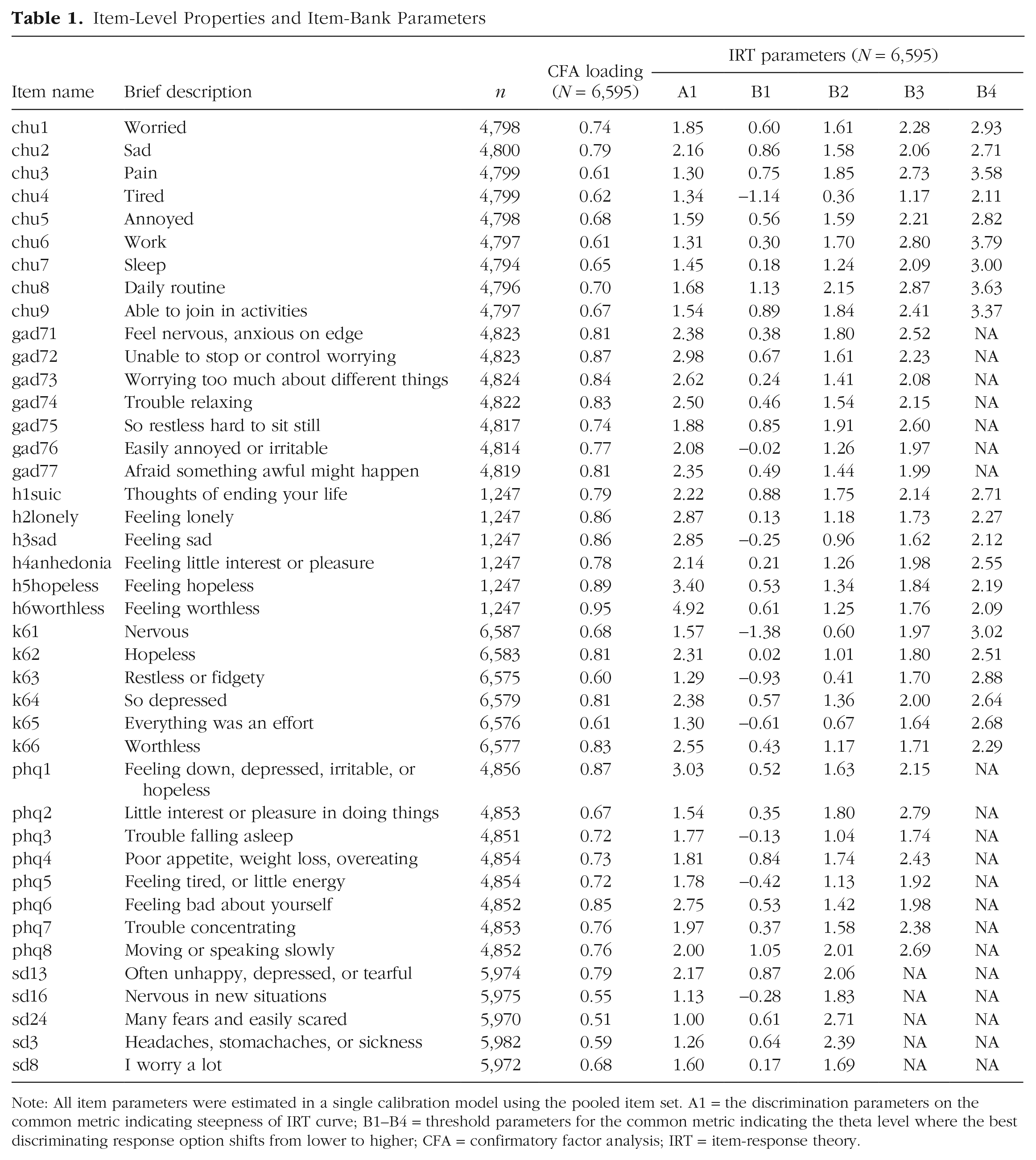
Note: All item parameters were estimated in a single calibration model using the pooled item set. A1 = the discrimination parameters on the common metric indicating steepness of IRT curve; B1–B4 = threshold parameters for the common metric indicating the theta level where the best discriminating response option shifts from lower to higher; CFA = confirmatory factor analysis; IRT = item-response theory.

Item-bank properties

The final item parameters for the total-item pool generated from a single concurrent calibration are provided in Table 1. These parameters can be used to generate common-metric scores using any combination of items included in the total pool. Scores derived from the total-item pool will differ in precision depending on where the individual sits on the underlying dimension. As shown in Figure 1, the total-item pool provides the most precision and therefore the least error for people who exhibit scores in the mid to upper severity levels (greater than −1 to 3 on theta) and relatively little precision for less severe ranges (less than –1 on theta). Note that a value of 0.44 in terms of standard error is equivalent to a reliability of 0.8. Inspection of the standard-error curves using the items that form each of the scales, provided in Figure S1 in the Supplemental Material, indicate differing degrees of precision depending on whether the scores on the common metric were derived using different scales. Common-metric scores derived using the K6, PHQ-8, GAD-7, CHU-9D, and BSI-D provide acceptable level of precision for scores that fall between the −1 and 3 range. Scores on the common metric derived using the SDQ provide relatively less precision at the theta range between −1 and 3 compared with the remaining scales, given a higher standard error.

Fig. 1.

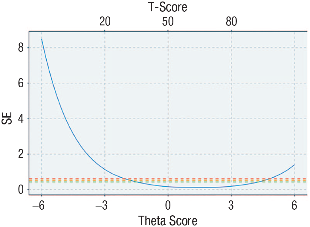
Standard-error curve of full-item bank. Green dashed line represents an equivalent reliability of 0.8, orange dashed line represents an equivalent reliability of 0.7, and red dashed line represents an equivalent reliability of 0.6.

Common-metric crosswalks and interpretation of scores

Easy-to-use crosswalk tables that take sum scores from each of the scales and map them to the equivalent theta and t score on the common metric are displayed graphically in Figure 2 and available in Appendix A in the Supplemental Material. These tables provide a quick indication of the potential common-metric score and associated error. However, this method is somewhat limited in that the same sum score can be generated from different items with different item parameters. Given access to full-response data on the individual items, it is possible to take the item parameters into account and generate individual common-metric scores using the mirt package in R (Chalmers, 2012). An example program is provided in Appendix C in the Supplemental Material. To assist with interpretation of scores on the common metric, curves relating the total sum scores to theta and t scores for each scale are provided in Figure S2 in the Supplemental Material. In addition, published clinical cut points for the PHQ-8, GAD-7, K-6, and SDQ were assessed with respect to the equivalent scores on common metric to identify a “clinical range.” The cut points converged on an area of the common metric ranging between theta scores of 1.17 and 2.02 (or 61.7 and 70.2 in t scores).

Fig. 2.

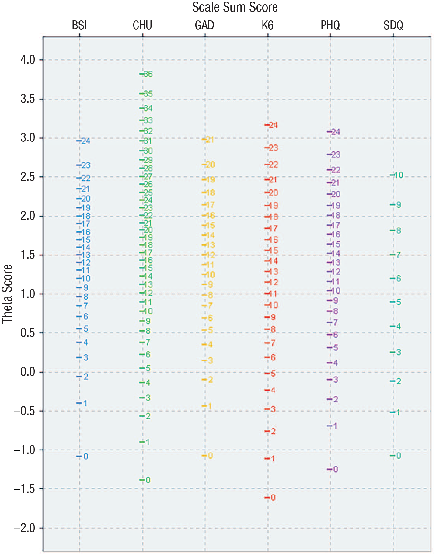
Crosswalk table for sum scores to theta scores for each of the equated scales.

To further assist with interpretation, additional graphs were generated that map the theta and t scores onto the response category with the highest probability of endorsement for each item from all the scales (graphs are provided in Appendix B in the Supplementary Material). These graphs provide a concrete interpretation of the common-metric scores by back translating the scores to what might be expected in terms of responses on the individual items. For example, individuals who score an average score on the common metric (e.g., 0) or lower have the highest probability of endorsing the “not at all” option for each item on the GAD-7 scale. However, we note that back translating theta scores in this manner can contribute increased levels of measurement error, and therefore, we recommend using these maps to aid interpretation of the theta scores rather than for conversion.

The level of agreement between common-metric scores derived from responses from each individual scale compared with common-metric scores derived from all available items is shown in Figure 3 (and Table S6 in the Supplemental Material). ICCs in the validation sample ranged from 0.76 for the SDQ to 0.92 for the BSI-D. The Bland-Altman plots provide some indication that agreement between scores was better at the more severe/clinical range of the common-metric spectrum (i.e., theta scores ranging between 0 and 3), particularly scores derived from the PHQ-8, GAD-7, and BSI-D, and there was evidence of a floor effect across all measures, as is common in measures of psychopathology in general samples.

Fig. 3.

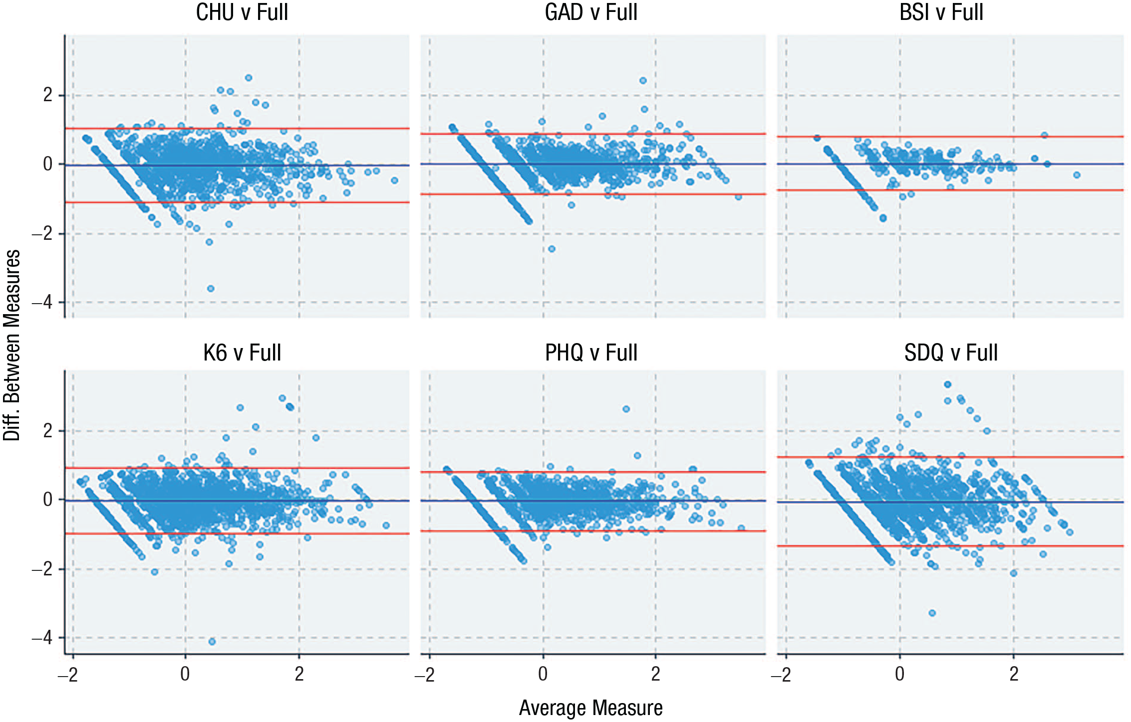
Bland-Altman plots comparing common-metric scores derived from the full-item pool in comparison with common-metric scores derived from individual scales using all available data in the validation sample (n = 1,716).

Discussion

The aim of the current study was to develop a common metric based on existing and widely applied scales to measure symptoms of distress in adolescent samples. In the current study, we equated six scales using an IRT-based equating approach and developed crosswalks to map scores from each scale onto a common metric that offers a standardized interpretation of data across different data sets (and R programs to generate individual scores). The common metric provides scores with acceptable levels of precision across the −1 to 3 range on theta, which equates to the more severe and often clinical end of the spectrum. Indeed, many symptom-based measures in mental health capture the upper severity end of the respective dimensional spectra given the relatively lower prevalence of the symptoms in the general population and the greater interest among clinicians and researchers in targeting clinical or at-risk levels. Thus, the precision level of the common metric at lower, “nonclinical” levels may be insufficient for detailed assessment and monitoring and might be suitable only for broad screening of the population. A clinical threshold was determined by mapping preexisting clinical cut points for the individual scales on the common metric, which converged on similar values ranging between 1.17 and 2.02. These values could be used to inform clinicians that individuals who score at or above this range may require additional follow-up or treatment for depression or anxiety disorders. However, the use of these cut points should be to aid interpretation rather than a formal diagnosis given that the metric is best represented as a continuous dimension to capture more nuanced information rather than categorizing people above or below an artificial threshold.

Further inspection of the standardized factor loadings and the discrimination parameters for the total-item pool indicate that the common metric is best represented by indicators that target hopelessness, depression, and worry. This corresponds to prior evidence indicating that the distress subfactor of the HiTOP model can be best described as representing symptoms of depression, dysthymia, and generalized anxiety (Kotov et al., 2017). The interpretation of the common metric as a distress subfactor may also explain why the precision rates based on items from the CHU-9D and SDQ were relatively worse than those from the GAD-7, PHQ-8, K6, and BSI-D. The CHU-9D was developed as a broad, preference-based, quality-of-life measure for adolescents and includes only three items that target distress with the other items that index physical health and daily functioning (that are moderately related to mental health). Likewise, the SDQ emotionality subscale contains only two items that target depression and worry, whereas the other items index fear-type symptoms such as panic and social anxiety as well as somatization, which have previously been demonstrated as loading on separate but related subfactors in the HiTOP structure. Thus, it could be questioned whether the CHU-9D and SDQ should be incorporated into the current common metric. However, recent studies have demonstrated the utility of using the CHU-9D as a potential mental-health measure in addition to economic evaluations (Furber & Segal, 2015). Given the widespread use of the CHU-9D and SDQ in many routine data collections, the inclusion of these scales potentially enhances the utility of the common metric and may enable greater data comparisons. The choice of additional scales to include on the common metric for the current study was also largely restricted to the availability of data. Future studies could possibly expand on the common metric derived in the current study by using fixed-item calibration methods in new samples that contain at least one of the previously equated scales and the new scale to be included on the common metric. Previous evidence has demonstrated the feasibility of this approach by equating additional scales that measure depression on the PROMIS-depression metric (Kaat et al., 2017).

The results of the current study demonstrate the initial utility of the HiTOP structure as a potential empirical framework to generate a hierarchy of common metrics that can be used to link related scales and data sets. For example, the different levels of the hierarchy could be used to equate broader or more specific sets of scales depending on whether there is interest in scoring broad internalizing, broad distress, or specific disorders/symptoms clusters, such as depression. Other published common metrics in the literature, specifically those targeting depression and social anxiety, have provided more information about the specific syndromes/disorders at the lower levels of the hierarchy (Sunderland et al., 2018; Wahl et al., 2014). Therefore, it might be feasible to use a single scale such as the PHQ-8 to provide two different scores depending on whether the interest is in evaluating the distress subfactor (using item parameters published in this study) or major depressive disorder (using item parameters published in previous work focusing on depression scales).

The current study has many strengths, including the use of two large samples of Australian school-age adolescents to generate the item parameters for a comprehensive set of widely used scales that measure depression and anxiety. However, the study is somewhat limited given the reliance on self-reported data and that the sample was not obtained to be representative of Australian adolescents and does not represent a clinical sample. Likewise, the racial and ethnic identification of the students participating in the study was unknown. Additional validation work is required to ensure the item parameters generated in this population are invariant in clinical populations and can be used to accurately compare clinical cohorts. Likewise, additional work could be conducted by recruiting a representative sample of adolescents and then normalizing the common metric according to the representative population mean, thus providing a more generalizable interpretation of common-metric scores. Finally, the validation and interpretation of the common metric developed in the current study should be examined further in independent samples by inspecting associations with other clinically relevant and theoretically related constructs, such as emotional regulation, neuroticism, and negative cognitive bias.

In summary, in the current study, we identified a coherent common metric that is closely aligned with the distress subfactor of the HiTOP model and captures common variance between symptoms of depression and chronic worry/generalized anxiety in adolescent samples. This metric offers researchers and clinicians a greater level of flexibility to score, combine, and compare different data sets without the requirement of having used consistent measures, moving the field forward in terms of data harmonization to answer important questions that may not be sufficiently answered in any single data set.

Supplemental Material

sj-docx-1-cpx-10.1177_21677026231168564 – Supplemental material for “One Metric to Rule Them All”: A Common Metric for Symptoms of Depression and Generalized Anxiety in Adolescent Samples

Supplemental material, sj-docx-1-cpx-10.1177_21677026231168564 for “One Metric to Rule Them All”: A Common Metric for Symptoms of Depression and Generalized Anxiety in Adolescent Samples by Matthew Sunderland, Nicholas Olsen, Rachel Visontay, Cath Chapman, Louise Mewton, Lexine Stapinski, Nicola Newton, Maree Teesson and Tim Slade in Clinical Psychological Science

Footnotes

Transparency

Action Editor: Jennifer L. Tackett

Editor: Jennifer L. Tackett

Author Contributions

Matthew Sunderland: Conceptualization; Formal analysis; Investigation; Methodology; Visualization; Writing – original draft; Writing – review & editing.

Nick Olsen: Conceptualization; Data curation; Methodology; Writing – review & editing.

Rachel Visontay: Formal analysis; Methodology; Visualization; Writing – review & editing.

Cath Chapman: Conceptualization; Project administration; Writing – review & editing.

Louise Mewton: Conceptualization; Methodology; Writing – review & editing.

Lexine Stapinski: Conceptualization; Data curation; Funding acquisition; Project administration; Writing – review & editing.

Nicola Newton: Conceptualization; Funding acquisition; Project administration; Writing – review & editing.

Maree Teesson: Conceptualization; Funding acquisition; Project administration; Supervision; Writing – review & editing.

Tim Slade: Conceptualization; Data curation; Funding acquisition; Methodology; Supervision; Writing – review & editing.

ORCID iD

Matthew Sunderland

Supplemental Material

Additional supporting information can be found at

References

Andrews

Anderson

T. M.

Slade

Sunderland

(2008). Classification of anxiety and depressive disorders: Problems and solutions. Depression and Anxiety, 25(4), 274–281. https://doi.org/10.1002/da.20489

Andrews

Goldberg

D. P.

Krueger

R. F.

Carpenter

W. T.

Hyman

S. E.

Sachdev

Pine

D. S.

(2009). Exploring the feasibility of a meta-structure for DSM-V and ICD-11: Could it improve utility and validity? Psychological Medicine, 39(12), 1993–2000. https://doi.org/10.1017/S0033291709990250

Batterham

P. J.

Sunderland

Slade

Calear

A. L.

Carragher

(2018). Assessing distress in the community: Psychometric properties and crosswalk comparison of eight measures of psychological distress. Psychological Medicine, 48(8), 1316–1324. https://doi.org/10.1017/S0033291717002835

Buckman

J. E. J.

Saunders

Cohen

Z. D.

Barnett

Clarke

Ambler

Derubeis

R. J.

Gilbody

Hollon

S. D.

Kendrick

Watkins

Wiles

Kessler

Richards

Sharp

Brabyn

Littlewood

Salisbury

White

I. R.

. . . Pilling

(2021). The contribution of depressive ‘disorder characteristics’ to determinations of prognosis for adults with depression: An individual patient data meta-analysis. Psychological Medicine, 51(7), 1068–1081. https://doi.org/10.1017/S0033291721001367

Buckman

J. E. J.

Saunders

Stott

Arundell

L. L.

O’Driscoll

Davies

M. R.

Eley

T. C.

Hollon

S. D.

Kendrick

Ambler

Cohen

Z. D.

Watkins

Gilbody

Wiles

Kessler

Richards

Brabyn

Littlewood

DeRubeis

R. J.

. . . Pilling

(2021). Role of age, gender and marital status in prognosis for adults with depression: An individual patient data meta-analysis. Epidemiology and Psychiatric Sciences, 30, Article e42. https://doi.org/10.1017/S2045796021000342

Cervin

Norris

L. A.

Ginsburg

Gosch

E. A.

Compton

S. N.

Piacentini

Albano

A. M.

Sakolsky

Birmaher

Keeton

Storch

E. A.

Kendall

P. C.

(2021). The p factor consistently predicts long-term psychiatric and functional outcomes in anxiety-disordered youth. Journal of the American Academy of Child & Adolescent Psychiatry, 60(7), 902–912.e5. https://doi.org/10.1016/J.JAAC.2020.08.440

Chalmers

R. P.

(2012). Mirt: A multidimensional item response theory package for the R environment. Journal of Statistical Software, 48(6), 1–29. https://doi.org/10.18637/jss.v048.i06

Choi

S. W.

Gibbons

L. E.

Crane

P. K.

(2011). lordif: An R package for detecting differential item functioning using iterative Hybrid ordinal logistic regression/item response theory and Monte Carlo simulations. Journal of Statistical Software, 39(8), 1–30. https://doi.org/10.18637/jss.v039.i08

Choi

S. W.

Schalet

Cook

K. F.

Cella

(2014). Establishing a common metric for depressive symptoms: Linking the BDI-II, CES-D, and PHQ-9 to PROMIS Depression. Psychological Assessment, 26(2), 513–527. https://doi.org/10.1037/a0035768

10.

Conway

C. C.

Forbes

M. K.

Forbush

K. T.

Fried

E. I.

Hallquist

M. N.

Kotov

Mullins-Sweatt

S. N.

Shackman

A. J.

Skodol

A. E.

South

S. C.

Sunderland

Waszczuk

M. A.

Zald

D. H.

Afzali

M. H.

Bornovalova

M. A.

Carragher

Docherty

A. R.

Jonas

K. G.

Krueger

R. F.

. . . Eaton

N. R.

(2019). A hierarchical taxonomy of psychopathology can transform mental health research. Perspectives on Psychological Science, 14(3), 419–436. https://doi.org/10.1177/1745691618810696

11.

Cook

K. F.

Schalet

B. D.

Kallen

M. A.

Rutsohn

J. P.

Cella

(2015). Establishing a common metric for self-reported pain: Linking BPI Pain Interference and SF-36 Bodily Pain Subscale scores to the PROMIS Pain Interference metric. Quality of Life Research, 24(10), 2305–2318. https://doi.org/10.1007/s11136-015-0987-6

12.

Curran

P. J.

Cole

Giordano

Georgeson

A. R.

Hussong

A. M.

Bauer

D. J.

(2018). Advancing the study of adolescent substance use through the use of integrative data analysis. Evaluation & the Health Professions, 41(2), 216–245. https://doi.org/10.1177/0163278717747947

13.

Derogatis

L. R.

Melisaratos

(1983). The Brief Symptom Inventory: An introductory report. Psychological Medicine, 13(3), 595–605. https://doi.org/10.1017/S0033291700048017

14.

Dorans

N. J.

(2007). Linking scores from multiple health outcome instruments. Quality of Life Research, 16(Suppl. 1), 85–94. https://doi.org/10.1007/s11136-006-9155-3

15.

Dunn

T. J.

Baguley

Brunsden

(2014). From alpha to omega: A practical solution to the pervasive problem of internal consistency estimation. British Journal of Psychology, 105(3), 399–412. https://doi.org/10.1111/bjop.12046

16.

Farber

Wolpert

Kemmer

(2020). Common measures for mental health science. Laying the foundations. https://wellcome.org/sites/default/files/CMB-and-CMA-July-2020-pdf.pdf

17.

Forbes

M. K.

Sunderland

Rapee

R. M.

Batterham

P. J.

Calear

A. L.

Carragher

Ruggero

Zimmerman

Baillie

A. J.

Lynch

S. J.

Mewton

Slade

Krueger

R. F.

(2021). A detailed hierarchical model of psychopathology: From individual symptoms up to the general factor of psychopathology. Clinical Psychological Science, 9(2), 139–168. https://doi.org/10.1177/2167702620954799

18.

Fried

E. I.

(2017). The 52 symptoms of major depression: Lack of content overlap among seven common depression scales. Journal of Affective Disorders, 208, 191–197. https://doi.org/10.1016/J.JAD.2016.10.019

19.

Furber

Segal

(2015). The validity of the Child Health Utility instrument (CHU9D) as a routine outcome measure for use in child and adolescent mental health services. Health and Quality of Life Outcomes, 13(1), 1–14. https://doi.org/10.1186/s12955-015-0218-4

20.

Gatz

Reynolds

C. A.

Finkel

Hahn

C. J.

Zhou

Zavala

(2015). Data harmonization in aging research: Not so fast. Experimental Aging Research, 41(5), 475–495. https://doi.org/10.1080/0361073X.2015.1085748

21.

Gibbons

R. D.

Perraillon

M. C.

Kim

J. B.

(2014). Item response theory approaches to harmonization and research synthesis. Health Services and Outcomes Research Methodology, 14(4), 213–231. https://doi.org/10.1007/s10742-014-0125-x

22.

Goodman

(2001). Psychometric properties of the strengths and difficulties questionnaire. Journal of the American Academy of Child and Adolescent Psychiatry, 40(11), 1337–1345. https://doi.org/10.1097/00004583-200111000-00015

23.

L. T.

Bentler

P. M.

(1998). Fit indices in covariance structure modeling: Sensitivity to underparameterized model misspecification. Psychological Methods, 3(4), 424–453.

24.

Hyland

Murphy

Shevlin

Bentall

R. P.

Karatzias

G. W. K.

Boduszek

McElroy

(2021). On top or underneath: Where does the general factor of psychopathology fit within a dimensional model of psychopathology? Psychological Medicine, 51(14), 2422–2432. https://doi.org/10.1017/S003329172000104X

25.

Kaat

A. J.

Kallen

M. A.

Nowinski

C. J.

Sterling

S. A.

Westbrook

S. R.

Peters

J. T.

(2020). PROMIS® pediatric depressive symptoms as a harmonized score metric. Journal of Pediatric Psychology, 45(3), 271–280. https://doi.org/10.1093/JPEPSY/JSZ081

26.

Kaat

A. J.

Newcomb

M. E.

Ryan

D. T.

Mustanski

(2017). Expanding a common metric for depression reporting: Linking two scales to PROMIS® depression. Quality of Life Research, 26, 1119–1128. https://doi.org/10.1007/s11136-016-1450-z

27.

Karyotaki

Efthimiou

Miguel

Bermpohl

F. M. G.

Furukawa

T. A.

Cuijpers

Riper

Patel

Mira

Gemmil

A. W.

Yeung

A. S.

Lange

Williams

A. D.

Mackinnon

Geraedts

Van Straten

Meyer

Björkelund

Knaevelsrud

. . . Forsell

(2021). Internet-based cognitive behavioral therapy for depression: A systematic review and individual patient data network meta-analysis. JAMA Psychiatry, 78(4), 361–371. https://doi.org/10.1001/JAMAPSYCHIATRY.2020.4364

28.

Kessler

R. C.

Andrews

Colpe

L. J.

Hiripi

Mroczek

D. K.

Normand

S. L. T.

Walters

E. E.

Zaslavsky

A. M.

(2002). Short screening scales to monitor population prevalences and trends in non-specific psychological distress. Psychological Medicine, 32(6), 959–976. https://doi.org/10.1017/S0033291702006074

29.

Kim

S. H.

Cohen

A. S.

(2016). A comparison of linking and concurrent calibration under the graded response model. Applied Psychological Measurement, 26(1), 25–41. https://doi.org/10.1177/0146621602026001002

30.

Kim

S. H.

Cohen

A. S.

Alagoz

Kim

(2007). DIF detection and effect size measures for polytomously scored items. Journal of Educational Measurement, 44(2), 93–116. https://doi.org/10.1111/j.1745-3984.2007.00029.x

31.

Kolen

M. J.

Brennan

R. L.

(2014). Test equating, scaling, and linking (3rd ed.). Springer.

32.

Kotov

Krueger

R. F.

Watson

Achenbach

T. M.

Althoff

R. R.

Bagby

R. M.

Brown

T. A.

Carpenter

W. T.

Caspi

Clark

L. A.

Eaton

N. R.

Forbes

M. K.

Forbush

K. T.

Goldberg

Hasin

Hyman

S. E.

Ivanova

M. Y.

Lynam

D. R.

Markon

. . . Zimmerman

(2017). The hierarchical taxonomy of psychopathology (HiTOP): A dimensional alternative to traditional nosologies. Journal of Abnormal Psychology, 126(4), 454–477. https://doi.org/10.1037/abn0000258

33.

Kroenke

Strine

T. W.

Spitzer

R. L.

Williams

J. B. W.

Berry

J. T.

Mokdad

A. H.

(2009). The PHQ-8 as a measure of current depression in the general population. Journal of Affective Disorders, 114(1–3), 163–173. https://doi.org/10.1016/j.jad.2008.06.026

34.

Krueger

R. F.

(1999). The structure of common mental disorders. Archives of General Psychiatry, 56(10), 921–926. https://doi.org/10.1001/archpsyc.56.10.921

35.

Lawrence

Johnson

Hafekost

Boterhoven De Haan

Sawyer

Ainley

Zubrick

S. R.

(2015). The mental health of children and adolescents: Report on the second Australian child and adolescent survey of mental health and wellbeing [Issue report]. https://www.health.gov.au/sites/default/files/documents/2020/11/the-mental-health-of-children-and-adolescents_0.pdf

36.

Maydeu-Olivares

Joe

(2014). Assessing approximate fit in categorical data analysis. Multivariate Behavioral Research, 49(4), 305–328. https://doi.org/10.1080/00273171.2014.911075

37.

McElroy

Belsky

Carragher

Fearon

Patalay

(2018). Developmental stability of general and specific factors of psychopathology from early childhood to adolescence: Dynamic mutualism or p-differentiation? Journal of Child Psychology and Psychiatry and Allied Disciplines, 59(6), 667–675. https://doi.org/10.1111/jcpp.12849

38.

Mewton

Kessler

R. C.

Slade

Hobbs

M. J.

Brownhill

Birrell

Tonks

Teesson

Newton

Chapman

Allsop

Hides

McBride

Andrews

(2016). The psychometric properties of the Kessler Psychological Distress Scale (K6) in a general population sample of adolescents. Psychological Assessment, 28(10), 1232–1242. https://doi.org/10.1037/pas0000239

39.

Mossman

S. A.

Luft

M. J.

Schroeder

H. K.

Varney

S. T.

Fleck

D. E.

Barzman

D. H.

Gilman

DelBello

M. P.

Strawn

J. R.

(2017). The Generalized Anxiety Disorder 7-item scale in adolescents with generalized anxiety disorder: Signal detection and validation. Annals of Clinical Psychiatry, 29(4), 227–234A.

40.

Muthen

L. K.

Muthen

B. O.

(2017). Mplus User’s Guide (8th ed.). Muthen & Muthen.

41.

Olino

T. M.

McMakin

D. L.

Forbes

E. E.

Seeley

J. R.

Lewinsohn

P. M.

Pilkonis

P. A.

(2013). Comparisons across depression assessment instruments in adolescence and young adulthood: An item response theory study using two linking methods. Journal of Abnormal Child Psychology, 41(8), 1267–1277. https://doi.org/10.1007/S10802-013-9756-6/TABLES/3

42.

Patalay

Fried

E. I.

(2021). Editorial perspective: Prescribing measures: Unintended negative consequences of mandating standardized mental health measurement. Journal of Child Psychology and Psychiatry and Allied Disciplines, 62(8), 1032–1036. https://doi.org/10.1111/jcpp.13333

43.

Ratcliffe

Huynh

Chen

Stevens

Swait

Brazier

Sawyer

Roberts

Flynn

(2016). Valuing the Child Health Utility 9D: Using profile case best worst scaling methods to develop a new adolescent specific scoring algorithm. Social Science & Medicine, 157, 48–59. https://doi.org/10.1016/j.socscimed.2016.03.042

44.

Ringwald

W. R.

Forbes

M. K.

Wright

A. G. C.

(2021). Meta-analysis of structural evidence for the Hierarchical Taxonomy of Psychopathology (HiTOP) model. Psychological Medicine. Advance online publication. https://doi.org/10.1017/S0033291721001902

45.

Rodriguez

Reise

S. P.

Haviland

M. G.

(2016). Evaluating bifactor models: Calculating and interpreting statistical indices. Psychological Methods, 21(2), 137–150. https://doi.org/10.1037/met0000045

46.

Rothrock

N. E.

Amtmann

Cook

K. F.

(2020). Development and validation of an interpretive guide for PROMIS scores. Journal of Patient-Reported Outcomes, 4(1), Article 16. https://doi.org/10.1186/s41687-020-0181-7

47.

Samejima

(1997). Graded response model. In Linden

W. J.

Hambleton

R. K.

(Eds.), Handbook of modern item response theory (pp. 85–100). Springer. https://doi.org/10.1007/978-1-4757-2691-6_5

48.

Schalet

B. D.

Cook

K. F.

Choi

S. W.

Cella

(2014). Establishing a common metric for self-reported anxiety: Linking the MASQ, PANAS, and GAD-7 to PROMIS anxiety. Journal of Anxiety Disorders, 28(1), 88–96. https://doi.org/10.1016/j.janxdis.2013.11.006

49.

Schalet

B. D.

Revicki

D. A.

Cook

K. F.

Krishnan

Fries

J. F.

Cella

(2015). Establishing a common metric for physical function: Linking the HAQ-DI and SF-36 PF subscale to PROMIS® physical function. Journal of General Internal Medicine, 30(10), 1517–1523. https://doi.org/10.1007/s11606-015-3360-0

50.

Schalet

B. D.

Rothrock

N. E.

Hays

R. D.

Kazis

L. E.

Cook

K. F.

Rutsohn

J. P.

Cella

(2015). Linking physical and mental health summary scores from the veterans RAND 12-item health survey (VR-12) to the PROMIS® global health scale. Journal of General Internal Medicine, 30(10), 1524–1530. https://doi.org/10.1007/s11606-015-3453-9

51.

Shin

Lee

S.-H.

Han

K.-M.

Yoon

H.-K.

Han

(2019). Comparison of the usefulness of the PHQ-8 and PHQ-9 for screening for major depressive disorder: Analysis of psychiatric outpatient data. Psychiatry Investigation, 16(4), 300–305. https://doi.org/10.30773/PI.2019.02.01

52.

Slade

Watson

(2006). The structure of common DSM-IV and ICD-10 mental disorders in the Australian general population. Psychological Medicine, 36(11), 1593–1600. https://doi.org/10.1017/S0033291706008452

53.

Spitzer

R. L.

Kroenke

Williams

J. B. W.

Löwe

(2006). A brief measure for assessing generalized anxiety disorder: The GAD-7. Archives of Internal Medicine, 166(10), 1092–1097. https://doi.org/10.1001/archinte.166.10.1092

54.

Sunderland

Batterham

Calear

Carragher

Baillie

Slade

(2018). High agreement was obtained across scores from multiple equated scales for social anxiety disorder using item response theory. Journal of Clinical Epidemiology, 99, 132–143. https://doi.org/10.1016/j.jclinepi.2018.04.003

55.

Teesson

Newton

N. C.

Slade

Carragher

Barrett

E. L.

Champion

K. E.

Kelly

E. V.

Nair

N. K.

Stapinski

L. A.

Conrod

P. J.

(2017). Combined universal and selective prevention for adolescent alcohol use: A cluster randomized controlled trial. Psychological Medicine, 47(10), 1761–1770. https://doi.org/10.1017/S0033291717000198

56.

Teesson

Newton

N. C.

Slade

Chapman

Birrell

Mewton

Mather

Hides

McBride

Allsop

Andrews

(2020). Combined prevention for substance use, depression, and anxiety in adolescence: A cluster-randomised controlled trial of a digital online intervention. The Lancet Digital Health, 2(2), e74–e84. https://doi.org/10.1016/S2589-7500(19)30213-4

57.

Thissen

Pommerich

Billeaud

Williams

V. S. L.

(1995). Item response theory for scores on tests including polytomous items with ordered responses. Applied Psychological Measurement, 19(1), 39–49. https://doi.org/10.1177/014662169501900105

58.

Wahl

Löwe

Bjorner

J. B.

Fischer

Langs

Voderholzer

Aita

S. A.

Bergemann

Brähler

Rose

(2014). Standardization of depression measurement: A common metric was developed for 11 self-report depression measures. Journal of Clinical Epidemiology, 67(1), 73–86. https://doi.org/10.1016/j.jclinepi.2013.04.019

59.

Wolpert

(2020). Funders agree first common metrics for mental health science. LinkedIn. https://www.linkedin.com/pulse/funders-agree-first-common-metrics-mental-health-science-wolpert/

60.

Levis

Riehm

K. E.

Saadat

Levis

A. W.

Azar

Rice

D. B.

Boruff

Cuijpers

Gilbody

Ioannidis

J. P. A.

Kloda

L. A.

McMillan

Patten

S. B.

Shrier

Ziegelstein

R. C.

Akena

D. H.

Arroll

Ayalon

. . . Thombs

B. D.

(2020). Equivalency of the diagnostic accuracy of the PHQ-8 and PHQ-9: A systematic review and individual participant data meta-analysis. Psychological Medicine, 50(8), 1368–1380. https://doi.org/10.1017/S0033291719001314

Supplementary Material

Please find the following supplemental material available below.

For Open Access articles published under a Creative Commons License, all supplemental material carries the same license as the article it is associated with.

For non-Open Access articles published, all supplemental material carries a non-exclusive license, and permission requests for re-use of supplemental material or any part of supplemental material shall be sent directly to the copyright owner as specified in the copyright notice associated with the article.

0.00 MB

0.40 MB