Testing Predicted Clusters

Abstract

Testing predicted clusters of questionnaire items can be a source of abundant feedback on the theory that is behind the prediction. Such testing is often performed by means of confirmatory factor analysis. However, that method offers insufficient feedback at the level of items, while its goodness-of-fit indices are notoriously unreliable. Richer and more precise feedback would be generated by a data-driven optimization of the predicted clusters (factors), allowing a comparison between predicted and empirical clusters (factors) at the level of items. Contrasting these two provides a basis for classifying the items into hits, false positives, and false negatives. This division greatly facilitates reinterpretation of the clusters (factors) and evaluation of the items. In addition, it offers a basis for two new measures of goodness of fit with respect to the correct assignment of items to clusters (indicators to factors). Application of this new approach to a questionnaire on Obsessive–Compulsive Disorder will serve as an illustration of its merits for both a qualitative and quantitative evaluation of the predicted clusters.

Keywords

factor testing goodness of fit construct validation factor comparison obsessive–compulsive disorder

Introduction

Testing predicted clusters of variables, for instance, within a psychopathological category, is a powerful tool in theory development because a multitude of expected correlations is tested in one hit. Seeing these variables cluster in line with a priori theoretical ideas is strong support for these, while deviations from the predicted clustering provide detailed feedback that can help modify the theory. At the same time, this approach can serve as construct validation of multidimensional questionnaires in psychology and related disciplines.

This raises three questions: (a) How can we arrive at empirical item clusters that correspond to the predicted clusters to make a comparison both possible and useful? This question is addressed in the next two sections. (b) How can we evaluate the discrepancies between predicted and empirical clustering at the level of individual items? What output will provide the kind of feedback that is both detailed and useful? These questions are treated in “Qualitative comparison of predicted and empirical clusters” section. (c) How can we estimate the goodness of fit (GOF) between the predicted and empirical clusters with a single, clear-cut measure, preferably a number between 0 and 1? Two new measures are proposed in “A measure for the accuracy of cluster prediction in terms of items” and “A second measure in terms of factor loadings (or item-cluster correlations [ICC])” sections.

To avoid misunderstandings, certain points of view and concepts in this article are clarified in advance; they represent the position taken up by the author: (a) Collecting information about a multitude of variables simultaneously is typically done by means of tests and questionnaires. This article confines itself to questionnaires in the realm of clinical and personality psychology; it does not address capacity or aptitude tests. (b) Because the article is about questionnaires, the term items is used instead of (observed) variables. (c) Questionnaire items are viewed here as variables on interval scales, not ordinal scales, even though it is more realistic to consider the strength of such variables as lying in between ordinal and interval levels. (d) The relationship between variables is expressed in product-moment correlations, but the methods and measures discussed may be applicable to other correlation coefficients as well. (e) To avoid circumstantial language in discussing the topics of this article, it is assumed that there are no variables to be reflected or that they have already been reflected before the correlation matrix was calculated. (f) Questionnaire items, such as those representing a diagnostic category in psychopathology, are considered imperfect representations of behavioral and experiential phenomena in the form of judgments about these. They are not considered “measurements” of so-called latent variables, as is the assumption in confirmatory factor analysis (CFA). However, this does not deny that the clustering will be affected by various “latent variables” (e.g., personality characteristics). (g) Factor analysis is considered a group of methods to detect and identify item clusters. Factors represent these clusters. A factor label is a phrasing of the common denominator of an item cluster, not the name of its cause. A factor is something to be explained—it does not explain anything in and of itself.

CFA and Its Limitations

CFA is often the first choice when researchers want to test a predicted factor structure in a multidimensional measurement instrument or other set of observed variables. CFA is executed by means of structural equation modeling, a procedure to test complex theoretical models, rooted in common factor analysis. In CFA, the clusters of items within a test or questionnaire are interpreted as consisting of the indicators (anchor items) of the factors, while the factors are interpreted as “latent variables,” explaining the clustering of the indicators.

CFA tests predictions about the measurement part of the model. The model always specifies the indicator-factor relations, often whether the factor structure is orthogonal or oblique, and whether there will be cross-loadings. When the structure is expected to be oblique, a hierarchical factor model may be predicted. Sometimes, the unique variances of the variables are predicted to correlate. All of these relations constitute the parameters of the model. The predicted parameters are fixed (constrained); the remaining parameters are left free to be estimated. Sufficient parameters should be fixed to make the model identifiable.

These predictions are translated into a simplified covariance matrix over all of the observed variables, with an estimation of the communalities in the diagonal. This matrix is then adjusted by means of maximum likelihood estimation or another algorithm in a number of iterations to the empirical covariance matrix. This results in the implied covariance matrix. This latter matrix is subtracted from the empirical matrix, which results in the residual matrix. If the residuals are sufficiently small—to be judged by means of χ² (which should show that both matrices do not differ significantly) and some measures of “goodness of fit” (GOF indices)—the prediction is considered to hold for both the sample and the population.

Limitations: Insufficient information at the item level

Such an all-or-none decision, however, may not be the only or main issue in which the researcher is interested. Especially in the early and intermediate phases of his investigation, one may prefer more detailed feedback, which enables improvement of the theory or test, or both (Anderson & Gerbing, 1988). The global estimates of GOF in CFA do not show where the prediction errors are located.

More informative feedback would be provided by a factor structure with factors that correspond to the predicted factor structure in number and nature, on the one hand, and that are in good agreement with the empirical covariance or correlation matrix,¹ on the other. CFA, however, produces a factor structure that is strongly affected by the implied correlation matrix. In this structure, secondary factor loadings are lacking if they had been fixed at zero in the prediction, and most or all of them are. Thus, the investigator can see which items have a suspiciously low primary loading but not whether these items had been better reallocated to another factor or whether they cross-load on another factor.

The output also includes modification indices per parameter. These indices show to what extent χ² and one or more of the GOF indices could adopt a better value by modifying predictions. The researcher can “free” the fixed parameter with the poorest value, have it estimated by the iterative procedure mentioned earlier, and fix it anew or one could fix a parameter that had been left free. One could continue this freeing and fixing until there is a very good fit, but then the model tested is no longer the model predicted.

Problems with GOF

When CFA is applied to the measurement model in an advanced stage of research, all primary factor loadings and modification indices may seem good enough, χ² may be nonsignificant, and the GOF indices may have favorable values. Can the predicted cluster structure now be unconditionally trusted to be confirmed? No, it cannot. For the past 15 years, several studies have demonstrated that both χ² and the GOF indices are heavily affected by incidental parameters, obscuring the effect of the predicted parameters. Prudon (2015) provided an overview that can be supplemented by the research of Savalei (2012) who confines herself to the GOF index root mean square error of approximation. Conclusions are that (a) GOF is erroneously indicated to be poor if the factor loadings are high and to be good when they are low; (b) GOF is erroneously estimated as good if there are many factors in proportion to the number of indicators; and (c) when the factors correlate relatively highly but their correlation has been left free for estimation, overlooked cross-loadings are not easily detected. This is an avoidable, but not often avoided, omission by the researcher.

Incorrect assignment of indicators to factors is another instance of model misspecification. It is the most critical one and is central to this article. CFA’s suitability to detect this kind of misspecification was investigated by Stuive (2007) and her team (Stuive, Kiers, & Timmermans, 2009; Stuive, Kiers, Timmermans, & ten Berge, 2008). They found that the degree of unique variance (which affects the height of the factor loadings) had a highly obscuring influence on the detection of assignment errors, especially in combination with a high factor correlation (.70) that had not been fixed in the model.

Cluster Optimization as an Entrance to Testing Predicted Clusters

As stated earlier in “Limitations: insufficient information at the item level” subsection, what is needed in the analysis of the clustering of variables is a reconstitution of the predicted factor structure in good agreement with the empirical correlation matrix. Comparing the predicted factor structure with such an optimized one will provide the best feedback, but how to arrive at such a result?

Procrustes rotation

One could perform an exploratory factor analysis (EFA) with the instruction to draw only the predicted number of factors and perform an oblique rotation. However, EFA may be overly affected by accidental or spuriously high correlations. This would be the case, for instance, if some items were very similar. It may also be distorted by an excess of items belonging to a certain cluster or by a rather high correlation between two clusters that, according to the prediction, should be kept distinct. So, there is an insufficient guarantee that the acquired factor structure is continuous with the predicted factor structure.

A possible means to obtain such a factor structure could be a Procrustes rotation (a forced rotation) of the factors obtained by EFA for maximum similarity with a target factor structure, that is, the predicted factors (Digman, 1967; Schönemann, 1966; Van de Vijver & Leung, 1997). Presently, however, Procrustes rotation for the sake of factor structure testing has been overshadowed by CFA; few studies can be found that use it.

Model respecification by means of CFA

CFA contains the option to respecify a model with mediocre fit, as described in the “Limitations: insufficient information at the item level” subsection. This procedure can be continued until optimal fit is reached. Stuive (2007) and her team (Stuive et al., 2009) undertook such enterprise in two studies with simulated data. Assignment errors were introduced in a 3 × 4 items test, as mild error = one item in the wrong subtest and moderate error = two subtests had an item exchanged. In a 3 × 6 items test an additional, supposedly graver, error was introduced: two items of Subtest A were assigned to Subtest B; one item of B was assigned to A. These partly incorrect factor structures were optimized by CFA, executed by means of LISREL. Best results were seen when no stopping criteria were applied.

In both studies, the true factor structure was discovered in 100% of the cases with the milder assignment error and in 95% to 100% of the cases with the gravest assignment error. This held if the unique variance was set on 20% or 50% and was true even for the smaller sample sizes. Thus, the respecification by means of CFA performed well, at least for this simple structure with only 12 or 18 test items. However, with real data, more variables, graver assignment errors, and the application of stopping criteria, the results might become less favorable.

MacCallum, Roznowski, and Necowitz (1992) have criticized such drastic model respecification because it runs a high risk of capitalizing on chance. This concept means that the new model will be adjusted to all whims of the data, including sample imperfections and fluctuations, in the first place, and also errors in data gathering, suboptimal test construction, and so on. On a new sample, such an extremely respecified model may show a mediocre fit once again. However, that would only be a problem if the respecified factor structure is to be adopted unconditionally, but that is not the purpose of the respecification in this case. Here, it serves merely to compare a predicted factor structure with an empirical factor structure that is molded to this predicted structure. This empirical factor structure will certainly be imperfect, it will be dependent on the sample, and it will not be the only possible one that could be imposed on the available data. Nonetheless, it generates much more feedback on the prediction than that in the regular output of CFA. However, applying stopping criteria as thresholds to avoid model respecification on the basis of minor deviations is recommendable.

Exploratory structural equation modeling

The earlier subsection shows that CFA can also be used to find a factor structure that is much more in line with the empirical correlation matrix than the predicted factor structure. Still, the forced zero value of all or most secondary factor loadings is unrealistic and uninformative; in addition, it spuriously increases the factor correlations (Marsh et al., 2010, p. 485). However, in 2009, Asparouhov and Muthén introduced a variant of CFA, called exploratory structural equation modeling (ESEM). This approach was intended to overcome the aforementioned limitations of CFA. In this method, in addition to a CFA measurement model, an EFA measurement model with rotations can be used within a structural equation model. There is no longer a need to fix the nonindicators per factor at 0. They can be freely estimated, and they are reproduced in the output.

The superiority of ESEM to CFA in cases of more complex measurement models has already been demonstrated in studies such as Marsh et al. (2010), Furnham, Guenole, Levine, and Chamorro-Premuzic (2013), Booth and Hughes (2014), and Guay, Morin, Litalien Valois, and Vallerand (2014). ESEM can be used very well for a data-driven model respecification, resulting in a much more realistic and informative factor structure than CFA.

Multiple group method of factoring

An older type of factor analysis, the multiple group method, may also be suited to test and optimize predicted factors. This method was proposed, more or less independently and simultaneously, by Holzinger (1944), Guttman (1944), and Thurstone (1945). The brief account given here follows Holzinger (1944).

Divide the correlation matrix into sections (i.e., groups of highly correlating variables) beforehand. Transform these clusters into factors by means of matrix–algebraic formulas. These initial factors will usually stand in an oblique relation to one another. Calculate a reproduced correlation matrix over the variables (a correlation matrix, inferred from the factor structure). Subtract this reproduced matrix from the empirical correlation matrix; this results in a residual correlation matrix. If the residuals are close to 0, the factoring is considered successful. In the case of many large residuals, however, an additional factor, orthogonal to the extant ones, could be extracted. An alternative would be to resection the residual correlation matrix to secure a better fit. (Holzinger did not explain how to do the latter.)

The sectioning of the correlation matrix beforehand could be based on the empirical correlations but also on theoretical grounds. Guttman (1952) appeared to be a proponent of such an approach. In such a case, the multiple group method of factoring is akin to CFA but with the advantage of producing an EFA-like factor structure. The original impetus for this preclustering of the correlations was to save computation time in the pre-computer era. That goal has been superseded, but the theory-testing possibilities of the multiple group method may be a reason for renewed attention to it. A good starting point for this enterprise could be Harman’s discussion of the method (Harman, 1976, pp. 234–243).

Stuive and her team claimed to have applied the multiple group method of factoring to test (Stuive et al., 2008) and optimize (Stuive et al., 2009) predicted factors, calling it the oblique multiple group method. However, their description of this procedure shows that it is actually an example of the method described later.

Optimizing Clusters Iteratively Based on Item Analysis (Predicted Cluster Optimization)

The procedure given here is the one used in the examples in this article. For this reason, it is described in a separate section in more detail. However, it must be stressed that this article is not meant as a defense of or plea for this specific method but only as a plea for optimizing predicted clusters (by whatever method) to compare the optimized with the predicted ones. The method in question is item analysis within the tradition of classical test theory, that is, on the basis of correlations between the items and their test scale. To distinguish it from item analysis within the framework of item response theory, it will be denoted here as correlative item analysis (CIA).

CIA involves calculating the correlations between all test items and all (sub)test scales of the test concerned. The test scale score is usually represented by the unweighted sum (or mean) of the raw item scores of the scale.² (Sub)test scales will further be denoted as clusters. The item-cluster correlations of the items assigned to that cluster have to be corrected for self-correlation. This can be done by temporarily subtracting the item score of concern from the cluster score while the correlation is calculated, this is called item-rest correlation (IRC). The item-cluster correlations of the items not assigned to that cluster will be designated here by the abbreviation ICC.

Among test designers, CIA is applied to improve a test under construction in the following way: An item that correlates far too low with its own cluster is deleted or is reallocated to another cluster with which it sufficiently correlates, provided the move makes sense. If more than a few items are to be (re)moved, CIA should be performed both very gradually (from larger errors to smaller errors) and iteratively (Stouthard, 2006) because after each modification, the whole picture of ICCs of the clusters concerned changes. When applied in this way, CIA appears to offer a first-rate opportunity for the optimization of predicted clusters in accordance with the empirical correlation matrix. However, the procedure will differ from that of test designers in two ways:

If test designers are applying CIA, they will be strongly steered by substantive considerations about the item content and scale interpretation. They will, therefore, be less systematic, less exhaustive, and less radical in item reallocations than what is to be recommended for theory testing. Polishing and fine tuning their instrument is all they need; minor deviations from what should theoretically be the ICCs are considered normal and not a reason for further modifications. This, however, is not the procedure to be advocated in the case of cluster optimization for the purpose of theory testing. The optimization, then, is to be steered and terminated by purely quantitative considerations and criteria. It has to be not only systematic but also radical and exhaustive, apart from certain thresholds. The eventual cluster structure will undoubtedly be strongly capitalized on chance and other undesirable factors (McCallum et al., 1992), but it will be in close accordance with the empirical correlation matrix on the one hand and show continuity with the predicted clusters on the other.

Test designers may be quick to delete modestly correlating items to improve the homogeneity of the subscales. They may also remove highly correlating items if these no longer increase Cronbach’s alpha, just for the sake of parsimony. And they may discard highly cross-loading items to improve the distinctness of their test scales. Here, too, the interests of the theory-testing researcher are opposite: no items should be discarded. Whether clustered or nonclustered, differently clustered than predicted, having poor IRC’s or high ones, having high correlations with other clusters or not, they all provide feedback on the theory behind the cluster prediction and feedback on the quality of the items. (Once this feedback has been processed, the researcher may, of course, proceed with deleting or reformulating items for the sake of improving the questionnaire.)

Because of all of these differences with the way CIA is executed for the sake of test construction, the procedure advocated here will be granted its own label: predicted cluster optimization (PCO).³

Such purely quantitative optimization may sound simpler than it is. A number of decisions have to be made, including (a) when to consider an IRC sufficiently high for its cluster (e.g., ≥ .40); (b) how much homogeneity and parsimony one should consider desirable; and (c) what thresholds on reallocation are necessary and what values they should be given. Some inconvenient arbitrariness in such decisions is unavoidable. However, further discussion of this issue is beyond the scope of this article.⁴

Example of Qualitative Comparison of Predicted With Empirical Clusters: Obsessive–Compulsive Disorder

PCO yields well-circumscribed clusters of items. This enables the researcher to compare predicted with empirical clusters at the level of items and ICCs. ESEM starts from well-circumscribed clusters (the indicators), but the optimized ones will be clear-cut only after a cutoff value for factor loadings has been specified to distinguish indicators from nonindicators per factor. When that issue has been solved, the predicted factors can be compared with the empirical ones.

This comparison specifies which items the predicted clusters have in common with the corresponding empirical ones. These correct positives will be called hits (H-items). Predicted items that end up in a different cluster or that become nonclustered count as false positives (F-items). Items that become member of a cluster unexpectedly can be considered false negatives, in other words, missing items (M-items). The first concern is to process the H-, F-, and M-items at a qualitative level. What type of output will provide a practical feedback? This will be discussed on the basis of an example: a PCO⁵ on a questionnaire for Obsessive–Compulsive Disorder (OCD).

From 1974 until 1981, a colleague and I ran a research project on OCD at the University of Nijmegen, the Netherlands. OCD impressed me as a heterogeneous condition. To explore this issue, I drafted a questionnaire of 108 items for self-rating that should capture the various typical obsessive–compulsive phenomena. Items were rated on 5-point scale ranging from 1 (Does not apply to me) to 5 (Applies to me completely). Based on case studies, the OCD literature, and theoretical notions, I devised items for five expected clusters:

Cluster 1. Contamination anxiety, washing compulsion, “dirt” avoidance.

Cluster 2. Other unrealistic worries (e.g., having harmed people unawares), unrealistic behavior (e.g., rituals to prevent harm).

Cluster 3. Obsessions: unacceptable thoughts, images, and impulses (e.g., aggressive and obscene).

Cluster 4. Clinging to subordinate behaviors (e.g., tidiness and checking) as a simplistic means to cope with difficult problems in living; feeling dissatisfied with such behavior without knowing why.

Cluster 5. Disintegration: a complete lapse into subordinate and trivial behavior.

A developmental disorder in the differentiation of the behavioral repertoire was hypothesized to be at the basis of Clusters 1 and 2, which were thus expected to correlate positively. A developmental disorder in the integration of the behavioral repertoire was supposed to underlie both Clusters 4 and 5. In addition, Cluster 4 behavior could eventually disintegrate and then assume characteristics of Cluster 5 phenomena. Thus, Clusters 4 and 5 were expected to correlate highly. An obstructed development of the emotional and assertive behavioral repertoire was thought to be a breeding ground of obsessions.

The items of the five clusters were more or less equally distributed over the questionnaire. A sample of 43 in- and out-patients with a primary diagnosis of OCD and a sample of 52 nonclinical subjects, matched on sex, age, and education, rated themselves on the items. Most items appeared to be highly discriminating between both groups, so the questionnaire was relied upon to measure OCD. To investigate the hypothesized heterogeneity, only the patients with OCD were used. Four doubtful cases were excluded to avoid attenuating the clustering by a large number of low scores. The supposed heterogeneity of OCD was presumed to guarantee sufficient distribution of the item scores for a sound correlation matrix. The small number of participants (39) was, of course, disproportional to the number of items, but studying the clustering of the items was nevertheless expected to be informative. Whether reliable or not, the results allow for an illustration of the proposed approach to cluster testing.

Three problematic items were rejected beforehand (one double, one overlapping, and one ill-formulated) and eight items were rejected afterwards because of insufficient score distribution (SD < 1.0).⁶ The correlation matrix was calculated for all items. For this matrix, the five predicted clusters (minus the rejected items) were tested with a crude manual version of PCO. The results were reported in Prudon (1981). For the sake of this article, the data were reanalyzed with a refined computerized version of PCO, and its results are presented here.⁷ The final clusters (except Cluster 1) deviated greatly from the predicted ones, not surprising in this early stage of the research. They demanded a considerable refinement of the theoretical notions, but not their rejection.

A global and quick impression of what happened to the preclustering of the items (in the recent analysis) can be gained from Table 1. In this table, the predicted items are divided into hits and false positives, while the final clusters include missing items, next to the hits. Items with high cross-correlations with another cluster are specified in the rightmost column; behind them in brackets are the “rival” clusters. (An arbitrary and perhaps too small difference of ≤ .05 was used as a criterion for high cross-correlations.)

Table 1.

Qualification of the Predicted Items in Terms of Hits, False Positives, and Missing (N = 39).

Cluster	Cp	Cf	H-items	F-items	M-items	CC-items
1	15	14	1 5 9 13 54 58 62 66 70 74 82 86 106 107	50		74 (4) 74 (5)
2	13	13	17 21 29 90 94 98 108	25 33 37 101 103 104	19 23 26 39 50 72
3	21	18	3 7 11 15 27 34 45 47 60 64 68 88 92	19 23 26 39 52 72 80 84	12 16 33 101 103	34 (2) 64 (4)
4	17	12	2 6 10 14 18 51 59 63 67 71 75	22 55 79 91 95 99	28	22 (5) 51 (5)
5	31	32	8 20 24 32 36 40 42 43 44 46 49 57 65 69 73 77 81 85 89 93 96 97	4 12 16 28 38 48 53 61 100	22 25 37 52 55 79 91 95 99 104	8 (4) 36 (4) 37 (4) 40 (4)

Note. Cp = number of items in the predicted cluster; Cf = number of items in the final, optimized cluster; CC items = highly cross-correlating items (difference IRC-ICC < .05; between brackets: the “rival” cluster). Eight nonclustered items: 4 38 48 53 61 80 84 100. Three rejected items in advance: 35 78 102; eight because SD < 1.0: 30 31 41 56 76 83 87 105.

Table 1 shows that Clusters 2 and 3 exchanged several items. Cluster 4 passed several items to the related Cluster 5, but Cluster 5 only passed one to Cluster 4. Consequently, the common denominator of Cluster 4 had to be narrowed to “cleaning, clearing and ordering as simplistic means to cope with complicated problems in living.” More serious prediction errors involved the reallocation of items to unrelated clusters: three Cluster 2 items (25, 37, and 104) went to Cluster 5 despite a correlation of −.29 between the two clusters; and two Cluster 5 items (12 and 16) went to Cluster 3 despite the independence of these two clusters (correlation −.03). Six F-items from Cluster 5 remained nonclustered.

The cluster correlations are reproduced in Table 2. The correlation between Clusters 1 and 2 was confirmed, as was as the high correlation between Clusters 4 and 5. The moderate positive correlation between Clusters 2 and 3 is probably due to the shared harming theme; that between Clusters 3 and 4 is not so obvious. The cluster characterizations in the right-hand column are based on their revised interpretation, not the expected one.

Table 2.

Cluster Correlations Between the Optimized Clusters (N = 39).

Cluster	1	2	3	4	Cluster characterization
1					Contamination anxiety (being harmed in diffuse ways)
2	+.46				Fear of unintentionally harming other people in diffuse ways
3	+.07	+.36			Obsessions, often about explicit harm to close others
4	+.09	−.04	+.36		Ordering, clearing, and cleaning compulsion
5	−.11	−.29	−.03	+.61	Compulsive precision, checking, and ritualizing (disintegration)

Practical Output for Qualitative Cluster Comparison at the Level of Items

To understand why this item exchange took place and to estimate what reinterpretation of the clusters it necessitated, we must look at the content of the F- and M-items, in relation to the content of the H-items. Useful to this goal is a table in the output in which the item content can be inserted. This table can be sorted according to the predicted cluster number and the final cluster number. The resulting tables comprise the missed items, the hits, and the false items, with each category arranged according to the ICCs from high to low. Table 3 serves as an illustration of this output and its helpfulness.

Table 3.

Item and Cluster Interpretation of Cluster 2 With the Help of a Table, Sorted on f, p, and IRC.

		p	f	IRC	ICC	Chr.
	M-items
50	Aware of risk of contaminating others with germs, therefore much washing.	1	2	.66	.62 p = .00	dhm
41r	Idea that unawares I took something valuable that wasn’t mine.	3	2	.31	.13 p > .05	dhm
39	Idea that indirectly I may be the cause of harm to someone else.	3	2	.83	.30 p < .04	negl
26	Afraid someone may have accident with things I handled last, so I take pains to leave them safe.	3	2	.75	.34 p < .02	dhm, negl
72	Urge to check the fire, gas, sockets, and so on, at home, to make sure nobody will be harmed.	3	2	.71	.36 p < .02	negl
19	Idea that gas-supply or stove in room house-mate is in no good condition so that he may be killed.	3	2	.69	.49 p = .00	negl
23	Idea that I may have left pins, thumbtacks, splinters, and so on, at somebody’s place.	3	2	.68	.06 p > .05	dhm
105r	When I learn of accidents or fires somewhere, I worry it may be my fault.	3	2	.36	.01 p > .05	dhm
76r	I check the papers or news to find out whether I may have caused accidents or fires somewhere.	3	2	.32	.15 p > .05	dhm
	Hits
108	When I see a stone and so on, lying in the street, I often feel someone may stumble over it which would be my fault.	2	2	.76	.31³ p < .03	negl
94	I watch for dangerous objects in the street and remove these to protect my fellow-man.	2	2	.69	.25¹ p > .05	negl
98	I push aside glass and pebbles in the street because they might hurt others, which would be partly my fault.	2	2	.67	.35³ p < .02	negl
90	In the street I look behind me to check if I have unawares caused accidents.	2	2	.66	.23¹ p > .05	dhm
29	I feel someone may stumble over a stone if I was the last one who touched it.	2	2	.65	.38¹ p < .01	dhm
17	I feel I carry dangerous things (e.g., fire) with me, causing disasters somewhere.	2	2	.62	.35¹ p < .02	dhm
21	Afraid I haven’t quite extinguished my cigarette-stubs, so things may catch fire.	2	2	.55	.12¹ p > .05	dhm
	F-items (sorted on p and f, instead of f and p)
33	When I have a malicious thought I am often afraid it will actually come true.	2	3	.75	.27 p < .05	taf
103	I worry about unlikely dangers besetting me.	2	3	.63	.31 p < .03	–
101	Sinful deed or thought compels me to do or say a special thing, to “wipe it out.”	2	3	.55	.29 p < .04	mag
104	To assure a certain event will pass off well, I have to perform a particular action.	2	5	.53	.06 p > .05	mag
25	I often feel, unawares, I may have done stupid things, with disastrous consequences.	2	5	.45	−.02 p > .05	dhm
37	Before going to bed or going out, and so on, I am afraid things may cause accidents, so I have to check everything carefully.	2	5	.45	.16 p > .05	negl

Note. p = item predicted to belong to the cluster below; f = item belonging to the final cluster; IRC = correlation of the item with the final cluster; ICC = correlation of the item with the predicted cluster, but in the case of a hit the next highest correlation (in superscript the cluster concerned); Chr. = characterization of the item: dhm = direct, diffuse harm; negl = harm by negligence; taf = thought–action fusion; mag = magically averting danger. An r behind the item number in the most left column indicates it was a rejected item (while IRC ≥ .30). The probability of ICC is directional.

Cluster 2 is chosen for Table 3 because it had the poorest prediction, but its optimization nevertheless made sense. For reasons of convenience, the items are rephrased in brief style. To assist in the reinterpretation of the clusters, a seventh column is added at the utmost right side with a coded characterization of the item (symbol “Chr.”). The items that were rejected because of their small SD are also included to determine whether they would have clustered in line with the prediction and what could be the reason for their small SD.

Reinterpretation of Cluster 2 Based on Table 3

The original interpretation of Cluster 2 was “instances of unrealistic ideas (e.g., far-fetched worries of having harmed other people) and idem behavior (e.g., rituals to prevent harm).” What could be the reinterpretation?

First, let us look at the seven hits. The first three involve concerns about being indirectly responsible (by one’s negligence) for harm that befalls one’s fellow man, despite this responsibility being of a very remote, far-fetched nature. The last four hits pertain to worries of having done harm to one’s fellow man in a direct way or running the risk of doing so. However, the way this harm might have been inflicted, or may be inflicted, is poorly specified, remains vague, or seems even magical. In sum, these seven items represent a person’s feeling of being able to harm another person without consciously willing so and without the intervention of any explicit action or deliberate neglect. Such a feeling motivates the patient to engage excessive, bizarre attempts at verifying and preventing the harm imagined.

Now let us have a look at the missed items. All but one came from the predicted Cluster 3, “Obsessions.” Most of these items also refer to harming other people. However, in the reallocated items, the culpability is said to be of an indirect, poorly specified, or far-fetched nature. This feature they share with the hits in Cluster 2. The items that remained in Cluster 3 appear to refer to a more explicitly inflicted, direct harm: intrusive thoughts, images or impulses of a violent, aggressive, rebellious, or obscene nature. The one remaining missing item in final Cluster 2 (Item 50) came from Cluster 1 (contamination anxiety and washing compulsion). It refers to active contamination fear: “I will contaminate, and thus harm, other persons.” This appears to be just another instance of a diffuse, uncontrollable, and unintentional way of harming people.

Thus, unrealistic thinking and behaving as such is not the common denominator of Cluster 2; instead, it is the poorly specified, often indirect way in which an imagined harm could have been, or could be, inflicted. Fantasies of moral reprehensibility surround these worries.

Why did the six false positives of the predicted Cluster 2 not fit into the final Cluster 2? In Item 33, the harming is not of a diffuse nature but is instead felt to be a magical consequence of an explicit, malicious thought; Item 101 refers to an obsession about explicit harm; Item 104 does not refer to an idea of (diffusely) harming people. Item 103, rather instead, refers to obsessive ruminating rather than harming in an unrealistic way. Items 25 and 37 were reinterpreted at the time as instances of fear of showing incompetence (“under-effectiveness”), in line with the incompleteness experience that is part of Clusters 5 and 4, rather than of causing harm in a diffuse way (“over-effectiveness”).

An obvious limitation of the study discussed is the small sample, which increases the risk of not being representative and of instability of the correlations. In addition, I endorsed the revised Cluster 2 completely at the time because all reallocations seemed to make sense. Perhaps a more conservative approach is to be recommended, considering the results of a recent investigation with a revised version of this questionnaire on a larger sample (N = 105). In this new sample, Items 25 and 37 appeared to be better at home in Cluster 2 than in Cluster 5, in accordance with the original prediction!

However, that is not what is at stake here. The previous sections serve only as an illustration of the richness of the feedback stemming from a detailed comparison of predicted and corresponding empirical clusters (factors). It shows what kind of output would be practical in reinterpreting one’s results. Tables such as Table 3 allow for a detailed and systematic comparison of predicted and final clusters, which will facilitate the revision of one’s theoretical notions or of one’s questionnaire. If only the theoretical notions are revised, then a new cluster prediction could be based on it that is closer to the empirical cluster structure. However, it must be stressed again that the revised prediction need not be identical to the optimized one: The prediction should be theoretically defensible. If not, the revision could be nothing but capitalization on chance and on various methodological imperfections.

The investigator could try out this new cluster prediction on the same sample, but this will probably only result in a smaller, yet not nullified discrepancy with the empirical clusters. The scientific community will be more convinced by the results on a new sample. Such cross-validation is necessary anyway if the questionnaire has been revised.

A Measure for Accuracy of Cluster Prediction in Terms of Items

The division of the predicted items in terms of the hits, false positives, and missing items is also the point of departure for measuring the accuracy of the prediction of cluster membership (indicator assignment) in the following way. The number of H-, F-, and M-items is specified. These numbers will be expressed by the variables H, F, and M, respectively. Each such item is given a weight of 1. Now, the following formula in terms of H, F, and M is reasonably obvious (it is the 12th of a series of dissimilarity coefficients between binary variables, as presented by Gower & Legendre, 1986⁸)

AP (it) = \frac{H}{\sqrt{(H + F) . (H + M)}}

Formula 1 (tentative)

This index, AP(it), which means “Accuracy of Prediction (in terms of items),” will range from 1 (perfect fit) to, theoretically, 0 (no hits). Let us call the number of items in the predicted cluster Cp and the number of items in the final cluster Cf. Because Cp = H + F and Cf = H + M, the formula can be simplified to the following

AP (it) = \frac{H}{\sqrt{Cp . Cf}}

Formula 2 (tentative)

However, in this formula, the number of hits by chance, which could have been scored by random assignment, has not yet been accounted for. For example, if 30 items are dispersed over three clusters that are defined by 10 items each, the chance of scoring a hit is 1 in 3. That chance implies 3.33 hits on 10 items. A perfect prediction will still result in an AP(it) of 1, but a random distribution will not result in an AP(it) of 0. Therefore, a correction for chance must be added to the formula. If the total number of items that are allowed to participate in the analysis is k, then the Cp items have a chance of Cp /k to be assigned to the final cluster. The final cluster consists of Cf items; thus, Cp.Cf/k items will be a hit on the basis of mere chance

p (H) = \frac{Cp . Cf}{k}

Formula 3 (final)

When added to Formula 2, the following formula results

AP (it) = \frac{H - p (H)}{\sqrt{(Cp - p (H)) . (Cf - p (H))}}

Formula 4 (final)

If the prediction does not exceed the level of mere guessing, then this time, AP(it) will be 0. In the case of a perfect prediction, it will still be 1. If one deliberately “predicts” below chance level, then AP(it) will even become negative. Unlike the GOF-indices, AP(it) is independent of the average level of item-correlations and ICCs because it is in terms of true–false, 1–0.

Table 4 is suited to calculate AP(it). It is based on the assignment errors that are used in the simulation study by Stuive et al. (2009), which was discussed in “Model re-specification by means of confirmatory factor analysis” subsection. Remember that in Study 1, a test with three subscales of four items each was used. The mild error was that one item from Subtest B went to Subtest A; the moderate error was that A and B exchanged one item. In Study 2, three subtests of six items were used. The same prediction errors as in Study 1 were introduced, and a third, supposedly “graver,” error was involved: Two items of Subtest A had been assigned to Subtest B, and one item of B had been assigned to A. The mildest error of Study 2 is ignored in Table 4.

Table 4.

AP(it) in the Simulation Studies of Stuive et al. (2009).

Cluster	Study 1: Mild error							Study 1: Moderate error
Cluster	Cp	H	F	M	Cf	p(H)	AP(it)	Cp	H	F	M	Cf	p(H)	AP(it)
A	5	4	1	0	4	1.67	0.84	4	3	1	1	4	1.33	0.63
B	3	3	0	1	4	1.00	0.82	4	3	1	1	4	1.33	0.63
C	4	4	0	0	4	1.33	1.00	4	4	0	0	4	1.33	1.00
Total or mean	12	11	1	1	12	4.00	0.88	12	10	1	1	12	4.00	0.75
	Study 2: “Moderate” error							Study 2: “Graver” error
A	6	5	1	1	6	2.00	0.75	5	4	1	2	6	1.67	0.61
B	6	5	1	1	6	2.00	0.75	7	5	2	1	6	2.33	0.64
C	6	6	0	0	6	2.00	1.00	6	6	0	0	6	2.00	1.00
Total or mean	18	16	2	2	18	6.00	0.83	18	15	3	3	18	6.00	0.75

Note. Cp = number of items in the factor as predicted; Cf = number of items in the factor after optimizing; H = hits, number correctly assigned items; F = number of falsely assigned items; M = number of items missed in the assignment; p(H) = number of items which might have been correctly assigned by chance; AP(it) = accuracy of the prediction in terms of items.

The AP values give a convenient impression of the gravity of the assignment errors. Note that the “moderate error” is less erroneous in Study 2 than in Study 1, while the so-called graver error in Study 2 is just as grave as the moderate error in Study 1. This finding shows that AP(it) is suitable to assess the gravity of the assignment errors in advance, if one wants to apply CFA on simulated data. It can also be used in empirical studies with CFA after the predicted factors have been respecified based on the modification indices.

Note further that every cluster prediction has its own AP(it); thus, it is more informative than the GOF indices in CFA, but it is also possible to add up H, F, M, and p(H) over the three clusters to calculate an average AP(it) over the cluster prediction as a whole.

A Second GOF Index in Terms of ICCs (or Factor Loadings)

AP(it) depends on a strict distinction between the hits, false items, and missing items. However, a false positive that nevertheless has a relatively high correlation with the cluster from which it has been expelled could be regarded as a lesser mistake than one that has a very low or even negative correlation with that abandoned cluster. On the other hand, a missing item that has a relatively low correlation with the final cluster toward which it has been moved is a smaller error than a missing item that has a high correlation with its final cluster.

How could the formula be adjusted to do justice to these divergent ICCs? A solution would be to no longer attach a weight of 1 to the hits, false, and missing items, but a weight that depends on their ICC or factor loading, as the case may be.⁹ As follows:

(a) H could be substituted by the sum of the factor loadings of the H-items: ΣLdH. The index of this ∑ ranges from 1 to H, but is not shown in the formulas.

(b) Likewise, M is to be substituted by the sum of loadings on M-items, ΣLdM, in which the index of ∑ ranges from 1 to M.

Analogously to H + M = Cf, the following holds: ΣLdH + ΣLdM = ΣLdCf. The index of ΣLdCf ranges from 1 to Cf. H + F = Cp, however, cannot simply be replaced by ΣLdH + ΣLdF = ΣCp. The reason is that this action would imply punishing instead of rewarding for high loadings of F-items (which, remember, is the milder error). This issue can be solved by assigning each F-item a weight that rests on the difference between the average loading of the final factor and the loading of the F-item: $\bar{L} dCf$ − LdF. In the AP(it) formula, F has now to be replaced by F.( $\bar{L} dCf$ − LdF) = F. $\bar{L} dCf$ − ΣLdF). Note that $F . \bar{L} dCf$ can be replaced by $\frac{F}{Cf} \cdot \sum LdCf$ .

Now, Formula 2 can be transformed into Formula 5, in which AP(ld) stands for “Accuracy of prediction in terms of factor loadings.” In the case of ICCs, AP(icc) should be used.

Formula 5 (tentative) : AP (ld) = \frac{\sum LdH}{\sqrt{(\sum LdH + \frac{F}{Cf} . \sum LdCf - \sum LdF) . \sum LdCf}}

However, here too, a correction for chance is to be incorporated into the formula, this time in terms of factor loadings. Remember, the number of items of the final cluster that could have been predicted correctly merely by chance equals $Cp . Cf / Cp . Cf k k$ (see “A measure for the accuracy of cluster prediction in terms of items” section, Formula 3). In this chance correction, the term Cp/k can be retained without modification, but Cf has to be replaced by the weighted sum $\sum LdCf$ . Thus, the total weight of the hits by chance would be the following

p (\sum LdH) = \frac{Cp}{k} . \sum LdCf

Formula 6 (final)

Formula 5 can now be transformed into Formula 7, which includes the chance correction, p(ΣLdH)

Formula 7 (final) : AP (ld) = \frac{\sum LdH - p (\sum LdH)}{\sqrt{(\sum LdH - p (\sum LdH) + \frac{F}{Cf} . \sum LdCf - \sum LdF}) . (\sum LdCf - p (\sum LdH))}

When the missing items in the optimized factor have the same mean loading as the hits, while the F-items have a mean loading of 0, then AP(ld) will equal AP(it). If, under these conditions, the F-items have on average a negative loading, then AP(ld) will be somewhat lower than AP(it). In all of the other cases, AP(ld) will be more or less higher than AP(it). For a systematic account of the behavior of AP(ld) in relation to AP(it), consult Table A1 in Appendix A. It will also show that AP(ld) is independent of the average height of the factor loadings, unlike the GOF indices of CFA.

Table A1.

Values of AP(it) and AP(ld) Under Different Conditions.

Note that this weighted AP cannot be used when the cluster optimizations have been executed by CFA because (almost all) the secondary factor loadings are absent in the output of CFA.

Application of the Two Measures to the Example

Original study (1981)

At this point, it is interesting to see how AP(it) and AP(icc)¹⁰ can be used to evaluate the prediction in the empirical study that was discussed in “Qualitative comparison of predicted with empirical clusters” section. The values of CP, H, F, M, and Cf can be derived from Table 1. The ICCs can be inspected via the link http://home.kpn.nl/p.prudon/OCD-output-brief.pdf. The dependent variables can be calculated from these data. The results of comparing the predicted with the final, optimized clusters are shown in Table 5. For the sake of convenience, the critical dependent variables AP(it) and AP(icc) have been printed in boldface.

Table 5.

Comparison of Predicted With Optimized Clusters in the Questionnaire on OCD (Prudon, 1981).

Cluster	Independent variables							Dependent variables
Cluster	Cp	H	F	M	Cf	p(H)	p(Hl)	AP(it)	AP(icc)	Coh.p	Coh.f	α
1. Contamination	15	14	1	0	14	2.16	1.54	.96	.99	.52	.53	.940
2. Diffuse harm	13	7	6	6	13	1.74	1.20	.47	.48	.21	.50	.929
3. Obsessions	21	13	8	5	18	3.90	2.20	.59	.64	.21	.34	.904
4. Cleaning etc.	17	11	6	1	13	2.10	1.38	.73	.83	.35	.47	.913
5. Disintegration	31	22	9	10	31	10.23	5.83	.55	.61	.18	.31	.935
Total or weighted mean	97	67	30	22	89	20.13	12.15	.636	.689			.926

Note. OCD = Obsessive–Compulsive Disorder; Cp = number of items in the predicted cluster (= H + F); H = number of hits, correctly assigned items; F = number of false positives; M = number of items missed in cluster prediction; Cf = number of items in the final cluster (= H + M); p(H) = number of hits, assigned by chance; p(Hl) = $p (\sum LdH) =$ weighted sum of hits (weight depending on mean factor loading, or item-cluster correlation, as is the case here); AP(it) = accuracy of prediction in terms of items; AP(icc) = accuracy of prediction in terms of item-cluster correlations of the items; Coh. = cohesion, mean inter-item correlation per cluster (p = predicted; f = final); α = Cronbach’s alpha of the final clusters; Weighted mean = weight depends on Cf. Eleven items out of 108 were rejected; eight items became nonclustered. For abbreviated Cluster labels, see Table 2.

Observation of Table 5 indicates that (a) only Cluster 1 was predicted almost perfectly (APs of .96 and .99, respectively); (b) Cluster 2 scored poorly (APs of .47 and .48, respectively) for reasons explained in “Reinterpretation of Cluster 2 by means of Table 3” subsection; (c) Cluster 3 had a somewhat better prediction (APs of .59 and .64, respectively); (d) Cluster 4 had several false positives but only one false negative, so it scored rather well with APs of .73 and .83, respectively. The large distance between AP(it) and AP(icc), furthermore, indicated that the F-items had relatively high correlations with the cluster, which means that they were not seriously mistaken; (e) Cluster 5 retained 22 of its 31 items and scored APs of .55 and .61, respectively. On the whole, except for the easy-to-predict Cluster 1, the predictions varied from rather poor to reasonable and required a corresponding degree of revision.

The predicted and optimized clusters can also be compared with respect to their cohesion, defined as the average inter-item correlation of the cluster. The difference shows the degree to which the cluster has gained or lost homogeneity as a consequence of the optimization process, but this only adds information if the corresponding start and final cluster have sufficient items in common.

Table 5, finally, also shows the values of Cronbach’s alpha for the optimized clusters. These values are displayed because alpha is useful for an honest evaluation of the cluster: it weighs the cluster’s size against its homogeneity. Because of the small sample, alpha should not be considered a reliability estimate in this study. The weighted means of AP and alpha give an overall impression of success in cluster prediction. Weighting takes place by multiplying the values of these variables with the sizes of the corresponding final clusters, adding up these products, and dividing them by the total number of items over all final clusters.

Replication study (2014)

The diverse dependent variables in Table 5 also allow for a quick and brief comparison of the results of the original study with those of a replication study. This replication was performed with a revised and extended version (117 items) of the questionnaire of 1981. The prediction of the clusters was in line with the interpretation of the final clusters in the 1981 study. The test was filled out by in- and out-patients all over the country that were suspected by their therapist¹¹ to suffer from (comorbid) OCD. Most of them were not (yet) formally diagnosed as OCD patients. Sixteen of 121 patients scored very low and their scores were no longer used. The raw item scores of the remaining 105 patients were generally lower than those in the 1981 study. Consequently, SD ≥ 1 had to be eased to SD ≥ 0.5 to give Cluster 2 (which counted 10 out of 19 items with an SD < 1.0) a fair chance of reappearing. The results are summarized in Table 6.

Table 6.

Comparison of Predicted With Optimized Clusters in the Revised Questionnaire on OCD (2014).

Cluster	Cp	H	F	M	Cf	p(H)	p(Hl)	AP(it)	Ap(icc)	Coh.p	Coh.f	α
1	14	14	0	4	18	2.17	1.43	.86	.87	.47	.46	.938
2	19	12	7	6	18	2.95	1.56	.58	.74	.33	.32	.894
3	19	15	4	7	22	3.60	1.72	.68	.72	.19	.25	.877
4	16	16	0	1	17	2.34	1.36	.97	.98	.37	.36	.906
5	48	36	12	2	38	15.72	8.09	.76	.86	.22	.26	.929
Total or mean	116	93	23	20	113			.762	.834			.911

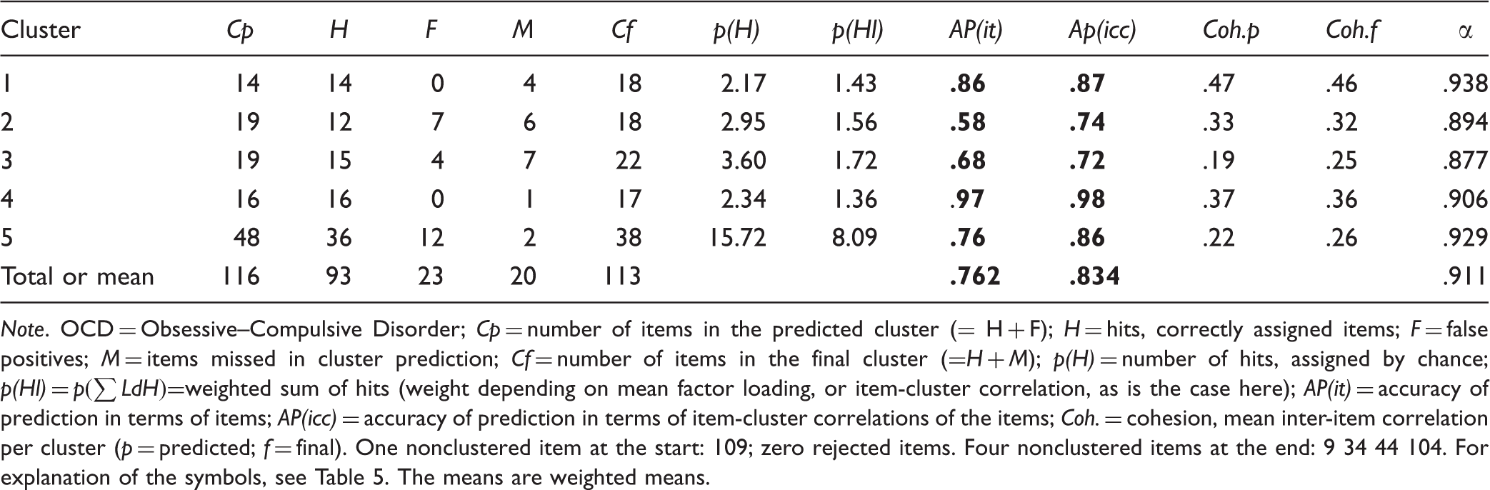
Note. OCD = Obsessive–Compulsive Disorder; Cp = number of items in the predicted cluster (= H + F); H = hits, correctly assigned items; F = false positives; M = items missed in cluster prediction; Cf = number of items in the final cluster (=H + M); p(H) = number of hits, assigned by chance; p(Hl) = $p (\sum LdH)$ =weighted sum of hits (weight depending on mean factor loading, or item-cluster correlation, as is the case here); AP(it) = accuracy of prediction in terms of items; AP(icc) = accuracy of prediction in terms of item-cluster correlations of the items; Coh. = cohesion, mean inter-item correlation per cluster (p = predicted; f = final). One nonclustered item at the start: 109; zero rejected items. Four nonclustered items at the end: 9 34 44 104. For explanation of the symbols, see Table 5. The means are weighted means.

The results for AP are generally better than in 1981. Only Cluster 1 scored worse because the four items about active contamination fear had been assigned to Cluster 2 (see “Reinterpretation of cluster 2 by means of Table 3” subsection) and this was not confirmed by the data. This also yielded four additional F-items in Cluster 2. The APs of both clusters would otherwise have been 1.0 and .69, respectively. In addition, a few items about harm-related checking moved from Cluster 5 to Cluster 2 (in the 1981 study, it was the other way around!).

The homogeneity (cluster cohesion) of the final clusters was less than in 1981, and optimization did not improve it in the case of Clusters 1, 2 and 4. The alphas for Clusters 2 and 3 were lower than in 1981. The neat cluster correlation structure of the 1981 study (see Table 2) was not replicated (not shown here).

The final clusters in the replication might have been closer to the final clusters of the 1981 study, if the sample had consisted of patients with an independent primary diagnosis of OCD. What is at stake here, however, are not the ills and virtues of the questionnaire, theory, or sample, but the suitability of the proposed way of testing cluster (factor) prediction and the related measures of GOF. In this respect, the two examples seem to be good advocates of both.

Interpretation of AP

How much fit do the various values for both APs indicate? To broaden the basis for a tentative interpretation, the present author undertook a number of PCOs on different start clusters, using the data of the original study. Its correlation matrix appeared to be suited to that job because it showed a clear but somewhat complex cluster structure.

What APs would be produced by the optimization of random start clusters? To make the results comparable to those of the original study, the start clusters were given the same sizes as the predicted clusters then. Eight trials were needed to obtain six completed optimizations; two failed because the smallest cluster got emptied. Only once (in Trial 2) did the original five final clusters reappear in almost exactly the same size and composition. In the other trials, the final clusters were highly variable in both size and composition, while some of the cluster correlations were suspiciously high (>.70). Table 7 contains the AP(it)s of the six successful trials. The order of the cluster numbers does not imply corresponding results over the trials, and it does not correspond to that in the original study except in Trial 2, where the cluster numbers were reordered for the sake of comparability.

Table 7.

Comparing the AP’s of Six Trials With PCO on Random Start Clusters.

Cluster	Cp	Cf	AP(it) in 6 trials, original cluster sizes
Cluster	Cp	Cf	1	2X	3	4	5	6
1	15	x	.10	−.02	−.01	.28	.09	.16
2	13	y	.15	.11	.14	.12	.09	.11
3	21	z	.28	.08	.23	.13	.23	.26
4	17	u	.08	.26	.22	.26	.30	.50
5	31	v	.09	.20	.35	.26	.10	.24
Weighted mean	AP(it)		.132	.137	.201	.203	.195	.241
Weighted mean	AP(icc)		.159	.155	.236	.242	.222	.290

Note. PCO = predicted cluster optimization; AP = accuracy of prediction; 2X = original final clusters reappeared almost exactly. The individual AP(icc)s per trial were not reproduced. Weighted mean AP: weight depending on Cf. Cf = x–v: the number of items per final cluster was highly variable.

In Trial 6, the AP(it) of Cluster 4 had a value of .50, which is better than the poorest AP(it) in the original study (Cluster 2), but the other AP(it)s were ≤.35 and two were negative. The weighted average AP(it) per trial ranged from .132 to .241, while the weighted AP(icc)s ranged from .155 to .290.

The values of AP for the random start clusters mentioned earlier, however, are not a realistic baseline. Even lay people who have little or modest psychological knowledge would succeed in ordering the items much above randomness. Nevertheless, these AP values could help somewhat to interpret AP. Table 8 contains a tentative qualification. AP(it) and AP(icc) are treated alike, even though AP(icc) is mostly somewhat higher than AP(it), especially in an oblique cluster structure.

Table 8.

Tentative Characterization of the Degree of Fit Indicated by AP(it) and AP(icc).

0.95–1.00	Model correct; try to estimate whether it may hold for the population as well
0.90–0.94	Model almost correct. Try to ascertain whether this is due to sample fluctuations or whether a minor model revision is necessary
0.80–0.89	Model very well predicted, but it may need some revision
0.70–0.79	Model well predicted, but needs minor to moderate revision
0.60–0.69	Mediocre to reasonable model; needs fair-sized to moderate revision
0.50–0.59	Model has a good core, but is poorly predicted and needs moderate to substantial revision
0.40–0.49	Model still makes some sense, but contains severe misspecifications
0.35–0.39	Model insufficiently predicted, barely above mere guessing. Investigate whether the few hits are interpretable as a valid starting point for interpreting the optimized clusters and whether this interpretation is in line with the guiding idea in the prediction.
<0.35	Poor prediction, probably completely wrong; guiding idea probably to be dismissed

Note. AP(it) = accuracy of prediction in terms of items; AP(icc) = accuracy of prediction in terms of item-cluster correlations of the items.

The qualifications in the table are not to be applied mechanically. The proper work is the inspection of the output on the item level, where it is decided whether the deviations from the prediction are interpretable. A substantial number of assignment errors could suddenly make sense by a minor revision of the theory, whereas one or two misspecified items could remain puzzling or turn out to be detrimental to the theory.

Discussion

The APs appear to perform well at providing a summary evaluation of one’s cluster (factor) predictions. They seem sensitive to even minor imperfections in this prediction. How do they compare to χ² and the GOF indices in CFA and ESEM?

Are Measures of Global Fit Preferable?

The APs give an estimation of the correctness of the allocation of items to clusters, but they are unaffected by misspecified factor correlations, overlooked or misspecified cross-loadings, and correlated residuals. The GOF indices of CFA and ESEM are affected by all of these simultaneously. Is this a reason to prefer the latter? No, because a measure of global fit is highly uninformative: It does not tell which type of prediction errors has been made in which parameters. A global measure may be of use only in SEM, in which there are a few well-established indicators per factor and where the interest is in testing a complex structural model. Moreover, it is not necessary. Cross-loadings and factor correlations are part of the output of ESEM and PCO. So, why not check them directly? A separate AP measure could be devised for them, if deemed useful.

In CFA and ESEM, overlooking unpredicted correlated residual covariances or correlations counts as an instance of misfit. It may be called into question whether this is also justified when large clusters are tested because, then, subclusters within a cluster are a natural and desirable phenomenon. However, insofar it is justified, a way could be found to detect and evaluate such misfit separately. Even if it would be desirable that all of these prediction errors are to be combined into a single measure of fit, then χ² and the GOF indices are unsuitable because they are too much affected by incidental parameters, as argued before (“Problems with goodness of fit” subsection).

Measuring Correct Indicator-Factor (Item-Cluster) Allocation

If the misfit to be detected is an incorrect item-cluster (indicator-factor) allocation, then the APs have a clear advantage over χ² and the GOF indices for the following reasons:

They have a much more transparent origin and are easily interpretable.

They give an impression of the GOF for each cluster (factor) separately (unlike CFA) as well as for the cluster structure (factor structure or pattern) as a whole (like CFA).

The APs are indifferent to the average height of the IRCs (factor loadings) as shown in Appendix A. χ² and the GOF indices of CFA, on the other hand, show artificially good fit when the factor loadings are generally low, leading to the acceptance of incorrect models, whereas they show poor fit when these are generally high, which leads to the rejection of correct models.

The APs are unbiased by the number of clusters (factors) and variables per cluster (factor), unlike some GOF indices.

Unlike χ² and some GOF indices, the APs are unbiased by sample size. CFA and its GOF indices, moreover, need large samples for reliable results. The APs are not dependent on large samples for a good operation. However, this consideration does not deny that they will be more reliable when calculated on larger samples.

The APs have a better range than the GOF indices: They can assume all values between slightly below 0 to exactly 1. The GOF indices, in practice, have a much smaller range. That tiny range would not be a problem if their absolute value could be relied upon (because, then, one could simply stretch the scale), but that is not the case. In contrast, the values of AP are independent of such conditions.

Procrustes rotation of factors was discussed in the eponymous section. In this approach, congruence coefficients are often employed to measure similarity between the factors before and after Procrustes rotation (Harman, 1976, pp. 341–346). The question is: Is factor similarity a good operationalization of correct indicator-factor prediction? If so, a well-known congruence coefficient such as Tucker’s Congruence Coefficient (TCC; Tucker, 1951) could be a valid alternative to AP. A simple test shows it is not, as is demonstrated in Appendix B.

Addressing Items Correlating Highly With More Than One Cluster

The cluster structure may contain a number of items that correlate almost equally highly with more than one cluster. Therefore, thresholds should be imposed on the optimization process to prevent a premature and rash reallocation of such items to the other cluster, turning a former hit into an F-item in the predicted cluster and into an M-item in the final cluster. However, a threshold that is too high could spuriously increase the number of “hits” and freeze a defective cluster structure.

Still, even if the threshold value is a good compromise between both risks, it is unsatisfactory if an item that fitted very well within its predicted cluster would be turned into a false positive because it fits slightly better in a second cluster. For a qualitative analysis of the clustering, this issue will make little difference, but for AP(it), the reallocation of poorly discriminating items could make a large difference. For AP(icc) and AP(ld), the effect of such reallocations will be smaller than for AP(it) because they are based on weighted errors. However, this compensation may not be complete. A way out may be the explicit prediction of cross ICCs and a separate test of the accuracy of this prediction. This issue needs further investigation.

Other Issues and Future Directions

Single scale test

What should we do if the questionnaire consists of only one scale? One cannot apply chance correction because p(H) would be equal to H, and Cf would be equal to H, because M = 0. With the proposed formula, AP will then be zero-divided-by-zero. Two obvious solutions are as follows: (a) refrain from chance correction in this special case (the AP formula should be changed into H/[H + F], then); or (b) add a supposedly unrelated questionnaire of approximately equal length to the questionnaire under study, predict only the clustering of the first questionnaire items, and predict the nonclustering of the added items.

Prediction of nonclustering

Items could be kept out of the clusters in the prediction phase. Such items indeed may remain nonclustered during the optimization process. Should they thus be considered hits? If the reason for nonclustering was doubt about its interpretation, then it should not because such nonclustered items do not constitute a meaningful unit of which an item might be a member or not. If the reason for nonclustering was that it was expected to be shared by all clusters (to be characteristic of a higher-order cluster), then the remaining nonclustered items could be considered a hit. However, if the nonclustered item happens to enter a cluster convincingly, then it should be considered an F-item in both cases.

Rejection of items

In the 1981 study, some items were rejected in advance because of a distribution that was too skewed (low SD). How do we evaluate such items? Should they be ignored altogether, as in the 1981 study, or should they be considered false positives?

Unconvincing clusters

If a cluster (factor) has been predicted but is not convincingly present in the correlation matrix, does this betray itself? In PCO, it may disappear altogether or it may survive with a very low AP. It could also correlate too highly (e.g., >.70) with another cluster to grant it independence.

Overlooked clusters

If a cluster (factor) has not been predicted, but it is convincingly present in the correlation matrix, how do we detect it? In PCO, it may betray itself in a large number of nonclustered items or items with low IRCs. These should be inspected on a common denominator. In factor analysis, it may reveal itself in a residual matrix with several large residual inter-item correlations.

Statistical significance of AP

How high should AP be to consider it statistically significant? If the prediction is clearly poor or mediocre, then correcting the prediction is more pressing than testing its statistical significance. However, once the prediction generates quite high APs (e.g., >.85), one might want to know whether this value would also hold for the population. What should be the null hypothesis? If the null hypothesis would prescribe randomness of item distribution, then “statistical significance” would be guaranteed because even a layman’s grouping of any set of items will be much better than random guessing. Therefore, computing a confidence interval would be a better idea. Finding a basis for this enterprise constitutes a future challenge.¹²

Conclusions

Predicting the clustering of a great number of variables, as is done in research with multidimensional questionnaires, is both a great challenge to the scientist and an abundant source of feedback for his guiding ideas. In the initial and intermediate stages of his research project, the first priority will be feedback on the correctness of the item cluster (indicator-factor) allocation. Comparing predicted item clusters (factors) with their counterparts that are optimized based on the empirical correlation (covariance) matrix would be the most direct approach to this task. It gives rise to a division of the variables into hits (correct positives), false positives (F-items), and false negatives (missing variables: M-items).

These questionnaire items and their predicted and final cluster numbers can be put into a table for each cluster (factor) that starts with the M-items, continues with the hits, and concludes with the F-items. This will greatly facilitate a qualitative analysis, which runs as follows: Compare the predicted common denominator of the cluster with that of the hits and of the M-items. Do they match? This may give rise to a more or less modified interpretation. Compare the F-items with this (renewed?) common denominator, and find reasons for why they did not fit in the cluster. A new prediction is to be formed in line with the renewed interpretation, but one should feel free to deviate from the empirical clustering when substantive considerations seem to make this necessary; otherwise, the new prediction will be capitalized on chance and other errors.

The division into hits, F-items, and M-items is also the basis for two new measures of GOF (accuracy of prediction): one based on the unweighted sum of hits and prediction errors and the other one based on the weighted sum of hits and errors (these weights depend on the ICCs or factor loadings). The new measures are easy to interpret: 1 = perfectly predicted; 0 = the prediction is no better than random guessing; < 0 = the prediction is worse than random guessing. Values on these two measures are provided per cluster (factor) and also over all clusters (factors) together.¹³

Unlike the all-in GOF indices of CFA, these two measures are restricted to the evaluation of correctness of item allocation to clusters (factors). However, in dealing with a great number of variables at the same time, as in questionnaire analysis, it seems more instructive to have separate checks (and perhaps measures) for the different prediction errors than a global measure, especially in the initial and intermediate phases of the research.

Optimizing a predicted cluster or factor structure in the direction of an empirically based one, which includes all secondary factor loadings, could be performed by several procedures. Those based on factor analysis are Procrustes rotation, ESEM, multigroup method of factoring, and perhaps others. However, the examples in this article were derived from a simpler, more direct procedure, called PCO. PCO involves optimizing the predicted clusters, gradually and iteratively, starting from the ICCs.

PCO, the qualitative analysis of its results, and the behavior of the two new GOF indices, were illustrated by their application to the scores on a multidimensional questionnaire on OCD, rated by two different samples. These studies could be criticized for being based on small sample sizes, but they were well suited as an illustration. The output was of much help in qualitatively analyzing the results, and the two new indices seemed promising. They are not hampered by the ills of the GOF indices in CFA, and they can be used for a comparison of the accuracy of prediction between rival models within the same project, between experts who differ in their view, between different samples having completed the same questionnaire, and between different questionnaires that pretend to represent the same phenomena.

Footnotes

Appendix A

Acknowledgments

I am much obliged to Professor Dr. Paul Barrett, University of Canterbury, NZ, and Chief Research Scientist for Cognadev/Magellan UK and South Africa, for his useful critical comments on one of the latest drafts, as well as for bringing Exploratory Structural Equation Modeling to my attention, and for providing and suggesting additional literature to me.

Declaration of Conflicting Interests

The author declared no potential conflicts of interest with respect to the research, authorship, and/or publication of this article.

Funding

The author received no financial support for the research, authorship, and/or publication of this article.

Notes

References

Anderson

J. C.

Gerbing

D. W.

(1988) Structural equation modeling in practice. A review and recommended two-step approach. Psychological Bulletin 103: 411–423.

Asparouhov

Muthèn

(2009) Exploratory structural equation modeling. Structural Equation Modeling 16: 397–438.

Berk

R. A.

Freedman

D. A.

(2003) Statistical assumptions as empirical commitments. Chapter 10. In: Blomberg

T. G.

Cohen

(eds) Law, punishment, and social control: Essays in honor of Sheldon Messinger, 2nd ed. New York, NY: Aldine de Gruyter, pp. 235–254.

Booth

Hughes

D. J.

(2014) Exploratory structural equation modeling of personality data. Assessment 21(3): 260–271.

Digman

J. M.

(1967) The Procustes class of factor-analytic transformation. Multivariate Behavioral Research 2(1): 89–94.

Furnham

Guenole

Levine

S. Z.

Chamorro-Premuzic

(2013) The NEO personality inventory-revised: Factor structure and gender invariance from exploratory structural equation modeling analyses in a high-stakes setting. Assessment 20(1): 14–23.

Gower

J. C.

Legendre

(1986) Metric and euclidean properties of dissimilarity coefficients. Journal of Classification 3: 5–48.

Guay

Morin

A. J. S.

Litalien

Valois

Vallerand

R. J.

(2014) Application of exploratory structural equation modeling to evaluate the academic motivation scale. The Journal of Experimental Education 83(1): 51–82. doi:10.1080/00220973.2013.876231.

Guttman

(1944) General theory and methods for matrix factoring. Psychometrika 9(1): 1–16.

10.

Guttman

(1952) Multiple group methods for common-factor analysis: Their basis, computation, and interpretation. Psychometrika 27(2): 209–222.

11.

Harman

H. H.

(1976) Modern factor analysis, 3rd revised ed. Chicago, IL: The University of Chicago Press.

12.

Holzinger

K. J.

(1944) A simple method of factor analysis. Psychometrika 9(4): 257–262.

13.

Lorenzo-Seva

ten Berge

J. M. F.

(2006) Tucker’s congruence coefficient as a meaningful index of factor similarity. Methodology 2(2): 57–64. doi:10.1027/1614-1881.2.2.57.

14.

MacCallum

R. C.

Roznowski

Necowitz

L. B.

(1992) Model modifications in covariance structure analysis: The problem of capitalization on chance. Psychological Bulletin 111(3): 490–504.

15.

Marsh, H., Ludtke, O., Muthèn, B., Asparouhov, T., Morin, A. J. S., Trautwein, U., & Nagengast, B. (2010). A new look at the big five factor structure through exploratory structural equation modeling. Psychological Assessment, 22(3), 471–491.

16.

Prudon, P. C. H. (1981). The heterogeneity of obsessive–compulsive neurosis. A cluster-analytic study (Internal report 81KL01). Nijmegen, The Netherlands: University of Nijmegen. Retrieved from http://home.kpn.nl/p.prudon/internalreport.pdf.

17.

Prudon

(2015) Confirmatory factor analysis as a tool in research using questionnaires: A critique. Comprehensive Psychology 4(10): 1–19. doi:10.2466/03.CP.4.10.

18.

Savalei

(2012) The relationship between RMSEA and model misspecification in CFA models. Educational and Psychological Measurement 72(6): 910–932. doi:10.1177/0013164412452564.

19.

Schönemann

P. H.

(1966) A generalized solution of the orthogonal procrustes problem. Psychometrika 31(1): 1–10.

20.

Stouthard, M. E. A. (2006). Analyse van tests. In W. P. Brink van den Brink & G. J. Mellenbergh (Eds.) Testleer en testconstructie, 341–376.

21.

Stuive, I. (2007). A comparison of confirmatory factor analysis methods. Oblique multiple group method versus confirmatory common factor method (Dissertation). University of Groningen, The Netherlands. Retrieved from http://irs.ub.rug.nl/ppn/305281992.

22.

Stuive

Kiers

H. A. L.

Timmermans

ten Berge

J. M. F.

(2008) The empirical verification of an assignment of items to subtests. The oblique multiple group method versus the confirmatory common factor method. Educational and Psychological Measurement 68(6): 923–939.

23.

Stuive

Kiers

H. A. L.

Timmermans

(2009) Comparison of methods for adjusting incorrect assignments of items to subtests. Oblique multiple group method versus confirmatory common factor method. Educational and Psychological Measurement 69(6): 948–965.

24.

Thurstone

L. L.

(1945) A multiple group method of factoring the correlation matrix. Psychometrika 10(2): 73–78.

25.

Tucker, L. R. (1951). A method for synthesis of factor analysis studies (Personnel Research Section Report No. 984). Washington, DC: Department of the Army.

26.

Van de Vijver

F. J. R.

Leung

(1997) Methods and data analysis for cross-cultural research, Newbury Park, CA: Sage.