Sage Journals: Discover world-class research

Abstract

A common approach to the analysis of longitudinal patient reported outcomes (PROs) is the use of summary measures such as area under the time curve (AUC). However, it is not clear how missing data affects the validity of AUC analysis. This study aimed to compare the use of AUC summary measures (in individuals) with AUC summary statistics (on groups, calculated from the estimated parameters of a mixed model) when data are complete, missing at random, and missing not at random. A simulation experiment based on a two-armed randomized trial was carried out to investigate the precision and bias of AUC in longitudinal analysis where missingness, trajectory, and missingness allocation were varied. Summary measures AUC with ad hoc approaches to missing data were compared with mixed model AUC summary statistics. AUC summary statistics were consistently superior to AUC summary measures in terms of precision and bias. The bias of AUC summary statistic approach was very small, even when data were missing not at random and when differential attrition between groups existed. AUC summary measures on individuals should not be used to analyze longitudinal PRO data in the presence of missing data.

Keywords

health psychology applied psychology psychology social sciences research methods statistical theory and tests reliability and validity data processing and interpretation

Introduction

Patient reported outcomes (PROs), including quality of life (QoL), are becoming recognized as important elements in providing evidence for medical product labeling (Food and Drug Administration, 2009; Patrick et al., 2007). Although some researchers have advocated for keeping PRO analysis simple (Cox et al., 1992), it is not clear how this can be accomplished when data are missing, as PRO data often are, because they are often suspected of missing non-randomly (D. F. Fairclough, 2010). Many applied researchers use substandard approaches; two reviews on the handling of missing data in randomized controlled trials (RCTs) showed that most RCTs have missing PRO data and have used problematic approaches (Fielding, Maclennan, Cook, & Ramsay, 2008; Wood, White, & Thompson, 2004), which can result in bias and/or inefficiency (M. L. Bell & Fairclough, 2013; Carpenter & Kenward, 2008; D. F. Fairclough, 2010).

Missing Data

Missing data can cause biased estimates of treatment effect and change over time, particularly if patients with missing data have poorer health than those whose data are complete. R. J. A. Little and Rubin (1987) defined three types of missingness. When the probability of missingness is unrelated to the patient’s PROs or other covariates, data are missing completely at random (MCAR). When the probability of missingness depends only on observed PRO data and (possibly) other explanatory factors, data are missing at random (MAR). Data missing not at random (MNAR) are those where missingness depends on the value of the missing data itself, even when taking observed data into account.

Summary Measures and Statistics

Summary measures (or individual’s raw data summaries) are an approach to simplifying longitudinal data by reducing an individual’s data to a single value, such as the maximum, the slope over time, or the area under the curve (AUC). Groups can then be compared using a t test or similar. Although the simplicity of summary measures is appealing, an obvious problem is how to determine the value of the summary measure for individuals when some of their data are missing.

Summary statistics (or parameter estimate summaries) reduce values to a single estimate from the parameters of a model. In contrast to summary measures, summary statistics summarize group values not individuals. An important feature is that there is no need to specify decision rules regarding missing data, as is required for summary measures (discussed further below).

This article focuses on AUC as a summary. Although AUC is commonly used in pharmacokinetic analysis to estimate total drug exposure, by estimating the area under the concentration time curve, we consider AUC in the context of PRO assessment.

Literature

AUC has been used to evaluate QoL in cancer RCTs, for example (Neoptolemos et al., 2004; Vasey et al., 2004). Both of these highly cited papers used individual summary measures, but neither explained how they handled missing data in their computations.

AUC has not been investigated using simulated data informed by PRO questionnaires, although some have considered single PRO data sets (Curran et al., 2000; D. L. Fairclough, 1997; Qian et al., 2000). R. J. Little and Raghunathan (1999) investigated using individuals’ slopes over time as summary measures with various estimation techniques and missing data types. They found when data were not MCAR, slopes were biased compared with maximum likelihood estimation. Dawson (1994) used simulation to investigate various summary measures including AUC but did not compare the commonly used “naïve” summary measures approach with summary statistics. Both Little and Dawson simulated data with normal distributions, whereas the distribution of PRO data is generally truncated due to the bounded nature of PRO scales.

Aim

Our aim was to use simulation to compare the bias of summary measures versus summary statistics for PRO data examining sensitivity to the

method of calculating the summary measures in the presence of dropout;

missing data mechanism and allocation between groups;

pattern of change (trajectory).

We demonstrate these methods on data from an RCT for patients with renal carcinoma.

Motivating Examples

Our research was informed and motivated by two studies. The first was an observational study and was used to identify typical covariance in our simulations. The second was a randomized Phase III trial that illustrates the motivation for considering AUC as a summary, as well as the challenges in implementing the analyses.

Study 1: The Australian Ovarian Cancer Study is a population based study that recruited women aged 18 to 79 years with ovarian cancer from hospitals and registries (Price et al., 2013). The QoL sub-study of 798 women collected various PROs, at up to 8 time points, including QoL as measured by the Functional Assessment of Cancer-General (FACT-G) (Cella et al., 1993). The FACT-G contains 27 items covering aspects of physical, social, family, emotional, and functional well-being. The items are summed and scaled to a range of 0 to 100, where a higher score reflects better QoL.

Study 2: The second study is a multicenter randomized Phase III trial comparing two treatments in advanced renal cell carcinoma patients (D. F. Fairclough, 2010). In all, 197 patients had QoL assessed at four time points: baseline, 2, 8, and 17 weeks. By the fourth assessment, only 43% of the surviving patients had complete QoL data, which was 35% of all patients.

The objective was to compare overall QoL between the two treatment groups, thus the choice of AUC is appropriate. The non-linear nature of the trajectories over time (see Figure 1) particularly motivates this, as testing at any specific time point may underestimate or overestimate the treatment differences. Using a summary also avoids problems with multiplicity that would occur by comparing groups at each time point. The main PRO in this trial was the Trial Outcome Index: a sum of the FACT-G physical and functional well-being scores and 17 disease specific items. It has been scaled to a range of 0 to 100, with higher values indicating better QoL. QoL trajectories over time, stratified by dropout time and treatment, are shown in Figure 1. Because the within-arm trajectories differ substantially by attrition group, these data are unlikely to be MCAR.

Figure 1.

QoL in the renal cell carcinoma trial, stratified by dropout time and treatment group.

AUC: Summary Measures and Summary Statistics

Summary Measures for an Individual

The AUC summary measure, approximated with the trapezoid method, is calculated for the ith subject as

{AUC}_{i} = \sum_{j = 2}^{m} (t_{j} - t_{j - 1}) \frac{(Y_{i j} + Y_{i j - 1})}{2},

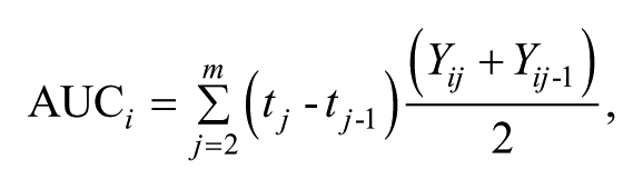
where Y_ij is the observed PRO for the ith subject at the jth time, j = 1, . . ., m, and Y_ij _{− 1} is the j − 1th time for the ith subject. This is simply the area of each trapezoid formed by connecting consecutive Y values and is a weighted linear combination of individual measurements with the average PRO level of each pair of adjacent assessments weighted by the duration of the time period between those two assessments, summed over m − 1 time periods. Because groups can be compared using the difference in mean AUC with a t test (or similar, including linear regression if covariates are to be included), the advantage of this approach is its simplicity. The assumptions are also simple: When the sample size is large enough, AUC and the difference in AUC are approximately normally distributed, even when they are made up of non-normal observations. A clear disadvantage to this approach is that there is no unified principle for handling missing data.

Various ad hoc approaches for handling missing data have been used with summary measures. These include complete case analysis, where patients who drop out are excluded (e.g., Cheng et al., 2010; Ishihara, 1999); last observation carried forward (LOCF; Akhtar-Danesh, 2001) where missing data are replaced with the last observed value; mean imputation (Carusone, Goldsmith, Smieja, & Loeb, 2006) where an individual’s missing data are replaced with the mean of their observed data; extrapolation (Carusone et al., 2006); and interpolation (Qian et al., 2000). The latter four approaches are forms of simple imputation and are prone to inflating the Type I error rate due to variance underestimation and overstatement of the sample size (see Chapter 8 in D. F. Fairclough, 2010).

Summary Statistics for Groups

Summary statistics for computing AUC are obtained post estimation from the parameter estimates of a multivariate model, often a mixed model. For the kth group, the equation is

{\hat{{AUC}_{k}}}_{k} = \sum_{j = 2}^{m} (t_{j} - t_{j - 1}) \frac{({\hat{μ}}_{k j} + {\hat{μ}}_{k j - 1})}{2},

where ${\hat{μ}}_{k j}$ is the kth group’s expected value of Y at time j and is estimated using a linear combination of the parameter estimates after a model has been fit. This could be accomplished by using an estimate statement in SAS, or a lincom statement in Stata, which would also be used to estimate differences in AUC. If there are no missing data, and a saturated mixed model (see below) unadjusted for covariates (beyond time and group assignment) is used, the AUC estimated in this way is the same as the mean of the individual AUCs. With summary statistics, the modeling deals with missing data (see below).

Mixed Models

Mixed models comprise a flexible family of regression models that allows for non-independent data, like in longitudinal studies (Fitzmaurice, Laird, & Ware, 2011). When time is included as a categorical factor, so that the mean at each time is computed, they are sometimes referred to as means models, response profile analyses, saturated models, or repeated-measures mixed models (D. F. Fairclough, 2010; Fitzmaurice et al., 2011; Mallinckrodt, Clark, Carroll, & Molenberghs, 2003). When time is included as a continuous variable, these models have been referred to as linear mixed models or growth curve models. Estimation is performed by maximum likelihood, or more often, restricted maximum likelihood. Observed data lend information about missing data and give mixed models the appealing feature that missing data, as long as it is MCAR or MAR, do not result in biased estimates, if the model is correctly specified (D. F. Fairclough, 2010; Fitzmaurice et al., 2011). If data are MAR, missingness depends on observed data and covariates, so omission of an important covariate or some of the observed data would be an incorrect specification of the model.

PRO Trajectories and Summaries

Summaries have been used to aid in interpretation as well as reducing the number of statistical tests and the subsequent increased likelihood of Type I errors (D. F. Fairclough, 2010). Matthews, Altman, Campbell, and Royston (1990) and D. F. Fairclough (2010) have discussed various outcome trajectories, summaries, and potential hypotheses that may be appropriate for them. For example, if the PRO is changing in a way that is known to be relatively constant over time, the best summary might be the slope. If the treatment effect is transient, and the question of interest is whether there is a difference at a specific time point or whether there is a difference in worst symptoms experienced, then the minimum or maximum might be the most appropriate summary. Sustained effects over time might best be assessed by AUC or the mean over time (these are similar when times between assessments are equal; Curran et al., 2000).

Simulation Study

We address the aims of our study by varying the trajectories, as well as the type and rates of missing data as shown in Table 1. Each of the methods for imputing missing values for the calculation of the summary measures is a common approach in applied research, as described earlier. Sample size, covariance parameters, and baseline values were held constant and informed by QoL data from Study 1.

Table 1.

Simulation Set-Up. 100,000 Samples of Each Combination of Data Pattern, Missingness, and Missingness Allocation Were Simulated.

Data pattern/PRO trajectory^a	Missingness	Missingness allocation between groups	Analysis	Summary measures missing data approaches
1. Linear decline	1. Complete	1. Equal (30% in each group)	1. Mixed model summary statistic	1. Complete case analysis
β = (77, 75, 73, 71, 69, 77, 76.5, 76, 75.5, 75)	2. MCAR	2. Unequal (20% in treatment, 30% in control)	2. Individual summary measures	2. Extrapolation
2. Plateau	3. MAR			3. M imputation
β = (77, 73, 69, 69, 69, 77, 76.5, 76, 75.5, 75)	4. MNAR			4. LOCF
3. Temporary change
β = (77, 70, 76, 76, 76, 77, 76, 75, 75.5, 76)

Note. PRO = Patient reported outcomes; MCAR = missing completely at random; MAR = missing at random; MNAR = missing not at random; LOCF = last observation carried forward.

β refers to the vector of coefficients in Equation 1.

Underlying Model

We simulated data for a randomized, two group, longitudinal design of five time points, using a repeated-measures (means) mixed model:

Y_{i j} = β_{1} t 1 + β_{2} t 2 + β_{3} t 3 + β_{4} t 4 + β_{5} t 5 + β_{6} {group}_{i} \times t 1 + β_{7} {group}_{i} \times t 2 + β_{8} {group}_{i} \times t 3 + β_{9} {group}_{i} \times t 4 + β_{10} {group}_{i} \times t 5 + b_{i} + e_{i j},

where Y_ij is the outcome for the ith subject at the jth time i = 1, . . ., n = 200, j = 1, . . ., m = 5, t1 is an indicator variable for time 1 (t2 for time 2, etc., with subscripts suppressed as common times are used for all subjects), group_i = 0 (control), 1 (treatment), b_i ~ N(0, $σ_{b}^{2}$ ) represents between-person effects, $σ_{b}^{2}$ = between-person variance, e_ij ~ N(0, $σ_{e}^{2}$ ) represents within-person effects, and $σ_{e}^{2}$ = within-person variance. The error terms were independent. Based on the ovarian cancer data, we set the mean baseline (for both groups) to 77, $σ_{b}^{2}$ = 150, $σ_{e}^{2}$ = 60 and within-person correlation over time 0.7. Beta values varied by trajectory, and are given in Table 1.

To mimic ceiling effects commonly found in PRO data, we used a truncated normal distribution. Truncation was achieved by conditioning within the program to re-draw if any Y_ij were less than 0 or greater than 100, conditional on the random effect b_i. This approach resulted in a smooth distribution, rather than creating spikes at 0 or 100, that occurred when a simple substitution rule was used. We simulated 100,000 samples for each of three patterns of change over time, selected to illustrate a range of plausible patterns of QoL in cancer clinical trials (Figure 2), informed by discussion with biostatisticians and researchers in the field.

Figure 2.

Simulated QoL data patterns over time.

Missing Data Patterns

For each of the three data patterns, we simulated data that were complete, MCAR, MAR, and MNAR. The effect of treatment on missingness was considered by using equal drop-out rates between the two groups, at approximately 30%; and unequal dropout rates between groups, with 20% missing in the treatment group and 30% missing in the control group. Missing data were created as follows. For each subject i, and at each time j > 1, the probability that y_ij was set to missing, P(M_ij = 1), was a function of that subject’s previous value, y_ij _{− 1}, to create MAR data. The subject’s current value, y_ij, was conditioned on to create data that were MNAR. Specifically, for MAR, $P (M_{i j} = 1) = 1 / (1 + e^{- θ_{j}})$ , where $θ_{j} = y_{i j - 1} / {\bar{y}}_{j - 1} \log (p_{j} / 1 - p_{j})$ , and ${\bar{y}}_{j - 1}$ = the mean of y at the j − 1th time point. The value p_j varied depending on the trajectory and on whether missingness was allocated equally or unequally, for example, using equal missingness between groups and the linear decline, the vector p = .05, .07, .09, .12. MCAR missing data were created by random deletion. To make the missing data as realistic as possible, we increased the proportion of missingness with each time point. Only monotone (dropout) missing patterns were simulated.

As a sensitivity analysis, a threshold missingness mechanism was also used: for MAR, if y_ij _{− 1} < threshold, then delete y_ij with a given probability; for MNAR, if y_ij < threshold, then delete y_ij with a given probability. Details are given in the appendix.

Calculation of Summary Measures

The summary measure AUC was calculated from the raw data, with each patient’s five PRO measurements summarized into one value. We handled missing data in the following ways: (a) complete case analysis only, (b) linear extrapolation by individual using the previous two observations (requiring at least two observations), (c) imputation using the mean of the individuals’ previously observed data, and (d) LOCF.

Analysis Approaches

In each data set, the difference in AUC between the groups was estimated using a t test for summary measures and a mixed model and contrast for the summary statistic AUC. The t test tested the null hypothesis $H_{0} :_{μ AUC}_{0} = μ_{AUC}_{1}$ , where $μ_{AUC}_{0}$ is estimated by ${\bar{AUC}}_{0} = 1 / n \sum_{i = 1}^{n} {AUC}_{i}$ , for example, for the control group. The mixed model included time as a categorical variable, group, and the interaction of time by group, as well as a random intercept (a means model). Using the model in Equation 1, the estimated mean at any time j = 1, . . ., m = 5 is ${\hat{μ}}_{j} = {\hat{β}}_{j} + {\hat{β}}_{j + m} \times group$ , where group = 0,1; the difference in means between groups is ${\hat{β}}_{j + m}$ ; and the difference in AUC is $\hat{{AUC}_{1}} - \hat{{AUC}_{0}} = 1 / 2 ({\hat{β}}_{6} + 2 {\hat{β}}_{7} + 2 {\hat{β}}_{8} + 2 {\hat{β}}_{9} + {\hat{β}}_{10}) .$

Percent bias for the test of difference between groups was computed by 100 × (estimate − true value) / true value, so that positive values indicate overestimates and negative values represent underestimates. We also present the bias divided by the estimated standard error (SE) that represents how far off the t statistic for the test of difference in AUC is from the t statistic computed from a non-biased estimate. A small value, say less than 0.1, is unlikely to change conclusions. Precision of estimates of difference in AUC are given by the width of the 95% confidence interval (CI) width. All simulations and analyses were performed in SAS v9.2.

Simulation Results

Missingness rates for the simulated data are shown in Table 2, for the MAR case. Rates at each time point for the MCAR and MNAR data were similar and are not shown. The difference in AUC between groups was normally distributed, despite having come from a truncated normal distribution. This is to be expected based on the central limit theorem but is mentioned to underscore the validity of parametric approaches.

Table 2.

Percentage of MAR^a Missing Data at Each Time Point by Data Pattern and Group.

			Time
Allocation of missingness	Data pattern	% missing	1	2	3	4	5
Equal	Linear decline	Control	0	6	13	21	31
	Linear decline	Treatment	0	6	13	21	30
	Plateau	Control	0	5	13	22	31
	Plateau	Treatment	0	5	12	20	28
	Temporary change	Control	0	5	13	21	30
	Temporary change	Treatment	0	5	12	20	29
Unequal	Linear decline	Control	0	6	13	22	31
	Linear decline	Treatment	0	4	9	14	20
	Plateau	Control	0	5	12	21	31
	Plateau	Treatment	0	4	9	14	20
	Temporary change	Control	0	5	13	21	29
	Temporary change	Treatment	0	4	8	14	20

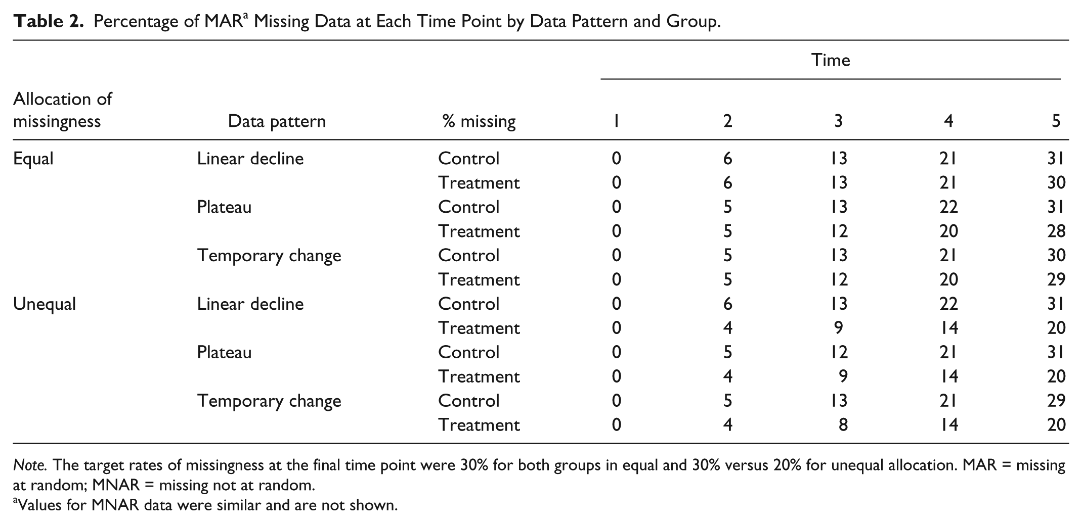
Note. The target rates of missingness at the final time point were 30% for both groups in equal and 30% versus 20% for unequal allocation. MAR = missing at random; MNAR = missing not at random.

Values for MNAR data were similar and are not shown.

The main results from the simulations are shown in Table 3. When no data were missing, there was no bias for the AUC estimated from the parameters of a mixed model (summary statistic) or the AUC computed from individual summary measures.

Table 3.

Comparison of Individual Summary Measures With Mixed Model Summary Statistics: Estimated Difference in AUC (Treat − Control), Percent Bias, and Precision^a for 100,000 Samples of n = 200 Subjects.

		Equal missingness				Unequal missingness
Data pattern and missingness	AUC approach and imputation method	95% CI width	Estimate	Percent bias	Bias/SE	Estimate	Percent bias	Bias/SE
Linear decline
No missing data	Individual AUC	26.3	11.14	0	0	11.14	0	0
	Mixed model AUC	26.3	11.14	0	0	11.14	0	0
MCAR	Individual AUC
	1. Complete case^b	31.6	11.15	0.1	0	11.15	0.1	0
	2. Extrapolation	29.3	11.12	−0.2	0	11.10	−0.3	0
	3. M imputation	26.7	9.44	−15.2	−0.25	9.21	−17.4	−0.28
	4. LOCF	27.3	8.64	−22.4	−0.36	8.48	−23.9	−0.38
	Mixed model AUC	26.7	11.14	0	−0.01	11.14	0	0
MAR	Individual AUC
	1. Complete case^b	30.5	10.53	−5.6	−0.08	9.37	−15.8	−0.24
	2. Extrapolation	29.8	11.20	0.5	0.01	11.28	1.4	0.02
	3. M imputation	26.6	9.27	−16.8	−0.28	9.18	−17.5	−0.29
	4. LOCF	27.4	8.52	−23.6	−0.38	8.51	−23.5	−0.38
	Mixed model AUC	26.7	10.8	−0.6	−0.01	11.05	−0.7	−0.01
MNAR	Individual AUC
	1. Complete case	30.4	10.23	−8.3	−0.11	9.08	−18.4	−0.27
	2. Extrapolation	29.3	10.97	−1.6	−0.02	10.62	−4.5	−0.07
	3. M imputation	26.4	9.12	−18.1	−0.30	8.82	−20.7	−0.34
	4. LOCF	27.1	8.41	−24.6	−0.40	8.16	−26.7	−0.43
	Mixed model AUC	26.5	10.96	−1.7	−0.03	10.73	−3.6	−0.06
Plateau
No missing data	Individual AUC	26.5	18.66	0	0	18.66	0	0
	Mixed model AUC	26.5	18.66	0	0	18.66	0	0
MCAR	Individual AUC
	1. Complete case^b	31.9	18.65	0	0	18.65	0	0
	2. Extrapolation	29.6	19.85	0	0.16	19.85	6.4	0.16
	3. M imputation	26.9	16.53	−11.4	−0.31	16.30	−12.7	0.34
	4. LOCF	27.6	17.71	−5.1	−0.13	17.56	−5.9	−0.15
	Mixed model AUC	26.5	18.66	0	0	18.66	0	0
MAR	Individual AUC
	1. Complete case	30.5	17.50	−6.2	−0.15	16.58	−11.3	−0.28
	2. Extrapolation	30.2	20.25	8.5	0.21	20.48	9.5	0.23
	3. M imputation	26.7	16.31	−12.6	−0.34	16.35	−12.5	−0.34
	4. LOCF	27.5	17.62	−5.6	−0.15	17.75	−8.1	−0.13
	Mixed model AUC	26.8	18.58	−0.4	−0.01	18.61	−0.5	−0.01
MNAR	Individual AUC
	1. Complete case	30.7	17.23	−7.7	−0.18	16.27	−13.0	−0.32
	2. Extrapolation	29.7	19.74	5.8	0.14	19.60	4.9	0.12
	3. M imputation	26.5	15.91	−14.7	−0.40	15.83	−15.0	−0.42
	4. LOCF	27.3	17.21	−7.8	−0.21	17.18	−5.1	−0.22
	Mixed model AUC	26.6	18.36	−1.6	−0.04	18.23	−0.7	−0.07
Temporary change
No missing data	Individual AUC	26.2	4.23	0	0	4.25	0	0
	Mixed model AUC	26.1	4.23	0	0	4.25	0	0
MCAR	Individual AUC	26.1	4.23	0	0
	1. Complete case^b	31.4	4.26	0.6	0	4.26	0.2	0
	2. Extrapolation	29.7	5.76	36.1	0.2	5.97	40.5	0.2
	3. M imputation	26.6	4.87	15.2	0.01	4.67	10.0	0.06
	4. LOCF	27.3	4.58	7.5	0.05	4.39	3.3	0.02
	Mixed model AUC	26.5	4.23	0	0	4.25	0	0
MAR	Individual AUC
	1. Complete case	30.0	3.94	−6.8	−0.04	3.00	−29.3	−0.17
	2. Extrapolation	30.8	6.73	59.0	0.31	7.10	66.9	0.36
	3. M imputation	26.7	4.96	17.3	0.11	4.97	16.8	0.11
	4. LOCF	27.6	4.82	14.0	0.08	4.92	15.7	0.10
	Mixed model AUC	26.5	4.25	0.5	0	4.27	0.3	0.002
MNAR	Individual AUC
	1. Complete case	30.0	3.97	−6.1	−0.03	3.02	−29.0	−0.17
	2. Extrapolation	29.8	5.81	37.4	0.20	5.55	30.5	0.17
	3. M imputation	26.4	4.74	12.1	0.08	4.60	8.2	0.05
	4. LOCF	27.2	4.50	6.3	0.04	4.35	2.2	0.01
	Mixed model AUC	30.0	3.94	−6.8	−0.04	3.00	−29.3	−0.17

Note. Results for precision were similar for the case of equal and unequal missing data rates in the two groups so only equal rates’ results are shown. AUC = area under the curve; CI = confidence interval; SE = standard error; MCAR = missing completely at random; LOCF = last observation carried forward; MAR = missing at random; MNAR = missing not at random.

Percent bias is 100 × (estimate − true) / true. Width of 95% CI reflects precision.

Only patients with complete data were analyzed.

Negative values indicate underestimation of the difference in AUC between groups.

The mixed model estimates showed negligible bias for both MCAR and MAR data: less than 1% for all patterns and drop-out rates. When the data were MNAR, the bias of the mixed model estimates was low for most scenarios, except for the temporary change, unequal drop-out case, which had a 29% underestimation.

Bias for all the individual AUC approaches (complete case and simple imputation) was larger, ranging from 27% underestimation to 67% overestimation, and varied according to the imputation method and data pattern. Complete case analyses yielded unbiased results for MCAR data, as expected. For MAR and MNAR data, the bias ranged from −29% to −6%. Simple imputation methods yielded bias for all scenarios, even in the MCAR case. For example, bias with LOCF ranged from −24% to 8% for MCAR data, and −24% to 16% for the MAR case.

Precision, as measured by the 95% CI widths was comparable for all patterns, although the mixed models had slightly smaller CI widths and the complete case analysis consistently had the largest CI widths, due to smaller sample size. The results using the threshold drop-out mechanism (the sensitivity analysis) showed very similar patterns (see the appendix).

Renal Carcinoma Example

Summary measures using the various simple imputation techniques and summary statistics computed from a mixed model as described above were computed. The results are shown in Figure 3 and Table 4. The most dramatic and not unexpected result occurs with the complete case analysis, with an estimated treatment difference of 0.56 as compared with the mixed model estimate of −20.8. This illustrates the impact of selection bias; when analysis is limited to those patients who stay on trial (most of whom remained progression free) and assume that missingness is completely unrelated to the outcome, we see no differences across treatment. In contrast, when we implement methods that attempt to address missing data, we identify a difference between the treatment arms. The simple imputation methods all gave similar results (about −16, favoring the control arm). Assuming that the data are MAR and the model was specified correctly so that the mixed model estimate is correct, the estimated bias is about 24%.

Figure 3.

Quality of lifetime trajectories, by treatment group and analytical approach.

Table 4.

Estimates of Difference in QoL AUC (Treat − Control) for Renal Carcinoma RCT Data.

Approach	Analysis	Estimate	95% CI	p value
Summary Statistics	Mixed model	−20.8	[−33.6, −7.9]	.002
Summary Measures	Complete case	0.56	[−17.5, 18.7]	.95
	Extrapolation	−16.3	[−31.8, −0.80]	.04
	M imputation	−15.7	[−26.7, −4.8]	.005
	LOCF	−16.8	[−28.3, −5.3]	.005

Note. QoL = quality of life; AUC = area under the curve; RCT = randomized controlled trial; CI = confidence interval; LOCF = last observation carried forward.

With regard to PRO trajectories over time, we note that the extrapolation technique appears to stand out in contrast to the other methods (Figure 2). This does not imply that this technique is consistently problematic but clearly illustrates that imputation choices are very trial specific and difficult to make a priori.

Discussion

We conducted a simulation study to compare the performance of the AUC computed in two ways, as a raw data summary measure where each individual’s PRO over time reduces to one number that can then be compared between groups with a t test; and using summary statistics, in which AUC is computed for groups based on estimated parameters from a mixed model. We aimed to examine the bias of these two methods and their sensitivity to assumptions about missing data and patterns of change. With no missing data, the two approaches gave identical results. With any type of missing data, summary statistics were consistently superior to summary measures, in terms of bias and precision. The bias resulting from the summary statistic approach was very small, even when data were MNAR. The bias resulting from the summary measure approach was considerable under some conditions, and importantly, the size and direction of bias was unpredictable, varying with data pattern, missingness, and imputation method. The complete case analysis of AUC summary measures consistently had the lowest precision (due to reduced sample size), and the bias with this approach doubled when the rate of missing data differed between groups. These results were consistent when group missing data rates were equal and unequal.

Relation to Other Literature

Various statisticians (Carpenter & Kenward, 2008; D. F. Fairclough, 2010; Mallinckrodt et al., 2003; Molenberghs et al., 2004) have warned about the bias that can occur with LOCF. Despite these warnings, LOCF is still often used (Fielding et al., 2008; Wood et al., 2004). We found that LOCF underestimated the treatment effect by approximately 25% in the linear decline pattern even when data were MCAR or MAR. In contrast, for the temporary decline pattern, it produced overestimates. This illustrates the findings of Molenberghs et al. (2004, p.454) who demonstrated algebraically that even when data are MCAR, “the bias can be positive or negative and can even induce an apparent treatment effect when one does not exist.”

Our results confirm Bell, Kenward, Fairclough, and Horton (2013) by demonstrating that equal dropout between groups does not imply unbiased results; we have shown that even if the missingness patterns are similar between the groups, the use of individual summary measures can cause considerable bias.

Although summary measures are equivalent to summary statistics (for certain models, such as those shown here), when no data are missing, a complete data set in longitudinal studies is rare, so missingness must be considered in any valid analysis. Qian et al. (2000, p.2672) stated that they assumed the data were MCAR because the patterns of missingness between the treatment groups were similar and also because “they wanted to keep the analyses manageable and it is not easy to identify the missing value processes in practice.” Simplicity is an admirable goal, but it should not be used to the detriment of the validity of the study. Perhaps researchers use simple imputation methods because of a desire to follow the intention to treat principle and are not aware that likelihood methods can be consistent with this principle (Molenberghs et al., 2004).

When maximum likelihood was used, there was minimal bias in the MNAR scenarios. This finding is consistent with others (Mallinckrodt et al., 2003; Molenberghs et al., 2004), but generalizations should be formed cautiously, as different drop-out mechanisms may show a larger influence.

Recommendations

Although maximum likelihood methods including mixed models are not simple, there are types that are simpler than others, such as the means model with a random intercept in the RCT setting, as shown in this article, or the so-called mixed effects repeated-measures model (Mallinckrodt et al., 2003). Both of these models, because they use time categorically, are robust to misspecification of the outcome’s mean structure over time. While some have argued that the compound symmetric correlation structure assumed by this model is unrealistically simple (Fitzmaurice et al., 2011), others have argued that this is a reasonable assumption in the context of RCTs (Frison & Pocock, 1992). The correlation over time in the PRO data from both examples was well approximated with a compound symmetric structure. There are trade-offs between complexity and simplicity, but we believe that the advantage of having the potential of no bias for data that are MAR, and possibly reduced bias for MNAR in a range of scenarios, outweighs the benefits of the simplicity of summary measures. Leaders in the missing data field have recommended that the MAR assumption is the best starting point for analyses (7, 23, 24, 26, 27), and we recommend it for summaries also.

Limitations

There are limitations to our research. We examined a limited number of missing data scenarios. There are different types of missingness mechanisms, that is, methods of creating missing data that may influence results to a degree; we examined two among many possible probabilistic models for dropout as a function of the outcome. The data were generated using a mixed model, similar to the one used to model the data and may contribute to the low level of bias using mixed models. We only considered one covariance structure (compound symmetry), explored a limited number of trajectories, and considered only dropout. However, in our experience, dropout is a larger problem than intermittent missing data. Multiple imputation was not explored. However, if multiple imputation is used but without auxiliary data, results will be nearly identical to those from a mixed model fitted to the incomplete data set (D. F. Fairclough, 2010).

Conclusion

If AUC is used as a longitudinal summary when data are not MCAR, it should be estimated using maximum likelihood (such as a mixed model) using summary statistics rather than from individuals’ summary measures to minimize bias in treatment effect estimation. An area of future research is how the results presented here could be applied in the field pharmacokinetic analyses.

Footnotes

Appendix

To ascertain whether the results were influenced by the methods of creating missing data, we performed a sensitivity analysis using 1,000 samples with a different method.

MAR data were created as follows. Let M_ijk = 1 if the outcome Y_ijk is missing for the ith subject at the jth time in the kth group (k = 0,1). Then

P (M_{i j k} = 1) = c \times [1 - Φ (Y_{i (j - 1) k}, {\bar{Y}}_{(j - 1) k}, σ)],

where

c = 0.18 and Φ is the value of the cumulative distribution function at Y_i_{(j − 1)k} for a normal distribution with mean ${\bar{Y}}_{k (j - 1)}$ (the mean for the kth group at the time point previous to the jth) and standard deviation σ. For MNAR data, the current value, Y_ijk and ${\bar{Y}}_{j k}$ were used.

The results given in Table A1 are nearly identical to the original results in the article.

Declaration of Conflicting Interests

The author(s) declared no potential conflicts of interest with respect to the research, authorship, and/or publication of this article.

Funding

The author(s) disclosed receipt of the following financial support for the research and/or authorship of this article: Data presented are derived (and used with permission) from a trial conducted by Memorial Sloan-Kettering Cancer Center and Eastern Cooperative Oncology Group funded by the National Cancer Institute Grant CA-05826.

Author Biographies

Melanie Bell is Associate Professor of Biostatistics at the Mel & Enid Zuckerman College of Public Health at the University of Arizona. She is involved in clinical trials research, particularly with regard to missing data and patient reported outcomes.

Professor Madeleine King is the first Cancer Australia Chair in Cancer Quality of Life. She is involved in building collaborative research efforts in quality of life research in the Australian cancer community.

Professor Diane Fairclough is a past President of the International Society for Quality of Life Research and is the author of Design and Analysis of Quality of Life Studies in Clinical Trials, 2nd edition (2010). Dr. Fairclough’s primary research interest is Quality of Life, outcomes in palliative/hospice care, and psychosocial sequelae of cancer and its therapy in pediatric and adult patients.

References

Akhtar-Danesh

(2001). A review of statistical methods for analysing pain measurements. European Journal of Pain, 5, 457-463.

Bell

M. L.

Fairclough

D. L.

(2013). Practical and statistical issues in missing data for longitudinal patient reported outcomes. Statistical Methods in Medical Research. Advance online publication. doi:10.1177/0962280213476378 Retrieved from http://smm.sagepub.com/content/early/2013/02/14/0962280213476378.long

Bell

M. L.

Kenward

H. G.

Fairclough

D. L.

Horton

N. J.

(2013). Differential dropout and bias in randomised controlled trials: When it matters and when it may not. British Medical Journal, 346, e8668.

Carpenter

Kenward

(2008). Missing data in randomised controlled trials—A practical guide (Vol. Publication RM03/JH17/MK). Retrieved from http://www.pcpoh.bham.ac.uk/publichealth/methodology/projects/RM03_JH17_MK.shtml

Carusone

S. C.

Goldsmith

C. H.

Smieja

Loeb

(2006). Summary measures were a useful alternative for analyzing therapeutic clinical trial data. Journal of Clinical Epidemiology, 59, 387-392.

Cella

D. F.

Tulsky

D. S.

Gray

Sarafian

Linn

Bonomi

. . .Bonomi

(1993). The functional assessment of cancer therapy scale: Development and validation of the general measure. Journal of Clinical Oncology, 11, 570-579.

Cheng

K. K.

Leung

S. F.

Liang

R. H.

Tai

J. W.

Yeung

R. M.

Thompson

D. R.

(2010). Severe oral mucositis associated with cancer therapy: Impact on oral functional status and quality of life. Supportive Care in Cancer, 18, 1477-1485.

Cox

D. R.

Fitzpatrick

Fletcher

A. E.

Gore

S. M.

Spiegelhalter

D. J.

Jones

D. R.

(1992). Quality-of-life assessment: Can we keep it simple? Journal of the Royal Statistical Society: Series A, Statistics in Society, 155, 353-393.

Curran

Aaronson

Standaert

Molenberghs

Therasse

Ramirez

. . .Piccart

(2000). Summary measures and statistics in the analysis of quality of life data: An example from an EORTC-NCIC-SAKK locally advanced breast cancer study. European Journal of Cancer, 36, 834-844.

10.

Dawson

J. D.

(1994). Stratification of summary statistic tests according to missing data patterns. Statistics in Medicine, 13, 1853-1863.

11.

Fairclough

D. F.

(2010). Design and analysis of quality of life studies in clinical trials (2nd ed.). Boca Raton, FL: Chapman & Hall/CRC.

12.

Fairclough

D. L.

(1997). Summary measures and statistics for comparison of quality of life in a clinical trial of cancer therapy. Statistics in Medicine, 16, 1197-1209.

13.

Fielding

Maclennan

Cook

J. A.

Ramsay

C. R.

(2008). A review of RCTs in four medical journals to assess the use of imputation to overcome missing data in quality of life outcomes. Trials, 9, Article 51.

14.

Fitzmaurice

G. M.

Laird

N. M.

Ware

J. H.

(2011). Applied longitudinal analysis (2nd ed.). Hoboken, NJ: John Wiley.

15.

Food and Drug Administration. (2009). Guidance for industry on patient-reported outcome measures: Use in medical product development to support labeling claims (Vol. 74. pp. 65132-65133): Federal Register, Washington, DC.

16.

Frison

Pocock

S. J.

(1992). Repeated measures in clinical trials: Analysis using mean summary statistics and its implications for design. Statistics in Medicine, 11, 1685-1704.

17.

Ishihara

(1999). A diary form quality of life questionnaire for Japanese patients with lung cancer and summarization techniques for longitudinal assessment. Respirology, 4, 53-61.

18.

Little

R. J.

Raghunathan

(1999). On summary measures analysis of the linear mixed effects model for repeated measures when data are not missing completely at random. Statistics in Medicine, 18, 2465-2478.

19.

Little

R. J. A.

Rubin

D. B.

(1987). Statistical analysis with missing data. New York, NY: John Wiley.

20.

Mallinckrodt

C. H.

Clark

W. S.

Carroll

R. J.

Molenberghs

(2003). Assessing response profiles from incomplete longitudinal clinical trial data under regulatory considerations. Journal of Biopharmaceutical Statistics, 13, 179-190.

21.

Matthews

J. N. S.

Altman

D. G.

Campbell

M. J.

Royston

(1990). Analysis of serial measurements in medical research. British Medical Journal, 300, 230-235.

22.

Molenberghs

Thijs

Jansen

Beunckens

Kenward

M. G.

Mallinckrodt

Carroll

R. J.

(2004). Analyzing incomplete longitudinal clinical trial data. Biostatistics, 5, 445-464.

23.

Neoptolemos

J. P.

Stocken

D. D.

Friess

Bassi

Dunn

J. A.

Hickey

. . .Büchler

M. W.

(2004). A randomized trial of chemoradiotherapy and chemotherapy after resection of pancreatic cancer. New England Journal of Medicine, 350, 1200-1210. doi:10.1056/NEJMoa032295

24.

Patrick

D. L.

Burke

L. B.

Powers

J. H.

Scott

J. A.

Rock

E. P.

Dawisha

. . .Kennedy

D. L.

(2007). Patient-reported outcomes to support medical product labeling claims: FDA perspective. Value in Health, 10(Suppl. 2), S125-S137.

25.

Price

Bell

Sommeijer

Friedlander

Stockler

Defazio

. . .Butow

(2013). Physical symptoms, coping styles, and quality of life in recurrent ovarian cancer: A prospective population-based study over the last year of life. Gynecologic oncology, 130, 162-168.

26.

Qian

Parmar

M. K. B.

Sambrook

R. J.

Fayers

P. M.

Girling

D. J.

Stephens

R. J.

(2000). Analysis of messy longitudinal data from a randomized clinical trial. Statistics in Medicine, 19, 2657-2674.

27.

Vasey

P. A.

Jayson

G. C.

Gordon

Gabra

Coleman

Atkinson

, . . . On the Behalf of the Scottish Gynaecological Cancer Trials Group. (2004). Phase III randomized trial of docetaxel–carboplatin versus paclitaxel–carboplatin as first-line chemotherapy for ovarian carcinoma. Journal of the National Cancer Institute, 96, 1682-1691. doi:10.1093/jnci/djh323

28.

Wood

A. M.

White

I. R.

Thompson

S. G.

(2004). Are missing outcome data adequately handled? A review of published randomized controlled trials in major medical journals. Clinical Trials, 1, 368-376.

Bias in Area Under the Curve for Longitudinal Clinical Trials With Missing Patient Reported Outcome Data

Abstract

Keywords

Introduction

Missing Data

Summary Measures and Statistics

Literature

Aim

Motivating Examples

AUC: Summary Measures and Summary Statistics

Summary Measures for an Individual

Summary Statistics for Groups

Mixed Models

PRO Trajectories and Summaries

Simulation Study

Underlying Model

Missing Data Patterns

Calculation of Summary Measures

Analysis Approaches

Simulation Results

Renal Carcinoma Example

Discussion

Relation to Other Literature

Recommendations

Limitations

Conclusion

Footnotes

Appendix

Declaration of Conflicting Interests

Funding

Author Biographies

References