The development of the classical Chinese algebra of polynomials: From the Nine Chapters and Liu Hui through Wang Xiaotong,Li Ye and Zhu Shijie

Abstract

The remarkable algebra of polynomials used by mathematicians in the Song and Yuan periods was the product of a development that started in the Han period or before. This article traces that development through examples from four important books.

1. Introduction

Mathematical texts from the Song and Yuan periods use a remarkably sophisticated algebraic method, describing manipulations of what we would call ‘polynomial expressions’ to solve geometric problems. This was the highest point of a development that started more than a millennium before, with the Nine Chapters on the Art of Mathematics (Jiuzhang suanshu 九章算术, hereafter the Nine Chapters) ¹ and Liu Hui (刘徽; 3rd century CE). In this article, I analyse examples from four mathematical books and show some high points in the development of the system.

The story starts with Liu Hui's geometric explanation of the square- and cube-root algorithms in the Nine Chapters. These are essentially methods of numerical solution of the simple polynomial equations $x^2=a$ and $x^3=a$ . One geometric problem in the book involves what amounts to the solution of a non-trivial quadratic equation, $x^2+34x=71,000$ . Wang Xiaotong in the 7th century used ad hoc geometric constructions to create cubic equations that can be solved numerically. Li Ye in the thirteenth century manipulated polynomial expressions without reference to their geometric origin. Zhu Shijie in 1303 extended the system in a number of ways, the most important of which is that he dealt with polynomials of more than one variable. After this, the system was completely forgotten until it was revived as a matter of historical interest by mathematicians in the nineteenth century.

2. Liu Hui and the Nine Chapters

The Nine Chapters is certainly the most important book in the history of Chinese mathematics. Its date has long been uncertain. Zou Dahai (2022: 34–51) has reviewed many attempts to date the book and concluded that its origin was before the Qin period, but that it reached its present form in the Western Han period. ² I feel no need to go much further into this question here: the book is early. Liu Hui's commentary, which can be securely dated to 263 CE, corrects, extends and explains its methods. ³

The algorithms for extracting square and cube roots are in Chapter 4 (See Qian, 1963: 149–151; Chemla and Guo, 2004: 322ff., 360–368, 800–804 n. 27–55); Guo et al., 2013: 373–409; Shen et al., 1999: 175ff., 203–213). ⁴ In explaining the square-root algorithm, Liu Hui uses a diagram, now lost, that may have resembled Figure 1d.

Figure 1.

The geometric interpretation of the square-root algorithm in the Nine chapters. a: The given number; b: after determining the first digit of the square root, 2; c: after the second digit, 3; d: after the third and last digit, 5. The result is 235 paces.

Problem 12 in Chapter 4 asks for the square root of 55,225. The Nine Chapters text describes the root extraction step by step, and from its terminology it is clear that this algorithm had from the beginning been interpreted geometrically. Liu Hui makes the geometric interpretation explicit.

See Figure 1 a–d. The starting situation is a square with area 55,225 square paces. The first digit of the root, 2, is determined. Its value is 200 paces; a corresponding square is cut out of the original square, leaving a gnomon with area 15,225 square paces. The second digit is 3, and a gnomon corresponding to 30 paces is removed, leaving 2,325 square paces. The third digit is 5, and when the corresponding gnomon is removed, there is nothing left of the original square. The result is therefore exactly 235 paces.

The Nine Chapters includes in a single case the direct use of the geometric interpretation of the square-root algorithm to solve a geometric problem, Problem 20 in Chapter 9 (see Qian, 1963: 255–256; Chemla and Guo, 2004: 689–693, 736–738; 892–893 n. 107–112; Guo et al., 2013: 1137–1143; Shen et al., 1999: 507–512). This and Liu Hui's comment are translated in Appendix 1.

It is quite possible that Liu Hui provided a diagram, now lost, with his comment, but Figure 2 is simply my diagram, not an attempt to reconstruct his. A square city, LKPS, has gates at B and C, the centres of LK and SP. A tree is at A. Someone walks from C to D and then to E, where he sees the tree. The given quantities are

a = 20 paces

b = 14 paces

c = 1,775 paces

and x is to be calculated. Liu Hui uses the similarity of triangles ABL and ADE to show that 2ac is equal to the area of the rectangle FGHJ. He then dissects and rearranges areas to construct the gnomon LWQPRU in Figure 3, which has the same area and is essentially the same as a result of the first step of the square-root algorithm (Figure 1(b)). Here, ½(a + b) corresponds to the first digit of a square root. Continuing the steps of the algorithm gives x = 250 paces. In a modern interpretation, this corresponds to solving the polynomial

$$x^2+(a+b)x=2ac$$

$$x^2+34x=71,000\mathrm{square}\mathrm{paces}$$

Figure 2.

To illustrate Problem 20 of Chapter 9 in the Nine Chapters.

Figure 3.

The result of dissecting and rearranging parts of Figure 2.

This is then the first known use of a non-trivial polynomial in classical Chinese mathematics, the beginning of a long development. It is interpreted entirely geometrically, without the use of any algebraic reasoning.

3. Wang Xiaotong's Continuation

Wang Xiaotong (王孝通) was an official of the Sui and Tang dynasties concerned with mathematics education, astronomy and the calendar. His dates are tentatively given as ‘579?–638?’. His book, Jigu suanjing (缉古算经, The Continuation of Ancient Mathematics, hereafter the Continuation), was presented to the Tang Emperor around 638 (Lim and Wagner, 2017: 3–5).

In this book, the numerical solution of cubic polynomials by the Chinese version of Horner's method (see Wagner, 2017) is part of the background knowledge assumed on the part of the reader. This root extraction is directly related to the extraction of square and cube roots in the Nine chapters (and other early books), as is clear from the terminology used.

Reading the book, it becomes clear that Wang Xiaotong sees the columns of numbers used in the root-extraction algorithm as representing what we would call equations: they are statements that certain operations on an unknown quantity result in a certain quantity.

3.1 Building a tamped-earth dyke

Two of the problems in Wang Xiaotong's book are translated in appendices 2 and 3. In the first, the second part of Problem 3, the dimensions and volume are given for a tamped-earth dyke (Figure 4) to be built by workers from four counties. The volume that each county is responsible for is given, and the dimensions of the county's part are to be calculated. Many of the book's problems are ‘textbook exercises’ without direct practical application, ⁵ but this one is real, a simplified version of one of the tasks of imperial officials: administering the assignment of corvée labour for public works (Wagner, 2013; Lim and Wagner, 2017: 6–12).

Figure 4.

To illustrate the second part of Problem 3 of Wang Xiaotong's Continuation.

See Figure 4. The dimensions of the whole dyke have been determined in the first part of Problem 3:

a = 80 cun 寸

b₁ = 142 cun

b₂ = 762 cun

h₁ = 31 cun

h₂ = 341 cun

l = 4800 cun

The volume of County A's section is

• V_A = 33,351,040 cun³

In the second part of the problem, the length of County A's section, x, is determined, after which its other dimensions are determined by considering similar triangles. A cubic equation is built up using the volume dissection shown in Figure 5. The volumes of the four parts are all products of known quantities and powers of x:

$$V_{\mathrm{I}}={\displaystyle \frac{1}{2}(a+b_1)h_{1}x=3,441x}$$

$$\begin{array}{r}{V}_{\mathrm{II}}={\displaystyle \frac{1}{2}{\displaystyle \frac{x}{l}(h_2-h_1)b_{1}x={\displaystyle \frac{b_1(h_2-h_1)}{2l}{x}^2={\displaystyle \frac{2,201}{480}{x}^2}}}}\end{array}$$

$$V_{\mathrm{III}}=2\times {\displaystyle \frac{1}{6}{\displaystyle \frac{x}{l}\left({\displaystyle \frac{b_2-b_1}{2}}\right){\displaystyle \frac{x}{l}(h_2-h_1)x={\displaystyle \frac{(b_2-b_1)(h_2-h_1)}{6l^2}{x}^3={\displaystyle \frac{961}{691,200}{x}^3}}}}}$$

$$V_{\mathrm{III}}+V_{\mathrm{II}}+V_{\mathrm{I}}=V_{\mathrm{A}}$$

$$\begin{array}{rl}& {\displaystyle \frac{(b_2-b_1)(h_2-h_1)}{6l^2}{x}^3+{\displaystyle \frac{b_1(h_2-h_1)}{2l}{x}^2}}\\ & +{\displaystyle \frac{1}{2}(a+b_1)h_{1}x=V_{\mathrm{A}}}\end{array}$$

$${\displaystyle \frac{961}{691,200}{x}^3+{\displaystyle \frac{2,201}{480}{x}^2+3,441x=33,351,040cu{n}^3}}$$

Figure 5.

Dissection of Figure 4 to derive the contribution of County A.

However, Wang Xiaotong's cubics always have the cubic coefficient equal to 1. His calculation is therefore

$$x^3+{\displaystyle \frac{3b_{1}l}{b_2-b_1}{x}^2+{\displaystyle \frac{3(b_2-b_1)(h_2-h_1)}{(a+b_1)h_1}{l}^{2}x={\displaystyle \frac{6l^2}{(b_2-b_1)(h_2-h_1)}{V}_{\mathrm{A}}}}}$$

$$x^3+3,298{\displaystyle \frac{2}{31}{x}^2+2,474,941{\displaystyle \frac{29}{31}x=23,987,761,548{\displaystyle \frac{12}{31}cu{n}^3}}}$$

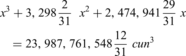
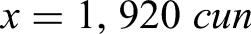
This equation has one real root,

$$x=1,920cun$$

3.2 A triangle problem

At the end of Wang Xiaotong's book are six problems in plane geometry, which he solves using three-dimensional constructions. Two of these, Problems 19–20, are translated in Appendix 3. A challenge here is that all extant versions of the Continuation go back to a damaged copy (now lost) in which large parts of the last pages are fragmentary. Various attempts have been made to reconstruct the original text. These are discussed by Lim and Wagner (2017: 104–108); for convenience, I accept here Zhang Dunren's (张敦仁) reconstruction. Others differ in detail but not in the overall method, which is my concern here.

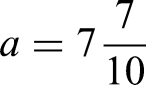
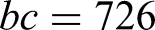
Problem 19 states that in a right triangle (see Figure 6),

$$a=7{\displaystyle \frac{7}{10}}$$

$$bc=726$$

and b is to be determined. No units are given for these quantities. Wang Xiaotong's six triangle problems may be the only place in the entire classical Chinese mathematical corpus in which geometric quantities are stated without units.

Figure 6.

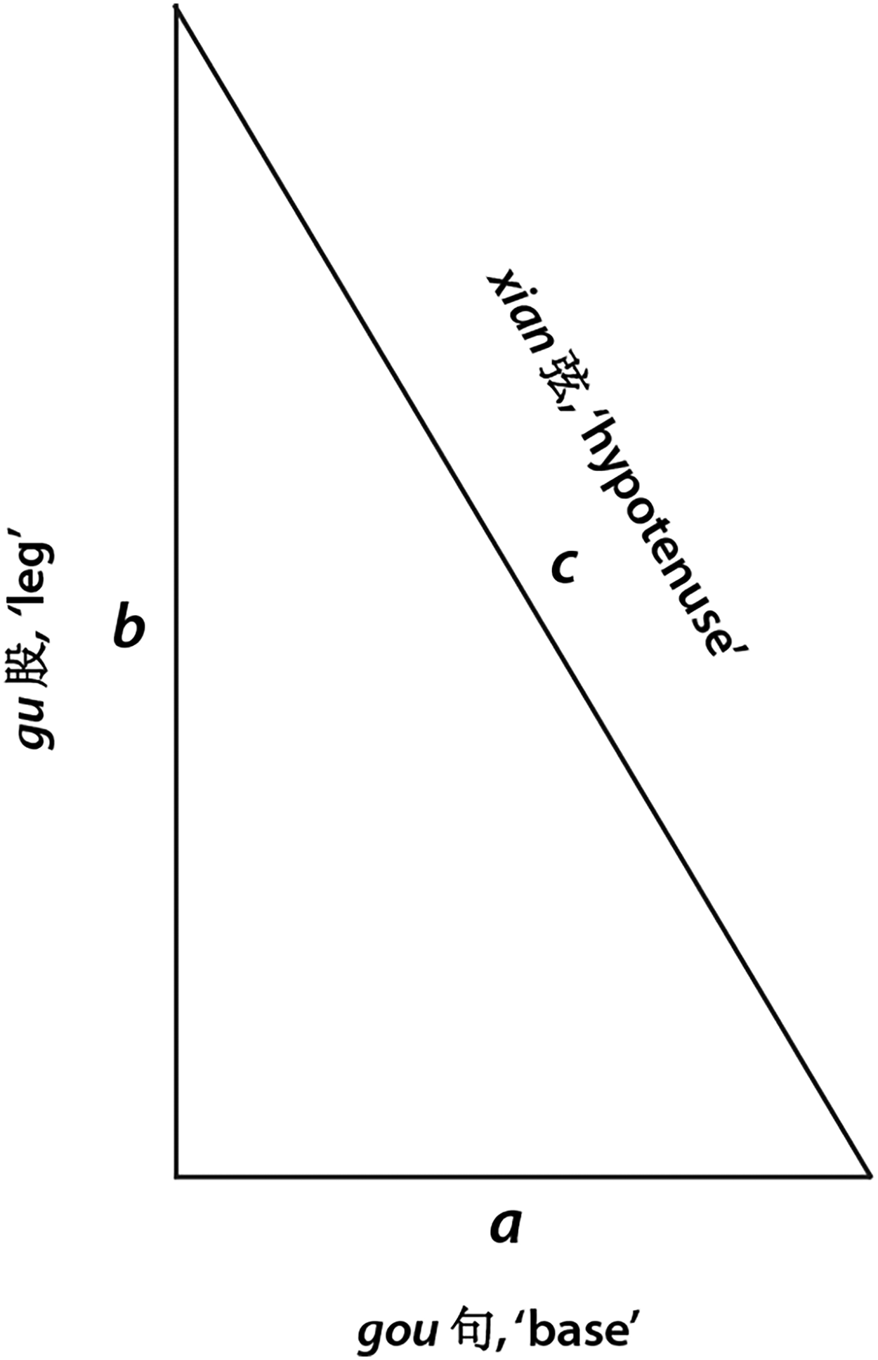
A right triangle, with the classical Chinese names for its parts and their commonest English translations.

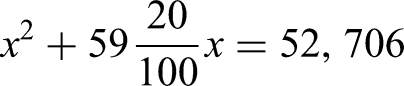
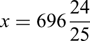
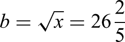
The calculation is then the numerical solution of

$$x^2+a^{2}x=(bc{)}^2$$

(1)

$$x^2+59{\displaystyle \frac{20}{100}x=52,706}$$

in which $x=b^2$ . This has one positive root,

$$x=696{\displaystyle \frac{24}{25}}$$

and

$$b=\sqrt{x}=26{\displaystyle \frac{2}{5}}$$

It is easy to derive (1) algebraically, for

$$b^4+a^2{b}^2=b^2(a^2+b^2)=b^2{c}^2=(bc{)}^2$$

However, what remains of the fragmentary text of a comment in smaller characters appears to imply a geometric explanation. That in turn would seem to imply a four-dimensional construction. But the lack of units in the given quantities makes the construction shown in Figure 7 plausible. Here, both b and b² are used as linear measures. The volume of the solid is $b^2{c}^2$ , and the sum of the two blocks into which the solid is divided is

$$b^4+(c^2-b^2)b^2=x^2+a^{2}x=(bc{)}^2$$

Figure 7.

Proposed construction to derive the leg of a right triangle in Problem 19 of Wang Xiaotong’s Continuation.

These two examples show that an important insight had been gained by Wang Xiaotong's time: the columns of numbers used in root extraction represent what we call polynomial equations, and they can be used in more complex calculations than were dealt with in the Nine Chapters. He does not manipulate them, but constructs them using ad hoc geometric constructions. His algebra is thus still tightly tied to geometry.

4. Li Ye's Sea Mirror

Ceyuan haijing (测圆海镜, Sea Mirror of Circle Measurements, hereafter the Sea Mirror), by Li Ye (李冶; 1192–1279), is one of several books of the late Song and Yuan periods that use manipulations of polynomials in solving complex mathematical problems (Mei, 1966; Martzloff, 1997: 17–18). The system was called Tianyuan shu (天元术, ‘the method of the celestial unknown’). ⁶ The variable in the polynomial was called the tianyuan. The Sea Mirror appears to be the one of these books that uses the method in its most general form, at least with respect to polynomials of one variable. Later, Zhu Shijie (朱世杰) extended it to work with up to four unknowns.

The book begins with a diagram, reproduced here in Figure 8, which shows a circular city and a number of roads inside and outside the city. Here, Chinese characters are used to mark points. In the same figure, I give a corresponding modern diagram in which capital letters are substituted for the characters.

Figure 8.

Left: The diagram at the start of Li Ye's Sea Mirror, with translations added for the characters used to mark points. Right: a representation of this diagram using letters to mark points. (For the convenience of readers, the letters used here are the same as those used by Karine Chemla (1982) in her version of the diagram.).

The diagram is followed by a chapter which states 692 geometric identities. These are the raw material for the core of the book: 171 problems demonstrating the use of the method of the celestial unknown. The parts of this chapter that are relevant for the following discussion are translated in Appendix 4.1.

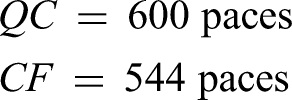
One of the simpler problems, Problem 12 in Chapter 5, is translated in Appendix 4.2: A man walks from Q to C and then to F in Figure 8; he has walked a total of 1,144 paces. Another man walks from G to T and then to F; the difference between these two walks is 56 paces. The diameter of the circular city is required. Thus

$$QC+CF=1,144\mathrm{paces}$$

(2)

$$FT\text{–}TG=56\mathrm{paces}$$

(3)

and d is required. Then follows one of Li Ye's 171 demonstrations of the manipulation of polynomials to solve non-trivial problems. While this is obviously not a real-world problem, the method was definitely used in solving real practical problems in ancient China (see e.g., Wagner, 2013).

Two non-obvious facts, stated in Chapter 1 (see Appendix 4.1.2), are used:

$$QC\text{–}CF=FT\text{–}TG$$

(4)

$$CK\times TG={\displaystyle \frac{1}{2}{d}^2}$$

(5)

These follow from two facts stated in the Nine Chapters and proved by Liu Hui (Chemla and Guo, 2004: 726, 728–729; Guo et al., 2013: 1110–1121; Qian, 1963: 252–253; Shen et al., 1999: 494–495; Wagner, 2022):

$$d=QC+QT-CT={\displaystyle \frac{2\times QC\times QT}{QC+QT+CT}}$$

From these follow

$$QC=CT-QT+d=(CF+FT)-(TG+d)+d=FT-TG+CF$$

$$QC-CF=FT-TG$$

and

$$QC\times QT={\displaystyle \frac{1}{2}d(QC+QT+CT)}$$

$$CK\times TG=(QC-d)(QT-d)$$

$$=QC\times QT-d(QC+QT)+d^2$$

$$={\displaystyle \frac{1}{2}d(QC+QT+CT)-d(QC+QT)+d^2}$$

$$={\displaystyle \frac{1}{2}d\times QC+{\displaystyle \frac{1}{2}d\times QT+{\displaystyle \frac{1}{2}d\times CT-d\times QC-d\times QT+d^2}}}$$

$$=-{\displaystyle \frac{1}{2}d(QC+QT-CT)+d^2}$$

$$=-{\displaystyle \frac{1}{2}{d}^2+d^2={\displaystyle \frac{1}{2}{d}^2}}$$

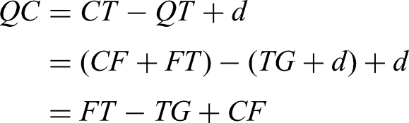
It follows immediately from (2), (3), and (4) that

$$\begin{array}{rl}& QC=600\mathrm{paces}\\ & CF=544\mathrm{paces}\end{array}$$

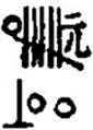
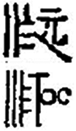
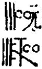
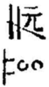
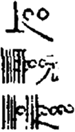
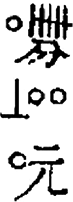
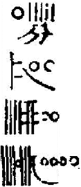
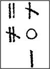
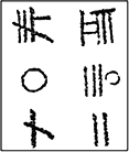
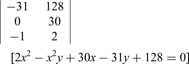
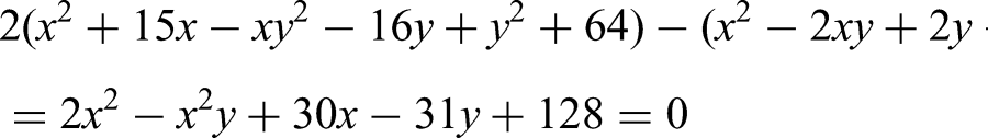
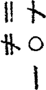
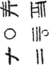
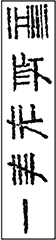
The polynomials are, as before, columns of counting-rod numbers. Representations of these are included directly in the text, as can be seen in Appendix 4.2. How these small drawings are to be interpreted is shown in Figures 9 and 10.

Figure 9.

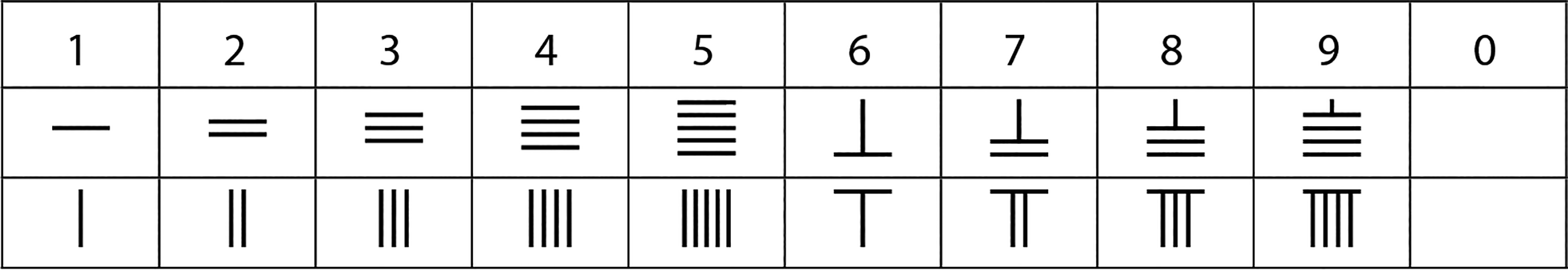
The two series of counting-rod numerals. Numerals of the two series are used alternately to allow closer spacing on the counting board.

Figure 10.

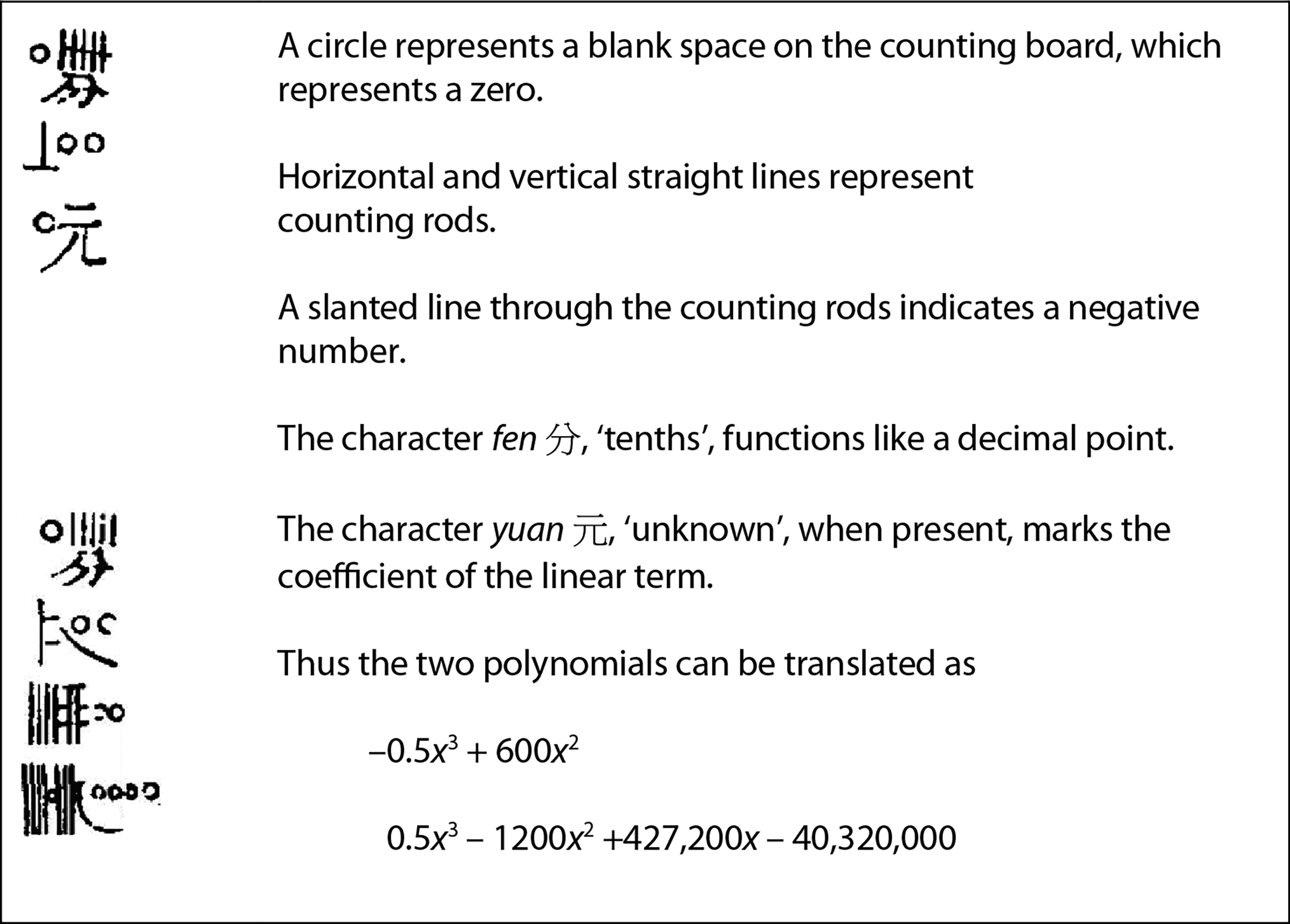
Two examples of the use of counting rods (chou 筹) to represent polynomials.

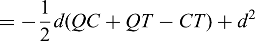
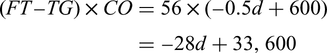
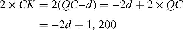
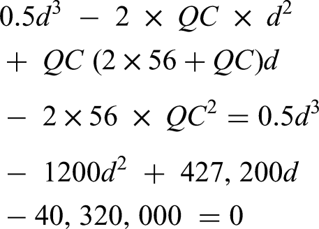
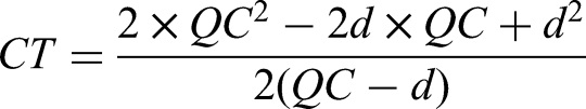
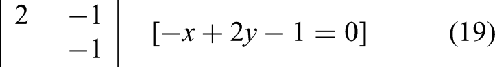
Li Ye's text gives first the calculation of the coefficients of the cubic equation to be solved numerically:

$$0.5d^3\text{–}1,200d^2+427,200d=40,320,000\mathrm{cubic}\mathrm{paces}$$

(6)

and gives the solution, 240 paces. Then follows the detailed derivation of this equation.

The first polynomial on the counting board is an expression for CO:

$$CO=QC\text{–}0.5d=\text{–}0.5d+600$$

(7)

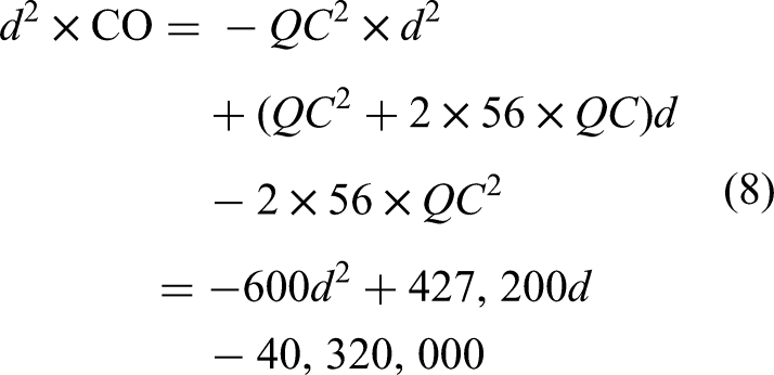
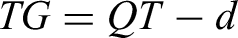
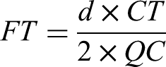
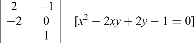
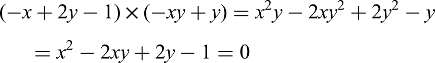
Next, an expression for FT is needed. Considering similar triangles, this is

$$FT={\displaystyle \frac{0.5d\times CF}{CO}}$$

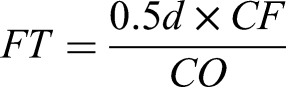
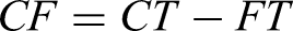
In the following steps, the divisor CO is ‘set aside’, so that the next polynomial is in effect

$$FT\times CO=0.5d\times CF=272d$$

Two further steps lead to an expression for TG:

$$(FT\text{–}TG)\times CO=56\times (\text{–}0.5d+600)=\text{–}28d+33,600$$

$$TG\times CO=(FT-[FT-TG])\times \mathrm{CO}=272d-(-28d+33,600)=300d-33,600$$

Now an expression for CK is needed, and the next polynomial is

$$2\times CK=2(QC\text{–}d)=\text{–}2d+2\times QC=\text{–}2d+1,200$$

Multiplying this by the expression found for TG and using (5) gives an expression for d²:

$$\begin{array}{rl}{d}^2\times \mathrm{CO}=& -Q{C}^2\times d^2\\ & +(Q{C}^2+2\times 56\times QC)d\\ & -2\times 56\times Q{C}^2\\ & =-600d^2+427,200d\\ & -40,320,000\end{array}$$

(8)

Now another expression for d² is needed. Using (7),

$$d^2\times CO=0.5d^3+600d^2$$

(9)

Subtracting (8) from (9) gives

$$\begin{array}{rl}& 0.5d^3-2\times QC\times d^2\\ & +QC(2\times 56+QC)d\\ & -2\times 56\times Q{C}^2=0.5d^3\\ & -1200d^2+427,200d\\ & -40,320,000=0\end{array}$$

which is equivalent to (6).

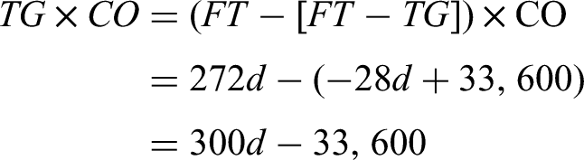
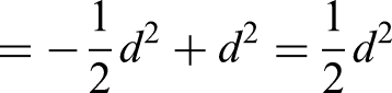
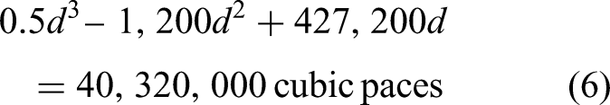
Confirming the problem solutions. The equation (6) has three roots: d = 168.737, d = 240, and d = 1,991.26. The third is clearly not a solution, since d > QC. The first two are solutions.

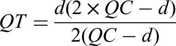
If QC and d are given, all of the other dimensions of the triangle are determined. From the Pythagorean Theorem and (4), the following can be derived:

$$QT={\displaystyle \frac{d(2\times QC-d)}{2(QC-d)}}$$

$$CT={\displaystyle \frac{2\times Q{C}^2-2d\times QC+d^2}{2(QC-d)}}$$

$$TG=QT-d$$

and, considering similar triangles,

$$FT={\displaystyle \frac{d\times CT}{2\times QC}}$$

$$CF=CT-FT$$

Then, given QC = 600, it can be calculated that both d = 168.737 and d = 240 can satisfy (2) and (3).

This example shows us the classical Chinese algebra of polynomials in one variable close to its full development, used in solving complex problems. The system clearly has limitations. In particular, Li Ye states all of his problems in geometric terms, the unknown quantity is in each case a linear measure, and all of his polynomials are functions of this unknown.

5. Zhu Shijie's Jade Mirror

In the Siyuan yujian (四元玉鉴, Jade Mirror of Four Unknowns, ⁷ published in 1303, hereafter Jade Mirror), we see the classical Chinese algebra of polynomials at its highest level of sophistication. Here, the columns of numbers representing polynomials in one unknown that we have seen in Li Ye's Sea Mirror are extended to rectangular arrays of numbers, which represent polynomials in up to four unknowns. The author, Zhu Shijie (朱世杰), appears to have drawn on several earlier works, but these are no longer extant (Du, 1966: 168).

In Li Ye's polynomials, the single unknown is called tianyuan yi (天元一) or simply tianyuan, the ‘celestial unknown’. In Zhu Shijie's book, the unknowns are called tianyuan (天元), diyuan (地元), renyuan (人元) and wuyuan (物元), the ‘celestial’, ‘terrestrial’, ‘human’ and ‘creature’ unknowns. Modern scholars studying the Jade Mirror represent these with x, y, z and u.

In his book, Zhu Shijie introduces his methods with four worked examples, using one, two, three and four unknowns respectively. These have been translated several times (see Vanhée, 1931; Hoe, 1977, 2007; Guo et al., 2006: 42–85). This introduction is followed by statements of 284 problems with the barest of hints as to how they are to be solved. Fortunately, the Qing scholar Luo Shilin (罗士琳; 1789‒1853), in his Siyuan yujian xicao (四元玉鉴细草), published in 1837, gives detailed working (xicao) for each of them, and I depend heavily on his work in my discussion.

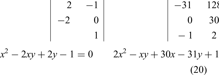
The counting-rod array notation for a polynomial in two variables is a rectangular array with a place for each coefficient, like this:

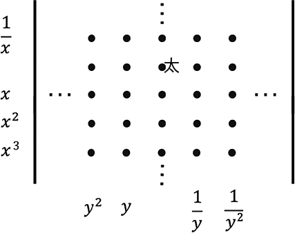
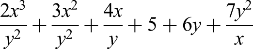
So that, for example, this array:

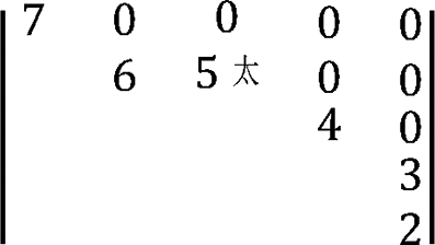would represent the polynomial

$${\displaystyle \frac{2x^3}{y^2}+{\displaystyle \frac{3x^2}{y^2}+{\displaystyle \frac{4x}{y}+5+6y+{\displaystyle \frac{7y^2}{x}}}}}$$

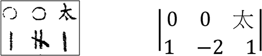
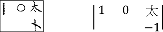
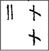
The use of counting-rods is in general the same as laid out in Figures 9 and 10. In illustrations of polynomials in the book, the constant term is often but not always marked with the character tai (太, ‘supreme’). The calculator might have marked this on the counting board in some way, or he might simply have kept the position in mind.

This notation appears to be perfectly general for polynomials in two unknowns. Extending it to a general notation for polynomials in three or four unknowns, however, would seem to require three- or four-dimensional arrays. In these cases, Zhu Shijie uses a complex notation which I do not understand deeply enough to explain properly, and in the following, I shall be concerned only with the case of two unknowns.

It is apparent that the array notation owes much to the matrix approach to systems of linear equations presented in the Nine Chapters, Chapter 8. ⁸ The terms xiao (消, ‘clear’) and qi (齐, ‘homogenize’) are used here in ways analogous to their use there.

Multiplying or dividing an array by x is done simply by moving the whole array down or up. The same operations with y move the array to the left or right. This moving of the array requires only moving the character tai (太; or other indication of the constant term) accordingly.

The algorithm for multiplication of two arrays is never stated, but its result is of course the array corresponding to the product of the polynomials represented by the multiplicand arrays.

Each of the 288 problems in the book gives two equations, the first prefaced by jin you (今有, ‘now there is …’), and the second by zhi yun (只云, ‘it is only stated that …’). In Zhu Shijie's four worked examples, two equations are developed that correspond to these, called the jin array and the yun array. From these are developed the ‘left’ and ‘right’ arrays, corresponding to two polynomials which are both equal to zero. These are analogous to the matrices in the linear algebra of the Nine Chapters; the operations of ‘homogenizing’ and ‘clearing’ are used to eliminate all unknowns except x. The Chinese version of Horner's method is then used to find a numerical root of this equation.

With only two equations given in each problem, how are problems of three or four unknowns solved? Most or all of these involve right triangles, and an implicit third equation is the Pythagorean Theorem. And the worked example using four unknowns has only three actual unknowns, the three sides of a right triangle.

The example of a problem in two unknowns that I have chosen for this discussion is Problem 15 of Section 6. ⁹ It is translated, together with Luo Shilin's detailed working, in Appendix 5.

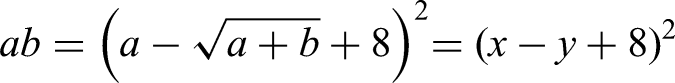
Letting a and b be the dimensions of a rectangle, the statements of Problem 15 amount, in modern notation, to

$$\sqrt{ab}+\sqrt{a+b}-a=8\mathrm{paces}$$

(10)

$$\sqrt{a+b}-\sqrt{b}=1\mathrm{pace}$$

(11)

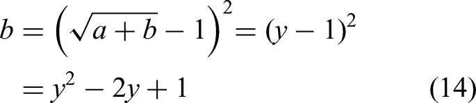
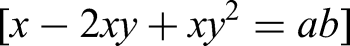
Zhu Shijie directs the reader to let the two unknowns be

$$x=a,y=\sqrt{a+b}$$

(12)

and ‘calculate by combining’ these. He then gives the numerical coefficients of the final polynomial equation to be solved,

$$x^4-4x^3-26x^2-196x+225=0$$

(13)

together with the result a = 9 paces, b = 16 paces. He does not indicate how these coefficients are calculated, leaving to the reader the task of getting from (10) and (11) to (13).

Fortunately, Luo Shilin gives all the details. Using modern notation, from (11),

$$b={\left(\sqrt{a+b}-1\right)}^2=(y-1{)}^2=y^2-2y+1$$

(14)

Further, from (10),

$$ab={\left(a-\sqrt{a+b}+8\right)}^2=(x-y+8{)}^2$$

$$=x^2+16x-2xy-16y+y^2+64$$

(15)

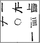
Luo Shilin expresses these polynomials as arrays:

Multiplying (14′) by x gives

$$[ab=x-2xy+x{y}^2]$$

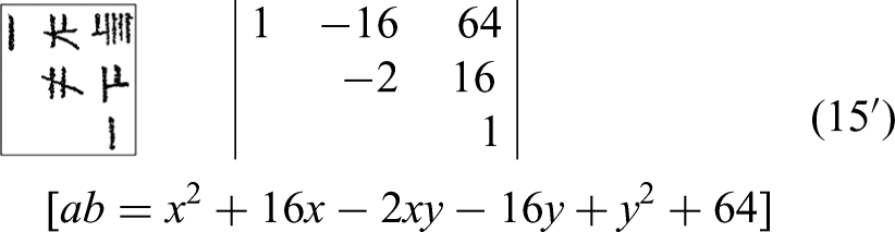
Subtracting (16) from (15′),

$$\left|\begin{array}{c}\begin{array}{ccc}1& -16& 64\\ -1& 0& 15\\ & & 1\end{array}\end{array}\right|[x^2+15x-x{y}^2-16y+y^2+64=0]$$

(17)

This he calls the jin 今 array. Further, from (11),

$$[b=-x+y^2]$$

Subtracting (14′) from (18) gives

$$\left|\begin{array}{cc}\begin{array}{c}2\\ \end{array}& \begin{array}{c}-1\\ -1\end{array}\end{array}\right|[-x+2y-1=0]$$

(19)

This he calls the yun (云) array.

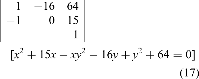
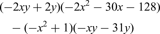
Luo Shilin has now arrived at two polynomials in x and y, (17) and (19), each of which equals zero. The next step is to eliminate the two y² terms in (17). Multiplying the yun array by the left column of the jin array, (17),

$$\left|\begin{array}{cc}\begin{array}{c}2\\ -2\\ \end{array}& \begin{array}{c}-1\\ 0\\ 1\end{array}\end{array}\right|[x^2-2xy+2y-1=0]$$

$$\begin{array}{rl}& (-x+2y-1)\times (-xy+y)=x^{2}y-2x{y}^2+2y^2-y\\ & =x^2-2xy+2y-1=0\end{array}$$

This is called the ‘left’ array. To make the ‘right’ array, the jin array, (17), is doubled and the ‘left’ array is subtracted from it,

$$\left|\begin{array}{cc}\begin{array}{c}-31\\ 0\\ -1\end{array}& \begin{array}{c}128\\ 30\\ 2\end{array}\end{array}\right|[2x^2-x^{2}y+30x-31y+128=0]$$

$$\begin{array}{rl}& 2(x^2+15x-x{y}^2-16y+y^2+64)-(x^2-2xy+2y-1)\\ & =2x^2-x^{2}y+30x-31y+128=0\end{array}$$

On the counting board are now the ‘left’ and ‘right’ arrays:

  

$$\begin{array}{rl}& \left|\begin{array}{cc}\begin{array}{c}2\\ -2\\ \end{array}& \begin{array}{c}-1\\ 0\\ 1\end{array}\end{array}\right|\left|\begin{array}{cc}\begin{array}{c}-31\\ 0\\ -1\end{array}& \begin{array}{c}128\\ 30\\ 2\end{array}\end{array}\right|\\ & x^2-2xy+2y-1=02x^2-xy+30x-31y+128=0\end{array}$$

(20)

and the next step is to eliminate the four y terms. In this arrangement, the product of the ‘inner’ columns is subtracted from the product of the ‘outer’ columns:

$$\begin{array}{rl}& (-2xy+2y)\times (2x^2+30x+128)\\ & -(x^2-1)\times (-x^{2}y-31y)\\ & =x^4-4x^3-26x^2-196x+225=0\end{array}$$

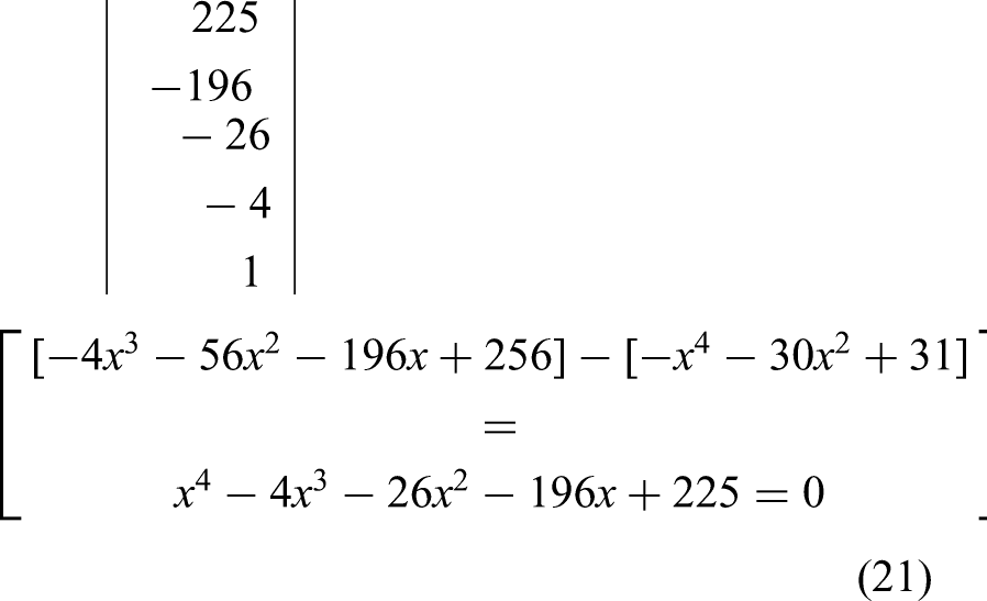
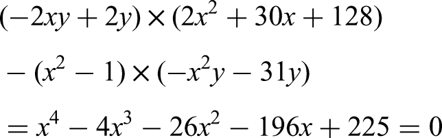
This result is (13), the equation given by Zhu Shijie to be solved numerically. It has two real roots, x = 1 and x = 9; and a = x = 9 is the correct solution. Luo Shilin does not indicate how b is calculated, but one simple way is to substitute a = 9 paces into (10) and (11) and take their difference, giving the result b = 16 paces. The root x = 1 is not a solution, as no value of b can in that case validate both (10) and (11).

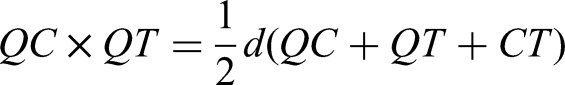
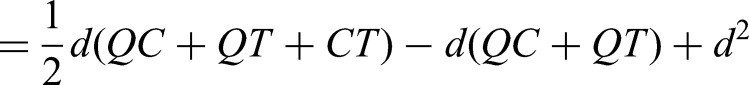
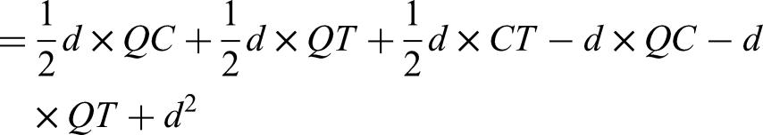
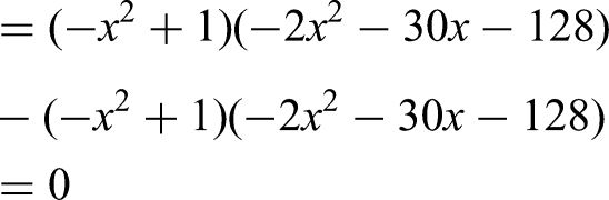
The calculation in (13)–(21) needs some explanation. It follows from the equations in (20) that

$$-2xy+2y=-(x^2-1)$$

$$-xy-31y=-(2x^2+30x+128)$$

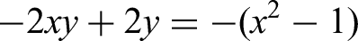
And the difference of the products of the inner and outer columns in (20) is

$$(-2xy+2y)(-2x^2-30x-128)-(-x^2+1)(-xy-31y)$$

$$\begin{array}{rl}& =(-x^2+1)(-2x^2-30x-128)\\ & -(-x^2+1)(-2x^2-30x-128)\\ & =0\end{array}$$

This example shows something of the sophistication that the algebra of polynomials reached in Zhu Shijie's book. Polynomials in more than one variable are allowed, the tie to geometry is entirely broken, and variables can point to functions of the unknown as in (10), $y=\sqrt{a+b}$ .

6. Concluding remarks

We have seen in this article examples from four books ranging over more than a millennium. What can we say about the conceptual development that they show?

It is important to emphasize that more examples, from more books, would undoubtedly lead to more solid insights. Furthermore, there were many other mathematical books written and published in our period of interest, most of which are no longer extant. And we must also assume that there were many mathematicians who contributed to this development but never wrote a book and whose names we do not know. Therefore, while we naturally admire the accomplishments of Liu Hui, Wang Xiaotong, Li Ye and Zhu Shijie, we may not suppose that they alone moved the development forward.

The example from the Nine Chapters, with Liu Hui's commentary, showed that a well-known technique could be used for more than it was designed for—this is often the first step in the evolution of a technique or a technology. But as long as the technique of root extraction was conceptually tied to geometry, Problem 20 remained an interesting curiosity without practical application or obvious potential for further development.

The first major development that we see through these examples is the recognition in Wang Xiaotong's Continuation that the column of numbers used in the root-extraction process is what we would call an equation: it is in effect a statement that performing certain operations on an unknown quantity results in a certain quantity.

Wang Xiaotong formed his equations by ad hoc geometric constructions, so his algebra was still tied to geometry, but while Liu Hui saw the ‘coefficients’ of his ‘equation’ as areas or volumes, for Wang Xiaotong, they are simply numbers that appear in the calculation of certain volumes. ¹⁰

In the example from Li Ye's Sea Mirror, we see a break in the connection to geometry. Though all of the problems in the book are stated in geometric terms, the actual calculations are entirely concerned with numbers.

Further, in this book, a column of numbers is not always an equation to be solved numerically, but an expression for one unknown in terms of another. These expressions can be manipulated: added to, subtracted from, or multiplied by other expressions, or multiplied or divided by a constant. Looking only at the first steps in the example, the equation (7) states a relation between CO and d. The aim of the manipulations is to derive an expression in the unknown which is equal to zero. This is then an equation that can be solved numerically. The general method seems to be to find two different expressions in the unknown for the same variable and subtract the one from the other; in our example, equations (8) and (9), two expressions for $d^2\times CO$ .

In Zhu Shijie's Jade Mirror, we see the highest level of sophistication that was reached in this algebraic system. It is extended to deal with up to four variables, manipulated using methods inspired by the matrix algebra of the Nine Chapters. ¹¹ An advance that has received less attention is greater freedom in the choice of variables. In Li Ye's Sea Mirror, the variable in each polynomial expression is the unknown quantity of the respective problem. In the Jade Mirror, a variable can be a function; in our example, the variable $y=\sqrt{a+b}$ (see equation (12)). While Zhu Shijie has no general symbolism for a function like $\sqrt{a+b}$ , and must state the calculation in words, he is able to deal with it by implicitly ‘reasoning about calculations’, as Wang Xiaotong before him had done in some cases (Lim and Wagner, 2017: 51–52).

What were these books? Were they textbooks of practical mathematics? While their examples are often not at all practical, the mathematics that they present was definitely used in practical problem-solving (Lim and Wagner, 2017: 12; Wagner, 2013, 2023: 71–75). Both the Nine Chapters and Wang Xiaotong's Continuation were used in mathematical education in the Tang period (Lim and Wagner, 2017: 13–20), and presumably later as well; but the Sea Mirror and the Jade Mirror seem not to have been used as textbooks. Perhaps they should be categorized as ‘pure mathematics’ or ‘recreational mathematics’—though these are modern concepts, not necessarily applicable to ancient books.

Why was this marvellous algebra of polynomials totally forgotten by the late fourteenth century, the beginning of the Ming dynasty? No book later than Zhu Shijie's Jade Mirror mentions it before the renewed interest of Chinese mathematicians in the nineteenth century. The introduction of the abacus around this time may be part of the explanation, together with revised administrative practices in public works. It also seems likely that ‘pure mathematicians’ had developed the system as far as it could be taken without a radical paradigm change, and therefore turned to other interests.