
Abstract
We propose a Mahalanobis distance–based Monte Carlo goodness of fit testing procedure for the family of stochastic actor-oriented models for social network evolution. A modified model distance estimator is proposed to help the researcher identify model extensions that will remediate poor fit. A limited simulation study is provided to establish baseline legitimacy for the Mahalanobis distance–based Monte Carlo test and modified model distance estimator. A forward model selection workflow is proposed, and this procedure is demonstrated on a real data set.
Introduction
Social networks define an important type of data structure that has been gaining attention in recent years. Social networks are dyadic relations between social actors (e.g. individuals, organizations, or teams). Important examples are affective relationships such as trust and friendship, or task-oriented relationships like advice seeking. Networks are commonly represented by directed graphs or more complicated structures, where the nodes in the graph represent the social actors and the arcs (directed) or edges (non-directed) represent the ties between them. A classical textbook is Wasserman and Faust (1994), and recent textbooks are, for example, Kolaczyk (2009) and Borgatti et al. (2018).
For the study of network dynamics, Snijders (2001) introduced stochastic actor-oriented models (SAOMs), and proposed estimators for parameters in these models given network panel data using the method of moments (MoM). Bayesian estimators were proposed by Koskinen and Snijders (2007) and maximum likelihood estimators by Snijders et al. (2010a). The model was extended to the coevolution of networks and actor-level variables (Snijders et al., 2007; Steglich et al., 2010) and to the evolution of multivariate networks (Snijders et al., 2013). It is implemented in the R package RSiena (Ripley et al., 2019) and has been widely applied in the social sciences (e.g. Veenstra et al., 2013). An overview is given in Snijders (2017).
Compared with these developments, issues of model selection have not been elaborated in as much detail. Model selection for SAOMs usually proceeds guided by research questions, and utilizing substantive knowledge combined with forward model selection and hypothesis testing (Lospinoso et al., 2011; Schweinberger, 2012). Some guidelines were given in Snijders et al. (2010b), but not propped with formalized methods. This article proposes methods for assessing goodness of fit (GOF) of estimated models, thereby complementing the existing methodology.
In the statistical tradition of GOF (cf. Lehmann and Romano, 2005), we consider evidence as to whether the observed data is consonant with the assumption that it came from the fitted model under study. Hypothesis testing focuses on a specific alternative hypothesis. In contrast, the proposed GOF method has no particular alternative in mind. It evaluates how well the model fits in general. Because of the complex nature of network data, we do not think an omnibus GOF test is feasible. Therefore, we focus on a wide set of features for which a good fit between model and data is desirable, and study the correspondence for these features by Monte Carlo methods, much as was done by Hunter et al. (2008) for GOF studies for non-longitudinal network modeling.
We propose a data-driven methodology for assessing the fit between data and model based on a set of features that may be chosen by the user, but for which we make some suggestions, and we propose methods assisting the data analyst to find the directions, within a larger set of options, that seem most promising for improving the model fit if it is found to be lacking. These empirical considerations must be used in practice together with considerations based on substantive theories and whatever is available as knowledge of the processes determining network change; data-driven procedures can supplement, but not supplant, subject-matter knowledge.
The ideal for network modeling is that by specifying rules for network formation based on local information, the global properties of the network will also be represented in a satisfactory way. Local properties depend on neigbourhoods of the nodes, that is, other nodes directly connected (by incoming or outgoing ties) or connected through at most one intermediary. Examples of local properties are reciprocation, characteristics of tied nodes, and the frequency of various triadic configurations (Holland and Leinhardt, 1976). An example of a global property is the frequency distribution of geodesic distances, the geodesic distance between two nodes being defined as the minimum length of a path connecting them. Thus, the stochastic models will be based on local information, while the features used for checking will be based on local as well as global information.
The estimation method mainly used for SAOMs is the MoM, because it is much less time-consuming than likelihood-based approaches. Fit comparison based on likelihoods, therefore, is not available in many practical situations, and will not be considered here. Instead, fit assessment will be based on comparing features of the observed network to their expected values in the estimated distribution of networks, estimated from a large number of simulations. When this assessment leads to a conclusion of poor fit, it is desirable to remediate this by proposing model elaborations. Estimation is computationally intensive, and testing large numbers of candidate models can be time-consuming. Therefore, we also propose a computationally cheap predictor for the improvement of fit if the model were to be extended by specific additional effects. This estimator can be evaluated using only ingredients calculated already for the MoM estimation of the restricted model.
This article proceeds by first providing a brief introduction to SAOMs. We then present some possibilities for GOF features, which we call auxiliary statistics. Next, we propose a Monte Carlo–based GOF test based on the auxiliary statistics. Most interesting auxiliary statistics are multi-dimensional; they are therefore combined using the Mahalanobis distance (Mahalanobis distance–based Monte Carlo (MDMC)). A computationally cheap estimator for the Mahalanobis distance that would be obtained from specific model extensions, based on a first-order Taylor series, is developed to give suggestions to the researcher for choosing model extensions to remediate lack of fit, the so-called modified model distance (MMD) estimator. A set of simulation studies is conducted to demonstrate the effectiveness of both the GOF test and of the MMD estimator. The proposed GOF procedure is summarized in a workflow. This workflow is demonstrated in a brief forward model selection exercise. The article concludes with a discussion on some future directions.
This MDMC approach was proposed in the conference paper Lospinoso and Satchell (2011) and the unpublished DPhil dissertation Lospinoso (2012), and has already been widely applied. However, until now it was not formally described in a publication. The MMD estimator was not yet described or applied in other publications (except for the mentioned dissertation). The simulation studies are new.
Stochastic actor-oriented models
We present the model as developed in Snijders (2001); see Snijders (2017) for a treatment focusing on statistical issues and Snijders et al. (2010b) for a friendly introduction. A social network composed of n actors is modeled as a directed graph (digraph) with nodes
The network is observed at discrete time points called observations occurring at times
The model assumes that the social network evolves in continuous time over an interval
The stochastic process
The SAOMs consider two principal concepts in constructing the intensity matrix: the frequency at which actors i get opportunities to update one of their outgoing tie variables
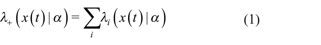
where
Rate functions may depend on actor-level covariates and the network position of actors. For simplicity, we here consider rate functions depending on neither i nor x, but only on the period, that is,
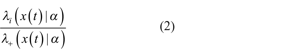
Now suppose that an opportunity for change arises for actor i, while the current digraph is x. Define
where
The selection of the tie variable
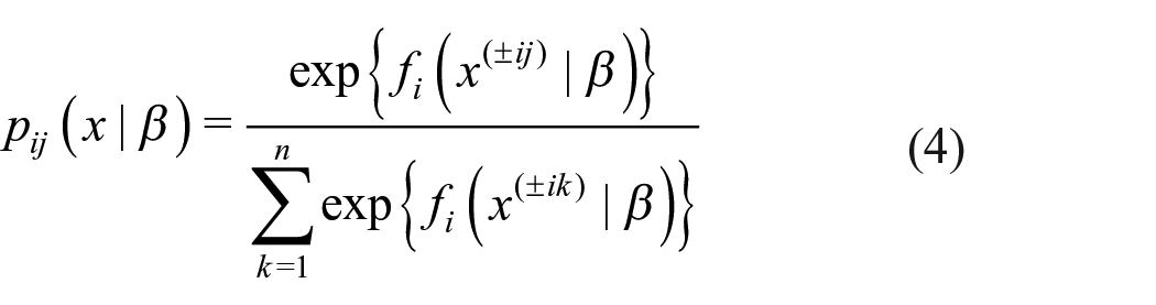
In accordance with the formal definition
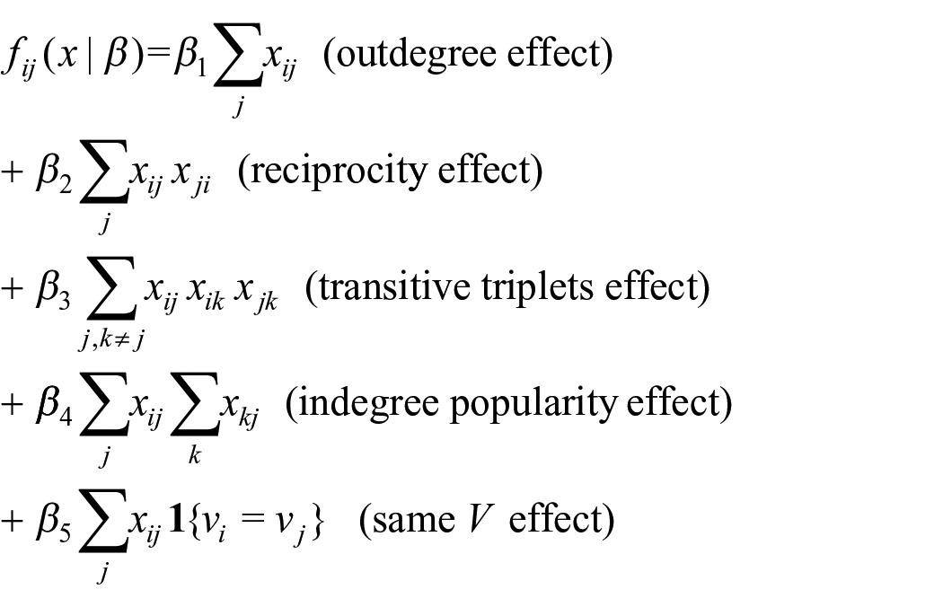
A basic menu of effects
1. Outdegree effect
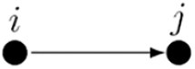
represents the tendency for actors to have outgoing ties. This parameter is analogous to a constant term in regression models. In practice, it is always included in the model to fit the trend in the total number of ties.
2. Reciprocity effect
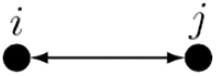
represents the tendency for actors to reciprocate incoming ties with outgoing ties.
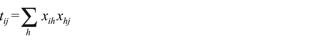
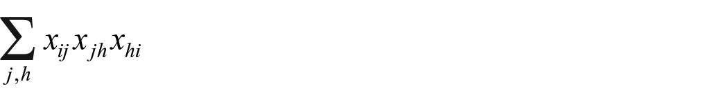
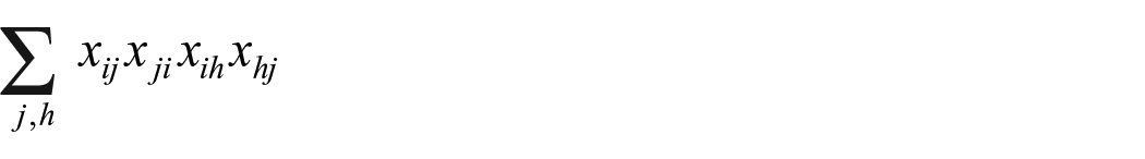
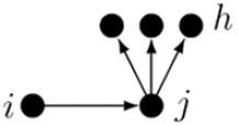
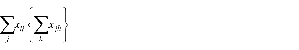
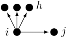
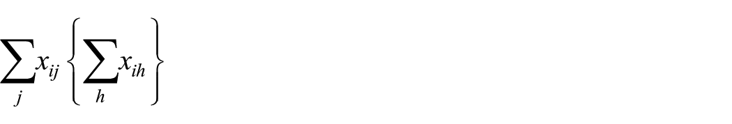
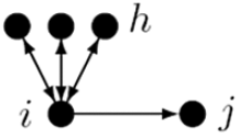
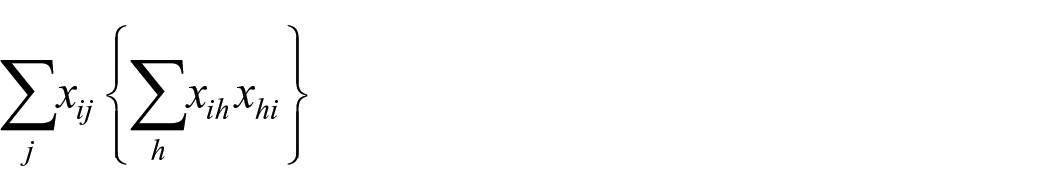
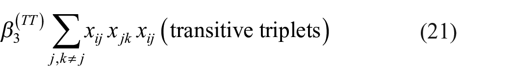
3. Transitive triplets
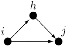
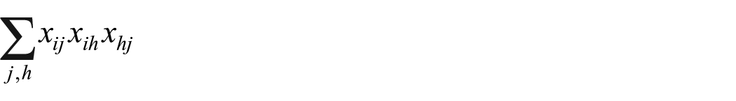
represents the tendency for an actor to create transitively closed structures, where “friends of friends are friends.”
4. Geometrically weighted shared partners (“gwesp”)
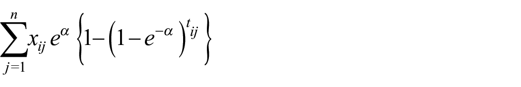
where
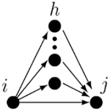
is another representation of the tendency to create transitively closed structures, where the number of indirect connections (“two-paths”)
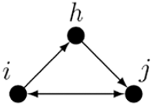
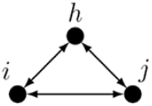
5. Three-cycles
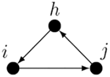
represents the tendency for an actor to create closed cycles
6. Transitive reciprocated triplets
is an interaction between reciprocity and transitivity (see Block, 2015).
7. Dense triads
represents the tendency for an actor to be a part of triads where everybody is mutually connected.
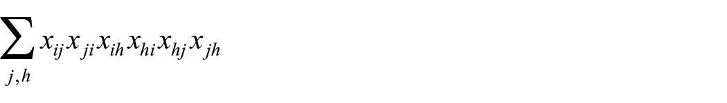
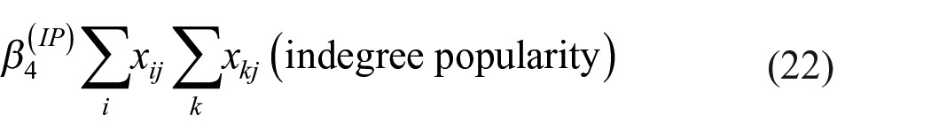
8. In-degree popularity

represents the tendency of actors to send ties to other actors with currently high in-degrees.
9. Out-degree popularity
represents the tendency of actors to send ties to other actors with currently high out-degrees.
10. Out-degree activity
represents the tendency of actors with currently high out-degrees to create new ties.
11. Reciprocated-degree activity
represents the tendency of actors with currently many reciprocated ties to create new ties.
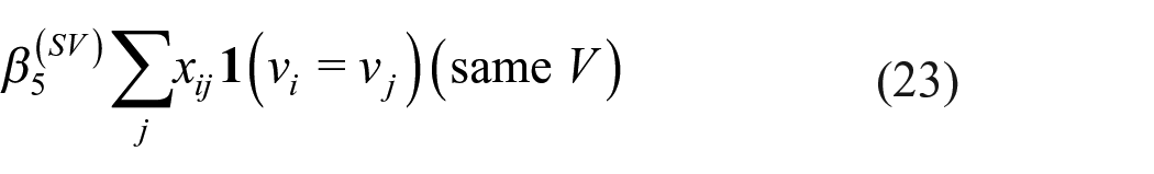
12. Same covariate
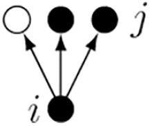
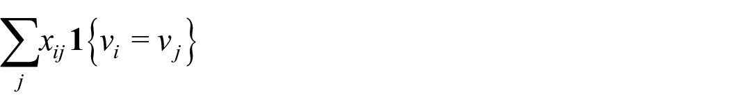
for a categorical actor covariate V, where
13. Similar covariate
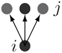
for a numerical actor covariate V represents the tendency of actors to create ties to other actors that have a similar value of this covariate.
Some of these effects can have seemingly similar consequences for the generated networks. For example, transitive triplets, gwesp, dense triads, and the same or similar covariate effects all will lead to some kind of clustering in the network. One of the purposes of the GOF studies is to determine which of these provides the best fit.
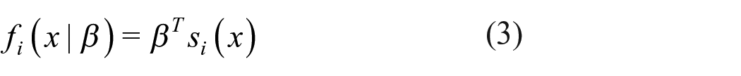
The mostly used estimation method for these models is the MoM (Snijders, 2001, 2017). Denoting the parameter by
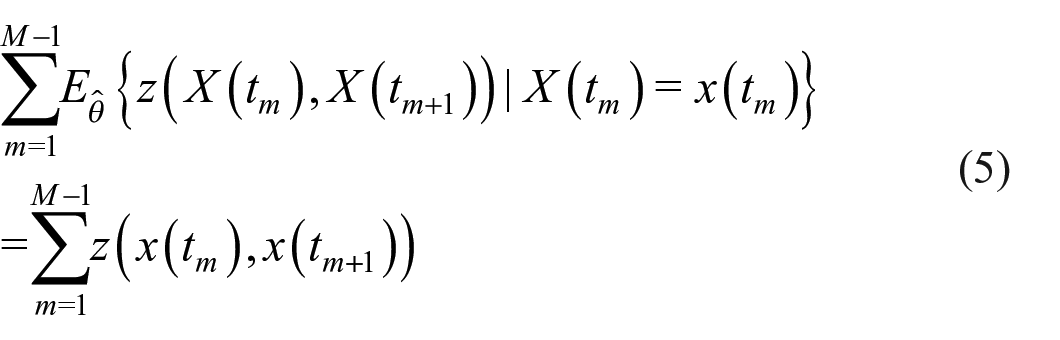
for a suitable vector of statistics z, which are sensitive to the parameters in
which are sensitive to the rate parameters
which is sensitive to the parameter
Statistics
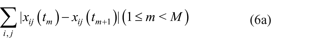
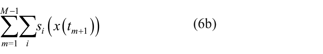
The “GOF” problem is one of testing the hypothesis that the model which generated the observed data is equal to the fitted model. Due to (1) the vastness of the state space of networks and (2) the idea that we have a “sample of size 1” observed over time, the approaches that have been developed for standard statistical modeling cannot be applied. Here, we follow the approach proposed by Hunter et al. (2008) and used also by Robins et al. (2009) for assessing the GOF of exponentially random graph models representing cross-sectionally observed networks. Many of the statistics proposed below are adopted from, or inspired by their work. This approach takes one auxiliary statistic, which is a vector of features of the data that is not directly included in the model, that is, it is not a function of the estimation statistics (equation 6). The value of this auxiliary statistic is compared between the observed data and their distribution as implied by the SAOM with the estimated parameters. In practice, usually several auxiliary statistics will be considered; the explanation of the procedure is for one vector-valued auxiliary statistic.
Before proposing the form of the GOF test, we present a number of possible auxiliary statistics. This list is by no means exhaustive, but we provide concrete examples which will be used in the simulation study and the example application later in this article:
Triad census. There are 16 possible isomorphic subgraphs of three nodes and the
The triad census can be used to assess whether the nuances of local network structure, such as network closure (i.e. transitivity)—a fundamental feature of social networks—are accurately represented by the fitted model.
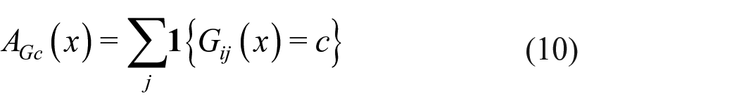
Edgewise shared partners (ESP). We can also consider, for a given C, the vector of statistics
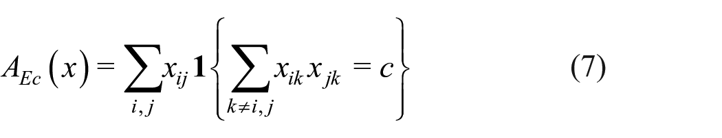
where
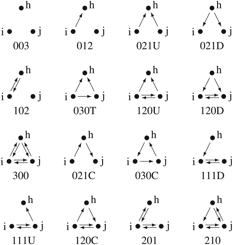
The 16 possible triads for transitivity in a digraph, adapted from Holland and Leinhardt (1976). The Mutual/Asymmetric/Null (MAN) notation for each triad is also given below each figure. For certain MAN classes, for example, 030C, a letter is appended to make the notation unique.
Outdegree distribution. This is the vector of statistics

These statistics count the number of nodes with c outgoing ties. In the social networks literature, this is often interpreted as the activity of the nodes. The dimension C of this statistic will be chosen based on the observed network and the interests of the researcher. While average outdegree is modeled explicitly by virtually all SAOM models used in practice, the distribution of outdegrees can have many different shapes, and these will not automatically be represented well by an estimated model.
Indegree distribution. This is the vector of statistics
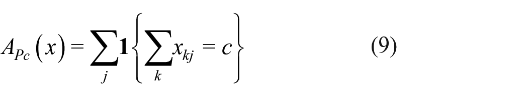
These elements count the number of nodes with c incoming ties, in the social networks literature often interpreted as popularity. Indegree and outdegree distributions are quite distinct from one another, and should be considered separately.
Geodesic distances. Define
The distribution of geodesic distances is an emergent property of social networks which is important, for example, for how quickly ideas and norms can spread. Importantly, geodesic distance is among the statistics presented here the only non-local characteristic of the network.
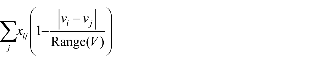
Edgewise similarity. Covariates are denoted
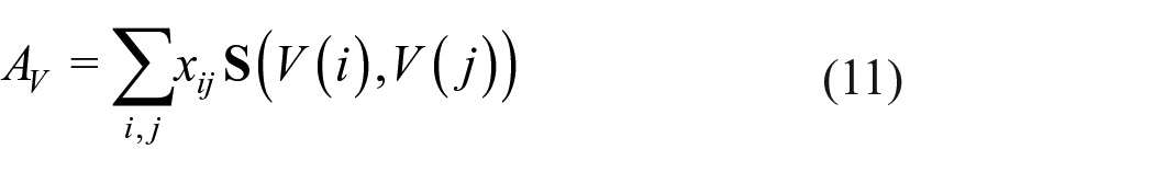
where
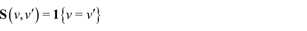
is a sensible choice. For numerical covariates, a transformed mean absolute difference can be used, as in
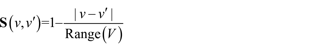
The choice of similarity function should depend on substantive theory and field knowledge, and on which aspects of fit are deemed important.
A Monte Carlo Mahalanobis distance based GOF test
In the previous section, we outlined a number of important features of digraph and covariate data that can be used for assessing GOF. From these auxiliary statistics, we now focus on only one GOF statistic
Recall that we assume to have panel data, that is, a sequence of observed networks
For simplicity, we deal with a single period. Since the estimation conditions on
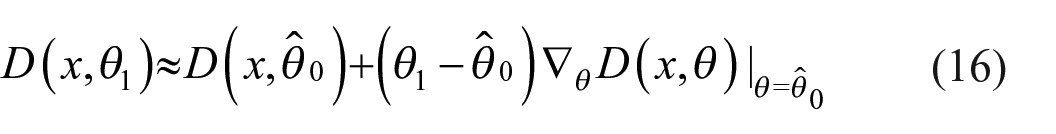
The approach taken here is to construct a function D that, for a given vector of statistics
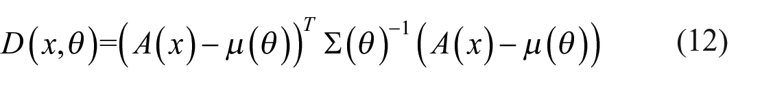
as our test statistic. We cannot in general compute equation (12) analytically; therefore, we use its Monte Carlo estimate
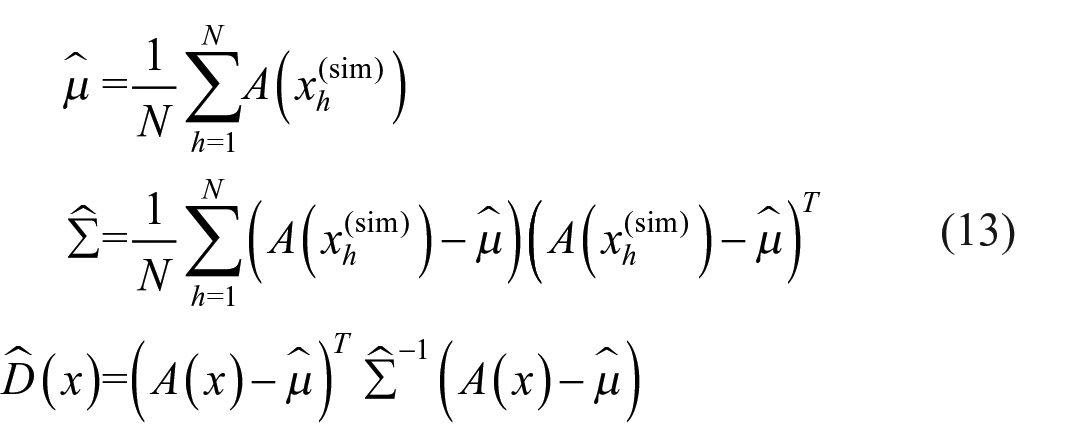
This
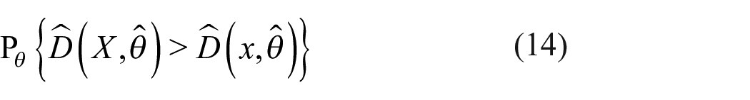
If the central limit theorem would apply, we would expect that equation (12) has approximately a chi-square distribution. However, we have no proof of this, and therefore follow a parametric bootstrap procedure. Then, plugging in the various values leads to
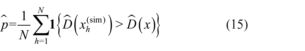
as the estimator for the p-value (equation (14)). A very low value indicates a poor fit.
For
Summarizing, this approach uses Monte Carlo simulations for parameter estimate
MMD estimator
The development of the MDMC allows the researcher to test GOF. If the fit is satisfactory, the researcher can go on with the analysis. In the event that fit is not acceptable, the researcher may have some theoretically based ideas on remediation. Even so, there may be a large number of effects that are plausible for inclusion. The richness and complexity inherent in networks provides the researcher with an enormous menu of effects to choose from, as is illustrated by the implemented effects in the RSiena package (Ripley et al., 2019). In most cases, theory and experience will not suffice to give a definite conjecture about the effect that should be added to improve the fit. Trying out many different effects will be time-consuming. This section presents an approximation to suggest which model improvements might be empirically promising, without requiring to estimate the correspondingly extended model.
The “MMD” estimator is an estimator for the Mahalanobis distance
The method proposed here is similar to methods used in model specification of structural equation models (SEMs) (cf. Kaplan, 1990, 1991). Specifically, they are to some extent analogous to the model modification index (MMI) of Sorbøm (1989) and the expected parameter change of Saris et al. (1987). An important difference with the use of the MMI in structural equation modeling is that in SEMs the GOF function (usually the log likelihood) is also maximized for obtaining estimates. This approach is unavailable to us in the current context. For MoM estimation, we have only an estimating function which cannot be used as a GOF function (for a MoM estimate, the estimating function is the difference between the left-hand and the right-hand sides of (5), and the estimate is defined by this being zero). Furthermore, the purpose of our GOF approach is to consider the fit specifically for statistics that were not used for the estimation.
For a given extension of the model, supposing it is the true one, denote the parameter value by
The question now is how to approximate the value
Letting
The gradient
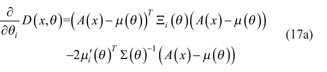
where
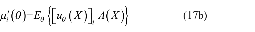
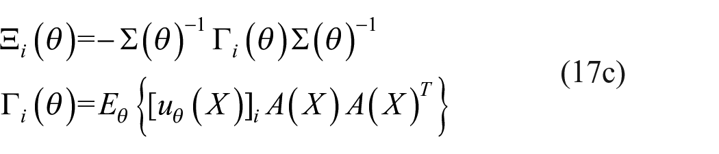
and
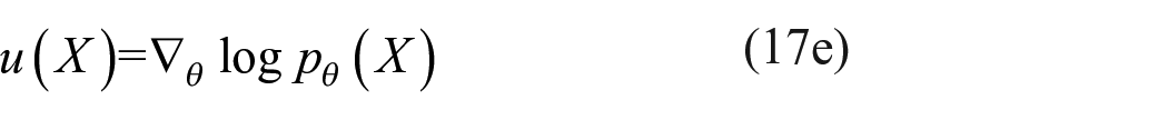
is the score function for the probability function
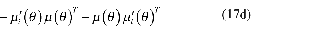
The derivatives are expressed in equations (17b) and (17d) using the score function
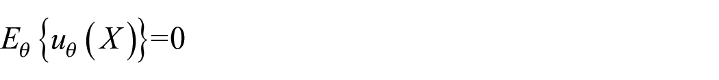
using the property that
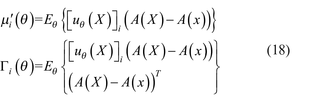
This leads to the Monte Carlo estimators
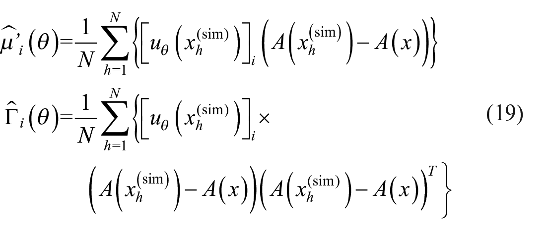
The MMD estimator for
Concluding, this approximation can be computed using simulations
Two warnings should be given here. First, the MDMC for an extended model does not need to be smaller than for the baseline model. This is because the MoM estimator is not oriented toward minimizing the function
For a given auxiliary statistic, when considering a set of potential model improvements, the improvement yielding the largest decrease in the Mahalanobis distance may be considered to be the best choice. Let us call this the MMD-1 model modification. We are just considering one-dimensional modifications, so there is no issue of different a priori advantages because of involving different degrees of freedom. A more subtle possibility is available when a set of several auxiliary statistics and a set of model improvements is under consideration. Then one may use the following procedure, to be called MMD-2, for model modification:
If all MDMC p-values are larger than some threshold, for example, the conventional
If for some auxiliary statistics the MDMC p-value is less than
Choose the effect that gives for this auxiliary statistic the best improvement as predicted by the MMD, and add this to the model.
Evidently, this procedure can be iterated.
Simulation study
In this section, we provide a small simulation study of (1) the validity and power of the proposed MDMC test, and (2) the effectiveness of the one-step Mahalanobis distance estimators in guiding model selection. We use a subset of the Teenage Friends and Lifestyle Study (TFLS) as the basis for our study. The TFLS data set was collected by West and Sweeting (1996) and utilized in many publications including Michell and Amos (1997), Pearson and Michell (2000), and Steglich et al. (2010). The panel data were recorded over a 3-year period starting in 1995, when the pupils were aged 13, and ending in 1997. A total of 160 pupils took part in the study, 129 of whom were present at all three measurement points. We utilize a subset of 50 girls from the study, called the TFLS-50, who were present at all three measurement points, chosen only for demonstration purposes, and distributed with the RSiena package (Ripley et al., 2019). Friendship networks were formed by allowing the pupils to name up to six best friends.
We simulate data in the following way: using the first observation of the TFLS-50 as the time-1 measurement, perform independent Monte Carlo simulations, according to three different SAOM specifications, each yielding 250 networks for the time-2 measurement. A binary actor covariate V is constructed, with values 0 for the first 25 and 1 for the last 25 girls. Since the order of the individuals in the data set is arbitrary, this is like a random covariate. We simulate with a constant rate
These 750 simulations are then used as the time-2 observation.
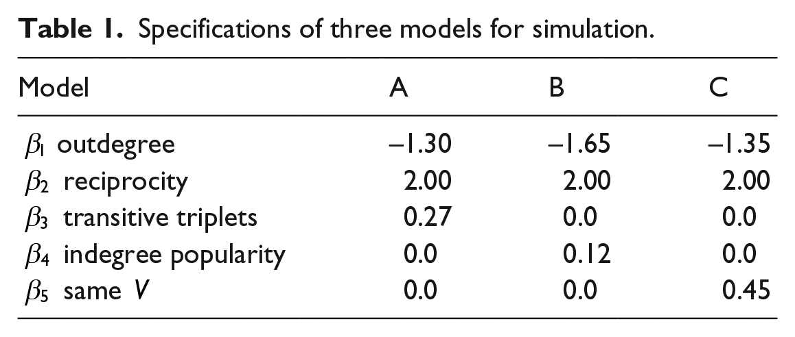
Three combinations of parameter values are used; in these combinations, one of the values
Specifications of three models for simulation.
In this demonstration, we use for the GOF study the following auxiliary statistics:
The triad census (see Figure 1);
The geodesic distance distribution for
The indegree distribution for
The outdegree distribution for
The number of Monte Carlo simulations to compute the
1. Estimate the parameters of an improperly specified base model with an incorrect evaluation function
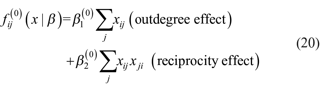
This may be considered to be a minimal model.
2. The proposed GOF test is evaluated at
3. Three model elaborations are considered. Each elaboration entails adding one of the following terms to the evaluation function
These effects were explained above. For each elaboration, the MMD is calculated. Note that for each simulated data set, one of these three is the properly specified model. The frequencies of selecting the correct model are reported. Using the MMD values, model selection procedure MMD-2 is applied.
4. As a sanity check, for the correct model we perform MoM estimation, and assess whether the estimates according to the properly specified model are close enough to the true parameter values.
5. For a new set of parameter values, we perform Steps 1–3 and evaluate the MDMC values
The results of these steps are as follows.
Step 1: estimation improperly specified model
Table 2 provides observed 95% intervals for
Frequency intervals for
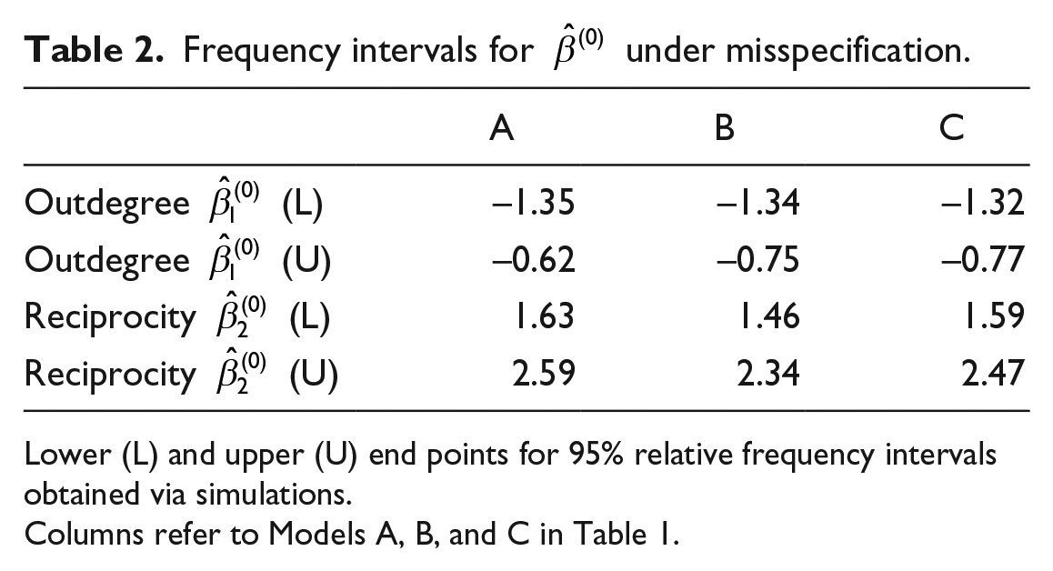
Lower (L) and upper (U) end points for 95% relative frequency intervals obtained via simulations.
Columns refer to Models A, B, and C in Table 1.
Step 2: perform the MDMC test
The proposed MDMC test is executed at the improperly specified model. Assembling the resulting tests into receiver operating characteristic (ROC) curves will allow us to investigate how well the test detects the misspecification. These curves tell us, for a specified false positive rate, the probability of rejecting the model. See Fawcett (2006) for more information on ROC curves. This is estimated here by calculating, for any given
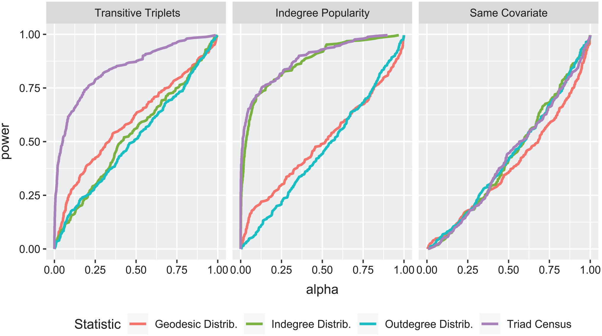
Receiver operating characteristic curve: the ROC curve gives indication of the power versus false positive (“alpha”) trade-off of MDMC using various auxiliary statistic specifications.
To interpret the conservative nature of the results of all auxiliary statistics for the same covariate effect, we point out two issues. These results suggest that misspecification with respect to covariates is not easily detected by auxiliary variables reflecting network structure; more research is needed to investigate whether this is generalizable. Other auxiliary statistics, considering specifically the occurrence of ties depending on the covariate values for sender and receiver, may be expected to have a better sensitivity for this type of misspecification. Second, insensitivity leads to conservativeness because the Mahalanobis
Step 3: MMD for candidate model elaborations
The most practically important characteristic of an MMD estimator is how often it would lead the researcher to select the appropriate model elaboration, given a misspecification. Table 3 gives the distribution of the rankings of MMD evaluated for each model elaboration. Again, the number of cases is 250, the number of simulated data sets.
Probability distribution of MMD rankings at Step 3.
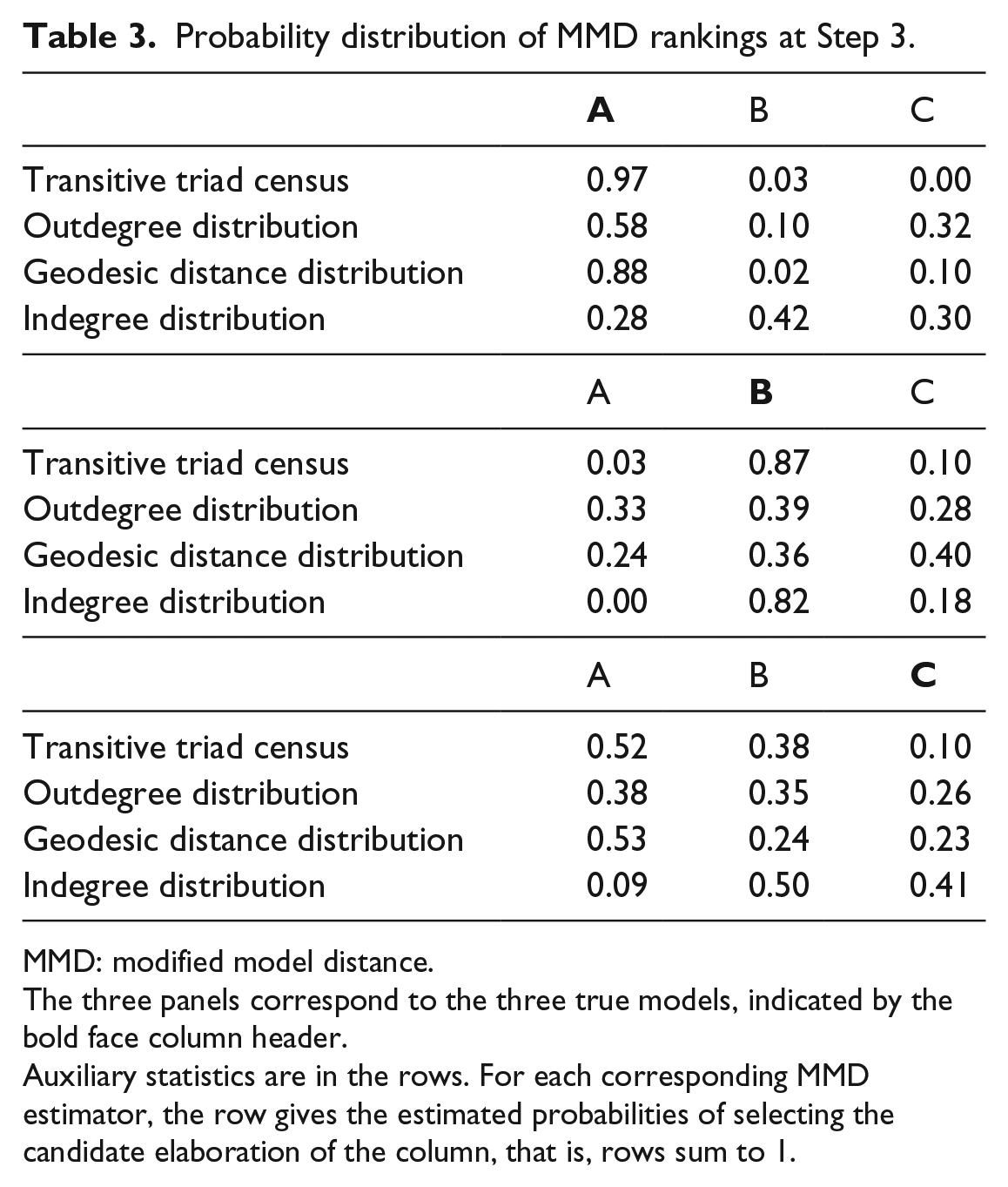
MMD: modified model distance.
The three panels correspond to the three true models, indicated by the bold face column header.
Auxiliary statistics are in the rows. For each corresponding MMD estimator, the row gives the estimated probabilities of selecting the candidate elaboration of the column, that is, rows sum to 1.
When the model misspecification is A, the omission of the transitive triplets effect (equation 21), the results in the first panel of Table 3 show that the MMD estimators based on geodesic distance, triad census, and outdegree distribution have the highest probability of selecting this model extension indeed. Only the indegree distribution selects more frequently the indegree popularity effect.
For the indegree popularity model B defined by equation (22), the triad census and the indegree distribution-based MMD estimators select the correct model more than 80% of the time. The results are much weaker for the geodesic and outdegree distributions, although for the latter the correct model still has the highest estimated probability.
The MMD estimator orderings for the same covariate model C, given by equation (23), do not perform well. None of the auxiliary statistics results in more than a 41% selection rate of the correct elaboration. This corresponds to the conservative nature for all auxiliary statistics for model C of the MDMC tests in Step 2.
The results of model selection procedure MMD-2 are given in Table 4. These are in line with the earlier results: the detectability of the transitive triplets effect and especially the indegree popularity effect are good, whereas the same covariate effect is not detectable by these auxiliary statistics. We remind the reader that the parameter values in the three cases were chosen so that the Wald test directed at this specific effect has a power of approximately 0.80. In this sense the effect sizes in the three cases are equally strong, and the difference in detectability depends on the correspondence between the auxiliary statistics and the misspecification, not on differences in effect size.
Relative frequencies of models selected by procedure MMD-2 in Step 3.
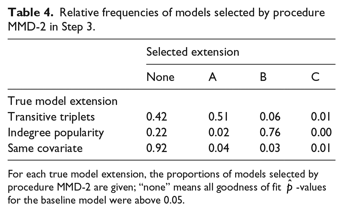
For each true model extension, the proportions of models selected by procedure MMD-2 are given; “none” means all goodness of fit
Step 4: MoM estimation of candidate models
During this step, we do a complete MoM estimation of each candidate model. All 95% coverage frequency intervals (not given for lack of space) include the true model parameters, a result in line with simulation studies of, for example, Snijders (2001) and Lospinoso et al. (2011).
Step 5: MDMC tests of candidate models
To assess the performance of the MMD estimator, we conduct a set of simulations varying the true extent to which one of the three model extensions is called for.
Define
For each data set, parameters are estimated under the base model (equation 20), and for each of the four auxiliary statistics, the MMD estimators for the three candidate models are calculated. Negative MMD values are truncated to 0. Then for each of the three candidate models, the full MoM estimation is carried through and the four Mahalanobis GOF MDMC statistics are computed. Thus, for each of the 600 data sets, there are 12 pairs of a MMD estimator and an MDMC statistic. To each of these pairs corresponds an MDMC value for the base model. The question now is, whether the MMD yields an adequate prediction of the improvement, that is, decrease, in the Mahalanobis distance when comparing the base model to the estimated candidate model. In other words, how good is the MMD as an approximation of the MDMC of the candidate model, where the MDMC of the base model can be used as a reference value.
Figure 3 presents the improvement of the Mahalanobis distance with respect to the base model, as realized (vertical axis) and as predicted by the MMD (horizontal axis). In the axis labels, MDMC(0) refers to the MDMC for the base model. The MDMC refers to the realized MDMC for the candidate model, and MMD refers to the MMD truncated to nonnegative values. In view of the skewness, all Mahalanobis distances were transformed by the square root.
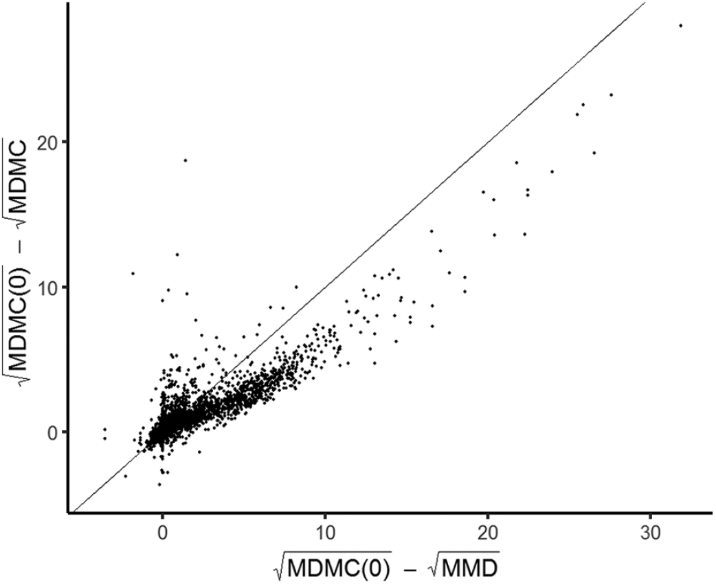
The decrease in Mahalanobis distance compared with the base model, as predicted by the MMD (horizontal axis) and as realized (vertical axis). The straight line indicates equality. All distances square root transformed; MMD left truncated at 0.
The figure shows a strong agreement. The realized improvements tend, however, to be smaller than the predicted improvements, as most points are below the equality line. The correlation between the differences MDMD—MDMC(0) and MMD—MDMC(0) is equal to 0.94, which is a confirmation of the value of this approximation.
Workflow
In this section, we suggest a possible GOF assessment approach for SAOM analysis that incorporates the MDMC testing procedure into the model fitting context. This can be carried out using the R package RSiena (Ripley et al., 2019), in which the MDMC test and the MMD estimator are implemented in the function sienaGOF.
First, we should point attention to time heterogeneity, which is a special kind of misspecification that is possible for data with
A proposed workflow is the following. The preceding remarks imply that the order of Steps 5, on the one hand, and 6–7 combined, on the other hand, is not fixed.
Select a provisional SAOM specification: this model should be parsimonious, based on the research question and existing knowledge about the processes driving the evolution of the network under study.
Reflect about time heterogeneity: if the data have three or more waves, and the average degree per wave has important jumps up as well as down, this is a sign of time heterogeneity for which it might be necessary to include time as a covariate. Whether this should be a linear time effect or some transformation of time depends on the pattern shown by the average degrees over the waves. One possibility is to include dummy variables for the waves.
In the case of three or more waves, if there is a suspicion of strong time heterogeneity, or if there is persisting lack of fit or lack of convergence, it is advisable to estimate by period, that is, for each pair of subsequent waves separately. This is possible only if the data set is large enough to make estimation by period feasible.
Estimate the parameters for the provisional model.
Check the convergence of the estimation: for MoM estimation, good convergence means that simulations drawn from the fitted model yield simulated values of the estimating statistics (6) that are very close to the observed values. The manual (Ripley et al., 2019) gives criteria. If convergence is poor, try re-estimating the model; the manual offers advice for how to proceed. If poor convergence is systemic, this may be evidence of poor agreement between the provisional model and the data. Experience has shown that systemic poor convergence may reflect, for example, that covariates should be included reflecting meeting opportunities (e.g. “same classroom” if the network is situated in a school context); or that additional degree-related effects should be included (e.g. reflecting isolated nodes); or that outdegree effects on the rate of change should be included; or that there is major time heterogeneity. In this case, the researcher should go back to Steps 1 or 2.
Check for time heterogeneity, if appropriate: if there are three or more waves, time heterogeneity can be tested using the function sienaTimeTest, as mentioned above, with remedial possibilities mentioned in Step 2.
Assess GOF with the proposed MDMC GOF test: the GOF test can be carried out for several auxiliary statistics. We recommend in any case to use the two degree distributions and the triad census, with the geodesic distances distribution as a valuable addition.
The GOF test provides a
If the observed
Extend the model, if the fit is inadequate: if the GOF test points out that the fit is not satisfactory, the model will have to be extended. The plot, further knowledge about the data, and theoretical considerations may point us to a list of candidate effects that could be added to the model. These candidate effects can be added directly to the model, or they may be evaluated approximately for their promise to improve fit by the MMD test described above. If there is a choice between several effects indistinguishable by theory, the one that yields the lowest MMD for the modified model may be chosen. The results of the simulation study above demonstrate that this is not a fail-safe procedure but it nevertheless can give meaningful guidance.
Iterate: depending on the results, some of the steps may have to be repeated.
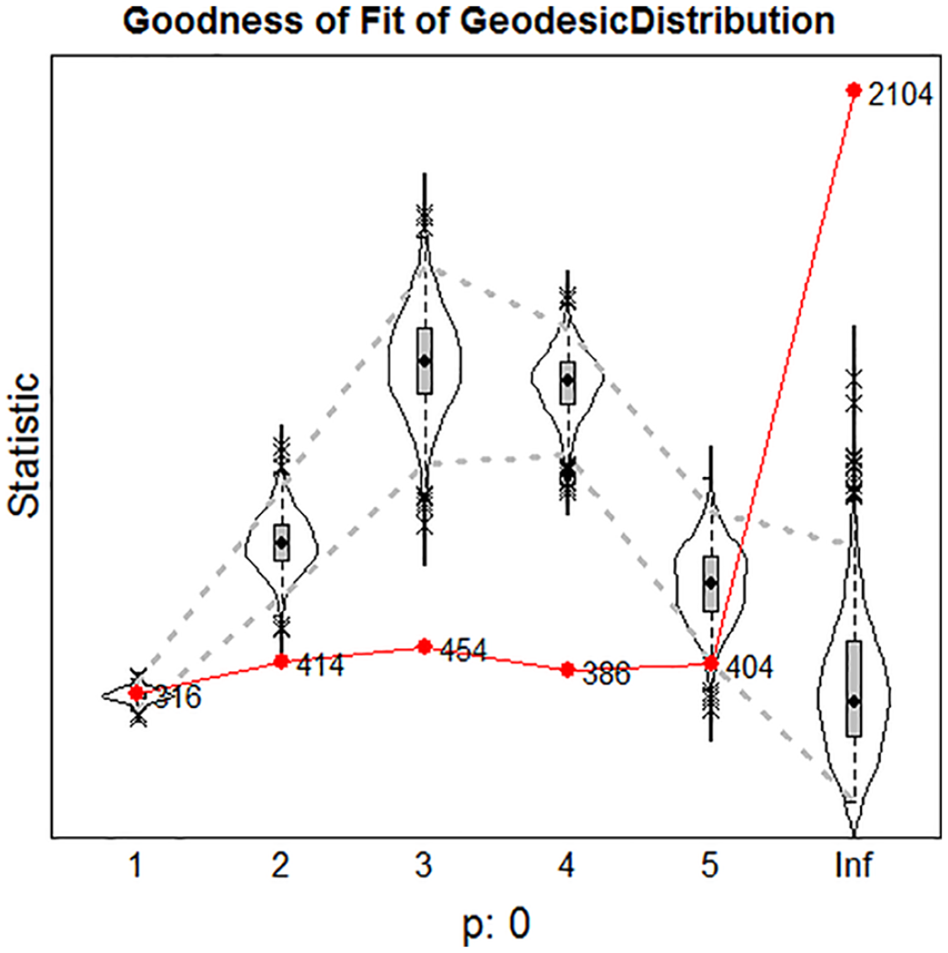
Goodness of fit diagnostic plot for the first model, with as auxiliary statistic the geodesic distance distribution. Observed values are indicated by numbers connected by a line. The simulated statistics are represented by the violin plots. Dotted lines give 95th percentile bands. The
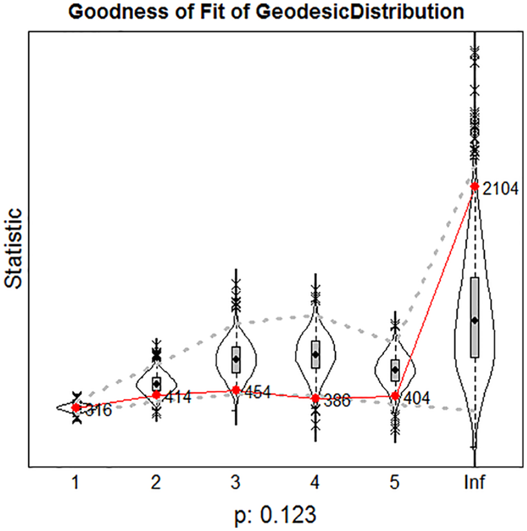
Goodness of fit diagnostic plot for the final model with as auxiliary statistic the geodesic distance distribution. Observed values are indicated by numbers connected by a line. The simulated statistics are represented by the violin plots. Dotted lines give 95th percentile bands. The
There are potential theoretical pitfalls here, however. (1) As with any model selection procedure, if it is applied without theory in mind, it will be much harder to defend the validity of the final model. (2) There may well be different possibilities for improving fit when it is found to be inadequate, so the result of this procedure may depend on random circumstances. (3) It may be desirable also to drop effects from the model at certain moments during the procedure—depending on theory and insight into the data; this is illustrated by the example below. Considerations about the research question and theoretical insights will always need to play a fundamental role.
Example
We provide a small example of our model fitting procedure applied to the subset of the TFLS data introduced above. The data set includes three observations of friendship networks and alcohol consumption habits (on a scale with values 1–5). We demonstrate a forward stepping model selection exercise, assuming—for the sake of this example only—that the researcher wishes to specify a priori only the reciprocity effect, has a list of candidate effects, and wishes to inductively select a set of effects that lead to an acceptable fit with respect to the indegree and outdegree distributions, the triad census, and the distribution of geodesic distances. “Acceptable” fit is defined by the usual 5% level for the MDMC
The list of candidate effects consists of transitive triplets, “gwesp,” three-cycles, transitive reciprocated triplets, dense triads, indegree popularity, outdegree popularity, outdegree activity, reciprocated degree activity, and covariate similarity (for alcohol consumption). These effects were defined above. All these effects are used in practice by researchers applying SAOMs, although the dense triads effects is not used frequently.
The procedure was planned to have the following steps:
An initial model was estimated including only the outdegree and reciprocity effects.
Repeat: ▶ Add the candidate effect that is predicted by the MMD to have the greatest decrease for the first auxiliary statistic that does not have an acceptable The word “first” is used here in the order (1) indegree distribution, (2) outdegree distribution, (3) triad census, and (4) geodesic distances distribution. The first in this list to have a
Stop when all four auxiliary statistics have an acceptable
This led to a sequence of six models. They are presented in Tables 5 and 6. Each column presents the estimated model and the four GOF
MoM results first three models: parameter estimates (par.), standard errors (SEs), and goodness of fit (GOF)
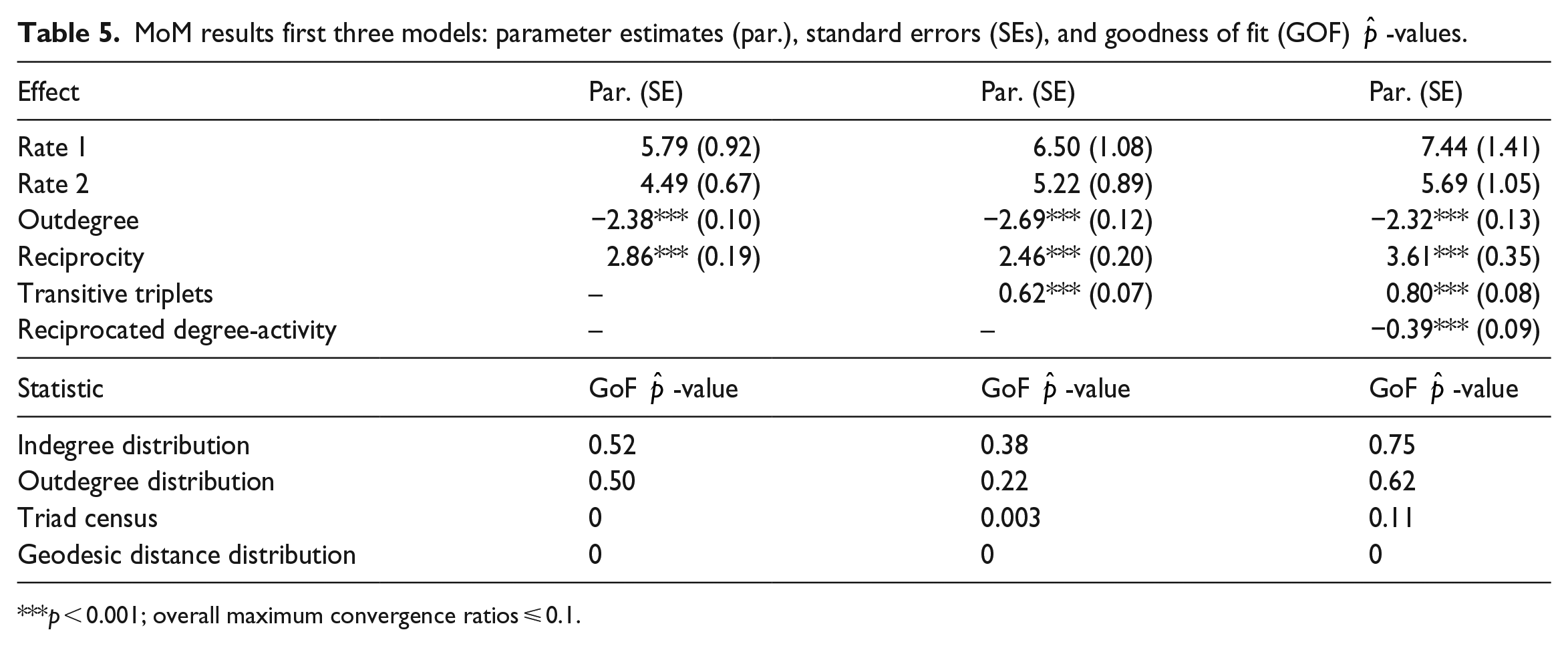
p < 0.001; overall maximum convergence ratios ⩽ 0.1.
MoM results last three models: parameter estimates (par.), standard errors (SEs), and goodness of fit (GOF)
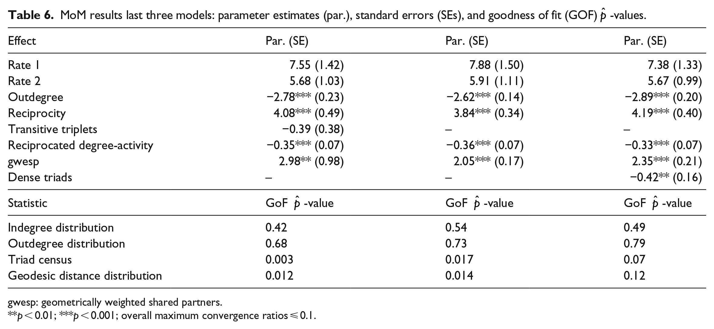
gwesp: geometrically weighted shared partners.
p < 0.01; ***p < 0.001; overall maximum convergence ratios ⩽ 0.1.
In view of the length of this article, we present only few plots. Figure 4 is a plot for the GOF results for the first model, containing only the outdegree and reciprocity effects, for the geodesic distance distribution of the auxiliary statistic. The fit is clearly very poor, with
In the first two steps the critical statistic was the triad census, and the effects added were transitive triplets and reciprocated degree-activity. In the third step the critical statistic was the geodesic distance distribution, and the gwesp effect was added. This led to an unforeseen result: the transitive triplets effect, included earlier, became insignificant. Also, the triad census GoF
For the final model, a plot for the GOF results is in Figure 5. For the visual comparison of Figures 4 and 5, keep in mind that the observed values are the same, and the simulated distributions now are much closer to the observations.
Discussion
This article proposed a GOF testing procedure for SAOMs which relies on a battery of auxiliary statistics, selected by the researcher, as GOF criteria. These statistics are used to construct a Monte Carlo Mahalanobis distance based test. Because remediating poor fit on these statistics can be a complex and time-consuming undertaking, we proposed the MMD estimator for the Mahalanobis distance, evaluated at some provisional model, to assess which model among a set of candidates can be expected to improve fit best.
The techniques proposed in this article can be directly extended to more elaborate SAOMs, for example, to studies of networks and behavior (Steglich et al., 2010).
The GOF test proposed and applied in this article, and the example data set, are freely available in the R package RSiena through the sienaGOF function. For more information on RSiena, the reader is referred to its homepage at http://www.stats.ox.ac.uk/snijders/siena/. Scripts using this function, complete with annotations, are available from the homepage.
Footnotes
Appendix 1
For the derivation of (17a), we begin with the i th coordinate of the derivative
Use the chain rule to obtain
Noting that
Denote
The middle term requires some more work. Since
where we have denoted
Putting these together, we obtain
Acknowledgements
We are grateful to Marijtje van Duijn and Nynke Niezink for their helpful comments on an earlier draft.
Declaration of conflicting interests
The author(s) declared no potential conflicts of interest with respect to the research, authorship, and/or publication of this article.
Funding
Most of the research for this article was conducted while the first author was a Rhodes scholar and the second author was employed by the University of Oxford. The authors received no further financial support for the research, authorship, and/or publication of this article.