Sage Journals: Discover world-class research

Abstract

Initially proposed by Marcoulides and further expanded by Raykov and Marcoulides, a structural equation modeling approach can be used in generalizability theory estimation. This article examines the utility of incorporating auxiliary variables into the structural equation modeling approach when missing data is present. In particular, the authors assert that by adapting a saturated correlates model strategy to structural equation modeling generalizability theory models, one can reduce any biased effects caused by missingness. Traditional approaches such as an analysis of variance do not possess such a feature. This article provides detailed instructions for adding auxiliary variables into a structural equation modeling generalizability theory model, demonstrates the corresponding benefits of bias reduction in generalizability coefficient estimate via simulations, and discusses issues relevant to the proposed approach.

Keywords

Auxiliary variables factor analysis generalizability theory missing data structural equation modeling

Generalizability theory

When it comes to educational and psychological measurements, the estimate of reliability—an index reflecting the precision of an assessment—provides the researcher with a critical understanding of measurement quality. For example, when attempting to determine an individual’s mathematical proficiency, it is common to use a set of relevant test items (items) to gauge proficiency. However, according to measurement theory, the measurement process itself can be rife with multiple, simultaneously occurring measurement errors. Indeed, the raw test scores within such a scenario are implicitly distinct from the phenomenon being measured and, therefore, cannot accurately reflect the true skill level of an examinee. By controlling for various measurement errors, statistical frameworks, such as the well-known classical test theory (CTT), yield more accurate estimations of proficiency or skill level. Within this context, measurement reliability is expressed as the correlation between the true skill levels of an examinee and those observed levels of skill represented by a testing score.

Within the framework of CTT, which assumes (1) each observed score has errors and (2) the errors follow a normal distribution, an observed score is equal to a true score plus the measurement error (i.e. X = T + e). Here coefficient α provides the mathematical equivalent of parallel tests, allowing for a derivation of test reliability that indicates what proportion of observed test score variance is attributable to true score variance (Cronbach, 1951). However, as this approach only assumes two components for a test score (i.e. true score and measurement error), this technique promotes an overly simplistic solution within the context of most research designs. To overcome this shortcoming, CTT and Cronbach’s alpha have been further extended to generalizability theory (G theory) (Cronbach et al., 1972).

While CTT calls for the decomposition of observed variances into true score variance and a single, all-compassing error term, G theory allows the researcher to account for several sources of variation, also known as facets. This provides for the disentanglement of any number of sources of measurement error originating from test items and/or graders. Such robust control of measurement error is simply not possible with CTT, and is what allows G theory to attain greater accuracy when generalizing observed scores to a broader universe.

G theory can provide the variance estimates for a wider variety of errors than CTT—errors that should not be ignored in a research design. These variance estimates allow one to calculate the level of generalizability or dependability of behavioral measurements. While research designs focused on generalizability are used to examine relative interpretations of measurement outcomes, those which aim at dependability are applied toward absolute interpretations. G theory decomposition also enables researchers to make decisions about how to increase generalizability/dependability coefficient to any specified level. For example, if one uses G theory and finds that there is large variance in grader effect (i.e. a lack of consistency among graders, which is undesirable), a follow-up G theory study (namely, a decision study, or D-study) can be used to identify the number of graders required for the measurement to reach a sufficient level of precision.

G theory provides answers to questions such as the following: What is the largest source of error? Is the study generalizable enough to provide important insights regarding latent variables of interest? Based on the current analysis, what test alterations can be made to reach a certain level of generalizability/dependability? These features provide G theory with wide applicability within the realm of psychological and educational assessments. For instance, Dunbar et al. (1991) studied the generalizability of findings across a substantial number of direct writing assessments, Gebril (2009) applied G theory in language testing, Jiang and Raymond (2018) used G theory to investigate subscore validity in score reporting, and Raymond, Clauser, and van Zanten (2009) studied spoken English proficiency scores within a G theory framework. Essentially, selecting an appropriate modeling strategy for a G theory study depends on the research designs. Nested design is a research design where levels of one facet are hierarchically subsumed under or nested within levels of another facet. Crossed design is a research design that has at least two facets that are crossed, that is, every category of one facet co-occurs in the design with every category of the other facet. Here a facet is defined by a certain set of conditions.

In a testing context, for example, test items and test administrations could be regarded as two separate facets. However, a test-taker’s ability is the object of measurement (Nuβbaum, 1984). Here, an educational testing scenario, which incorporates test-takers, items, and test-raters (raters), is used for illustration. Setting rater effect aside for the moment, the mathematical expressions for a typical one-facet, fully crossed design are as follows

X_{p i} = μ + μ_{p} + μ_{i} + μ_{p i}

(1)

σ {(X)}_{p i}^{2} = σ_{p}^{2} + σ_{i}^{2} + σ_{p i . e}^{2}

(2)

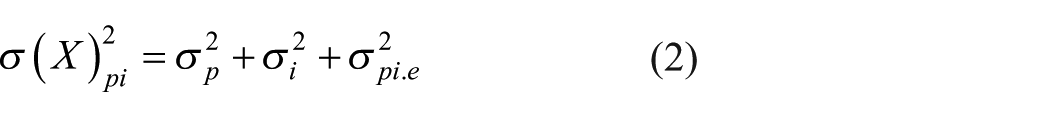
Equation (1) shows that an observed score, X, for person p on item i is defined by the sum of the grand mean µ, person effect µ_p, item effect µ_i, and error effect µ_pi. Note that the fully crossed design in the current scenario means that all persons have responded to all items. Correspondingly, the relevant variance components are outlined in equation (2). A typical two-facet, fully-crossed design can be expressed as follows

X_{p j i} = μ + μ_{p} + μ_{i} + μ_{j} + μ_{p i} + μ_{i j} + μ_{p j} + μ_{p j i}

(3)

σ {(X)}_{p j i}^{2} = σ_{p}^{2} + σ_{i}^{2} + σ_{j}^{2} + σ_{p i}^{2} + σ_{i j}^{2} + σ_{p j}^{2} + σ_{p j i . e}^{2}

(4)

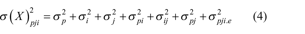
In addition to person effect µ _p and item effect µ _i , equation (3) also contains rater effect µ _j as well as interaction terms for any two random components. Equation (4) provides variance components in accordance with equation (3). In both one- and two-facet designs, all $σ s$ are dispersion parameters from independent and identically distributed (iid) normal shapes whose central locations are all equal to zero. Similarly, the fully crossed design in here means that all persons have responded to all items which are graded by all raters.

After estimating variance components, the G coefficient, a reliability-type index, can be calculated. As the aforementioned delineation between generalizability and dependability implies, the G coefficient can be either relative (norm-referenced) or absolute (criterion- or domain-referenced) (see Brennan, 1997, for details). However, here, only the norm-referenced G coefficient is addressed. The G coefficient, based on relative errors, is defined as follows

E ρ_{δ}^{2} = \frac{σ_{p}^{2}}{σ_{p}^{2} + σ_{δ}^{2}}

(5)

$σ_{δ}^{2}$ is a relative error variance term, which can be expressed as follows

σ_{δ}^{2} = \frac{σ_{p i}^{2}}{n_{i}} + \frac{σ_{p j}^{2}}{n_{j}} + \frac{σ_{p j i . e}^{2}}{n_{i} * n_{j}}

(6)

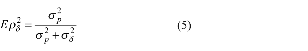
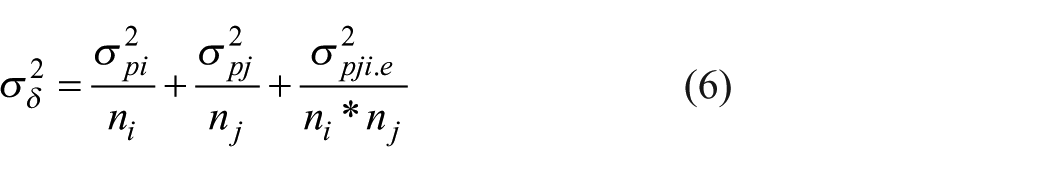
for a design that is defined by equations (3) and (4), where $n_{i}$ and $n_{j}$ are the numbers of levels for µ _i and µ _j effects, respectively. This article focuses on the impact of missing data on G coefficient. In addition, an approach based upon structural equation modeling is proposed to handle the problem.

Structural equation modeling (SEM) approach in G theory

SEM is widely used in the psychological, educational, and behavioral sciences. It is a powerful technique combining multivariate observed variables with complex structures. For instance, Figure 1 shows a simplified SEM example for modeling life satisfaction, turnover intent, and organizational citizenship behavior that are linked with 12 manifest or observed variables. Here, all three latent variables are measured with statement-based, self-report instruments and a Likert-type scale (see Schreiber, 2008). Note that a manifest analysis model differs from the latent models in the variables included: unlike latent models such as SEM, the manifest analysis model only contains observed variables and does not have any latent variable.

Figure 1.

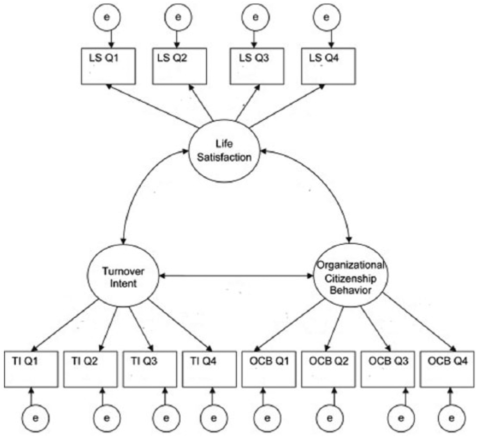
A structural equation model example for life satisfaction, turnover intent, and organizational citizenship behavior.

Within a SEM framework, one can verify the relations between (1) observed variables and latent/unobservable variables and (2) any pair of latent/unobservable variables. In the case of Figure 1, SEM allows the researcher to investigate the ways in which latent variables correlate with one another. In addition to providing insights linked to causal inferences and path analyses, SEM can also be used to study those longitudinal/repeated measurements typical to growth modeling and path analysis.

Within the context outlined here, G theory estimations are based primarily upon a special case of SEM known as confirmatory factor analysis (Jöreskog, 1969), which provides several benefits not present with other methods. For instance, the SEM approach can derive model fit indices, calculate standard errors of the estimates, and handle missing data. It is likely that such benefits have led to an increased use of SEM over the past decade by researchers like Gessaroli and Folske (2002), Hagtvet (1997, 1998) Marcoulides (1996, 2000) and Raykov and Marcoulides (2006).

Marcoulides (1996) described how to derive estimations using G theory within the context of a covariance structure analysis, while Raykov and Marcoulides (2006) fit this methodology within the SEM framework. Here a brief introduction to these methods is provided. Consider a two-facet, fully crossed design where the number of test-takers, items, and raters are 100, 5, and 2. Following the structure and notations of Raykov and Marcoulides, a corresponding diagram is presented in Figure 2. Rectangular boxes containing the letter Y represent observed variables, whose subscripts indicate their respective groupings. For example, Y32 contains the responses for the 100 test-takers to Item 3 scored by Rater 2. Latent variables—the variance components of G theory—are represented by circles. µ _p represents person effect. µ _pi ¹ to µ _pi ⁵, constrained to be equal, represent the interactions between item and person effects. The same applies to µ _pr ₁ and µ _pr ₂ so that the interaction between rater and person effects can be derived. Each arrow is a factor loading that regresses a certain variance component on a corresponding observed variable Y. These loadings are equal to one (1). Note, not all residuals for observed variables are shown in Figure 2. Nevertheless, they are constrained to be equal when a computation is performed. Mathematical proofs of converting a G theory model to SEM can be found in Raykov and Marcoulides (2006). With the rapid development of various statistical software packages, standard errors of estimates in SEM are now computed more easily than many other solutions, such as a traditional analysis of variance (ANOVA) (Searle, 1971) or restricted maximum likelihood (REML) estimator (Shavelson and Webb, 1991).

Figure 2.

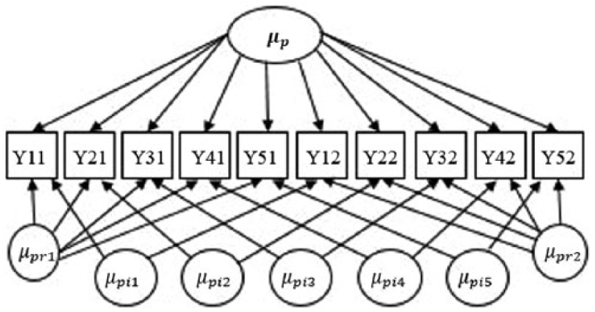
A structural equation model for estimating the variance components in a two-facet fully crossed design.

Missing data in SEM framework

A majority of scholars outside of the field applied statistics remain blissfully unaware of the dangers of missing data. They are unaware of techniques that could help nullify the negative effects of missing data within their research studies. Indeed, previous research has shown how cases of pairwise and case-wise deletion hurt validity—and yet the use of data flawed in this manner persists. What’s more, in the face of missing data, the use of inappropriate methods continues to inform biased estimates that lead to invalid conclusions (Enders, 2008). For these reasons, it is of the utmost importance that researchers become familiar with those statistical techniques that provide a robust solution to the problem of missing data.

There are three types of missing data. Data can be missing completely at random (MCAR), missing at random (MAR), or not missing at random (MNAR) (Little and Rubin, 2002). With data that are MCAR, missingness is defined independently of other observable and missing data. For example, a questionnaire/survey might be lost in the post, or a web browser malfunction might lead to the loss of question response records. In the case of data that are MAR, missingness is defined independently of missing data themselves, given other observed data. Furthermore, once those observed data are controlled for, missingness is explainable independently of any missing data. For example, if test data are missing due to test-taker illness (i.e. the test-taker was not present to provide data), the missingness is sufficiently explainable by the test-taker’s circumstance and has no relation to those data that would have been provided had the test-taker not fallen ill. Finally, missingness of data said to be MNAR is attributable to unobserved data (Allison, 2001; Enders, 2010). For example, a person does not complete a drug screening because they have used drugs and do not want to fail the test (Kang, 2013). Importantly, while solutions are available to account for missing data in the cases of MCAR and MAR, there are no appropriate solutions to MNAR.

To reiterate, the MAR assumption holds when the probability of missing data for a particular variable relates to other variables (informative variables) present in the model. If the informative variables are not included in the model, the analysis is performed with an MNAR mechanism, which tends to produce biased estimates. Therefore, MAR and MNAR differ in their inclusion of informative variables within a given model. In the current article, only MAR is considered because (1) true MCAR is rare in practice and (2) the solutions that work for MAR mechanism also works for MCAR situations. Particular in G theory literature, missing issues are discussed intensively within a MCAR pattern, which is essentially treated as unbalanced data situation. For example, Brennan (2001) used analogous-ANOVA estimators, also known as Henderson’s (1953) Methods 1 and 3, to adjust unequal sample sizes in different groups. In yet another example, Chiu and Wolfe (2002) proposed subdividing method by “creating data sets that exhibit structural designs that are common in generalizability analyses.”

Recent missing data studies have demonstrated advantages of an “inclusive analytic strategy” that incorporates auxiliary variables into the analysis model or into the imputation process (Enders, 2008). An auxiliary variable is defined as a variable that one would include in an analysis because it provides the information about the part of data that are missing (Collins et al., 2001; Rubin, 1976; Schafer, 1997; Schafer and Graham, 2002). As described previously, to meet the MAR assumption, the “cause” information must be considered when data are modeled. Indeed, this “cause” information defines those auxiliary variables, the primary function of which is to reduce potential bias within any explanatory model—as opposed to providing direct explanatory insights of those phenomena being studied.

Many studies have illustrated how auxiliary variables can be used to bolster explanatory power and mitigate bias by recapturing certain lost information (Collins et al., 2001; Enders, 2008). Nevertheless, such methods are not fool proof, in that they cannot guarantee unbiased estimates (Enders, 2010). Instead, success depends upon how well auxiliary variables correlate with missingness or any incomplete variables within the model under study—as signaled by the degree of bias reduction in model estimations. To illustrate, if income is an important variable within a survey analysis, a question that asks respondents to report their occupation will likely provide a good auxiliary variable, due to the correlation between the resulting data and income.

Although auxiliary variables have fewer downside effects on a model’s parameter estimates, fitting a maximum likelihood estimation with a large number of auxiliary variables can be problematic, due to complex specification (Enders, 2010: 133). That said, to successfully perform a likelihood-based estimation, one should only incorporate auxiliary variables that have more informative utility. An ideal auxiliary variable can reflect, or at least highly correlate with, the true cause of missingness within a model. Selecting useful auxiliary variables, however, is not always a straightforward process. In many cases an extensive review of the pertinent literature may be called for, coupled with good, old-fashioned guesswork. For example, knowing that family mobility can lead to school attrition, a researcher conducting survey researcher might ask households to report the likelihood of an upcoming move (Enders et al., 2006; Graham et al., 1997). In addition to utilizing theory to guide one’s selection of appropriate auxiliary variables, statistical evidence may also be used. Collins et al. (2001) any variable that correlating at a level of 0.4 or higher with any incomplete variable, would make for a good auxiliary variable.

Graham (2003) described two SEM-based strategies for incorporating auxiliary variables into a maximum likelihood analysis: the extra dependent variable model and the saturated correlates model. Here, the inclusion of auxiliary variables is possible without fear of altering the interpretation of substantive theoretical constructs of interest. The saturated correlates model, in particular, provides for an easier path than the extra dependent variable model, while producing similar results. Alternatively, researchers have proposed the various versions of a two-stage approach, while cautioning that inappropriate specification of auxiliary variables could lead to some bias (see Savalei and Bentler, 2007 and Yuan and Bentler, 2000 for details).

Given the reasons just cited, the authors propose the saturated correlates model as the preferred choice. The term “saturated” does not imply a full model (i.e. a model with a perfect fit). Instead, the name follows from the fact that the model includes all possible associations among the auxiliary variables as well as all possible associations between the auxiliary variables and the manifest analysis model variables (i.e. the auxiliary variable portion of the model is saturated). To be concrete about the saturated correlates model concept, the degrees of freedom of the model tested in Figure 3 is 51; that is to say, df = 78–27 because there are 12 × 13/2 = 78 unique elements in the observation variance/covariance matrix, and df consumptions are (1) four aforementioned random effects: $σ_{p}^{2}, σ_{p i}^{2}, σ_{p j}^{2}$ , and $σ_{p j i . e}^{2}$ , (2) 3 variance/covariance components of the auxiliary variables matrix, and finally, (3) the 10 loadings that each auxiliary variable on the response variables (therefore 10 × 2 = 20). Note, the loadings pointing from µ _p , µ _pr ₁, µ _pi ₁, µ _pi ₂, µ _pi ₃, µ _pi ₄, µ _pi ₅, µ _pr ₂ to all Ys are constrained to 1 and therefore need no estimation. Here it should be noted that the procedure for incorporating auxiliary variables in a manifest model versus a latent model differ slightly (see Graham, 2003, for the differences). In the case of latent models, as seen with SEM, one should incorporate correlating auxiliary variables with (1) observed predictors, (2) other auxiliary variables, and (3) the error variance of the observed indicators.

Figure 3.

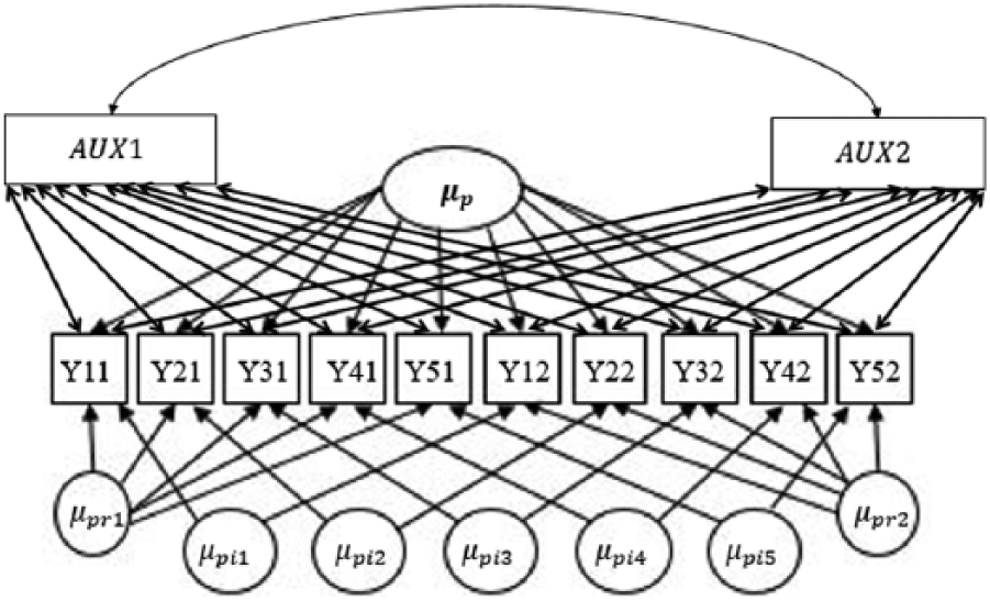
A saturated correlates model for estimating the variance components in a two-facet fully crossed design with missing data.

Yoo (2009) utilizes a Monte Carlo analysis to examine variable performance of auxiliary variables. Specifically, Yoo simulates responses from an eight-variable, two-factor measurement model and uses a six-variable, two-factor measurement model for evaluation, after excluding two auxiliary variables. By altering (1) the levels of factor loadings, (2) the correlations between auxiliary and latent variables, (3) the probability of missing, and (4) the missing mechanism, Yoo finds that including auxiliary variables in the confirmatory factor analysis (CFA) model can improve parameter estimation in most cases, particularly in cases of MAR data associated with the absence of auxiliary variables in the imputation model.

In this article, auxiliary variables are incorporated into the saturated correlates model, a SEM-based approach, to handle missing data problems in a G theory study. The research hypotheses are (1) MAR missing data can lead to biased G coefficient estimates to a degree in accordance with the variance size and the association with the missing cause(s), (2) using the proposed approach would yield more accurate estimates when missing data exist, and (3) it is a safe strategy to incorporate auxiliary variables into the model because it has no harmful impacts on the actual estimates even with no missingness. Figure 3 illustrates the application of G theory within a SEM framework. Aside from the inclusion of two auxiliary variables (AV1 and AV2), which correlate (1) with each other and (2) with the indicators’ error variance, this model is identical to that seen in Figure 2. In addition, bi-directional arrows represent correlations between auxiliary variables and observed variables. In the coming simulation section, synthetic data are all modeled following the same strategy.

Within this study, lavaan is used to conduct SEM analysis. As described by Rosseel (2012), lavaan is a software package for use within the R software environment. It is an open source software that provides a straightforward approach to constructing complex SEM frameworks. In the hope that it will provide a more approachable example of the concepts shared herein, Figure 4 illustrates the lavaan coding syntax used for constructing the theoretical model shown in Figure 3 (see link for downloading the script file). Within Figure 4, the first line of code displays HS.model, an object that contains a G theory SEM model that meets those parameters outlined in coding lines 2 through 30. Furthermore, facets such as person effect, item effect, and rater effect are represented by the coding variable labels p_factor, i_factor, and r_factor, respectively. Here also, ys represent indicators, while auxs represent auxiliary variables. Finally, pvar, ivar, and rvar represent functions used to constrain the equivalency of estimates within the model. The right-most portion of those formulas contained in coding lines 2 through 9 are predicted by corresponding facets shown to the left of the =~ symbol—where all loadings are set to 1. Coding lines 10 through 30 use ~~ to represent correlation (if linking different variables) and variance/residuals (if linking the same variable). For example, aux1 ~~ aux2 specifies the correlation between the two auxiliary variables, while coding lines 11 and 12 prompt correlation comparisons between each auxiliary variable and all other observed variables. At Lines 19 and 20, the variance of r_factor1 and the variance of r_factor2 are set to equal by rvar. The similar idea applies to other constraint labels such as pvar and res. Line 31 feeds the specified HS.model object to the lavaan function sem such that the model can be actually executed. Here also, the data set which contains missing data is named lav_dat. Furthermore, the method of deriving those missing data within this SEM model is set to full information maximum likelihood (FIML), and, finally, the exoxenous latent variables are assumed to be uncorrelated by setting the orthogonal model feature to TRUE. Additional details regarding SEM model specification within the lavaan R package can be found in Rosseel (2012).

Figure 4.

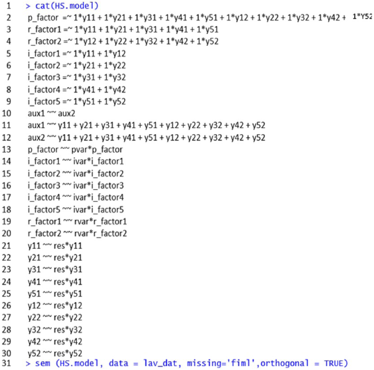
Lavaan specification for the model illustrated in Figure 3.

Simulation design

The process of testing the utility of a SEM framework began with a pilot study conducted using a data set that contained no missing values. The results of this pilot show that when data are complete, both SEM and REML yield extremely similar estimates. To investigate the utility of incorporating auxiliary variables into SEM G theory, a comprehensive simulation study was conducted. Instead of arbitrarily choosing variance component values, the results of the California Assessment Program (CAP) dependability analyzed by Shavelson et al. (1993) were used to serve as a baseline for data generation. For the purpose of notation consistency, the facet of measurement occasion is treated as an item facet. Here it should be noted that this type of two-item design is not uncommon within the realm of educational assessment, especially when such assessments are aimed at writing tasks.

Within the context of equations (3) and (4), outlined in an earlier section of this article, the baseline true parameters are $σ_{p}^{2} = 0.298$ , $σ_{i}^{2} = 0.092$ , $σ_{j}^{2} = 0.003$ , $σ_{p i}^{2} = 0.493$ , $σ_{p j}^{2} = 0.000$ , $σ_{i j}^{2} = 0.002$ , and $σ_{p j i . e}^{2} = 0.148$ . Correspondingly, the numbers of levels of µ _p , µ _i , and µ_j effects are $n_{p} = 50$ , $n_{i} = 2$ , and $n_{j} = 3$ respectively. Here a Monte Carlo sampling approach is used to simulate data responses. Furthermore, it should be noted that the CAP study was originally conducted under a two-facet, fully crossed design as exemplified within equations (3) and (4). The SEM approaches illustrated in Figures 2 and 3 formed the basis for data analysis.

In order to inject variance within the G coefficient during testing, three additional levels of person effect, $σ_{p^{'}}^{2} = (0.098, 0.698, 1.698)$ , were used. These levels, although somewhat arbitrary, are specified here for reference purposes. That is to say, these values were chosen to help to show how results vary, depending on the degree of person effect variance. Alternatively, manipulating G coefficient levels can be achieved by varying $n_{i}$ or/and $n_{j} .$ However, keeping simulation parameters consistent with this study’s purpose, variations were limited to the person effect (i.e. $σ_{p^{'}}^{2}) .$ To summarize, there were four levels of person effect utilized in this simulation design—the original effect when no data were missing, as well as the three variable effects designated when predicting values using incomplete data sets.

After generating responses from a given true variance set, incomplete data conforming to a MAR pattern were injected into the data. Following the approach prescribed by Park and Shin (1998), a MAR pattern was injected into the data set via two auxiliary variables (AV1 and AV2) derived by simulating two columns of data correlating with µp. Here it should be noted that the method for deriving AV1 and AV2 falls in line with that approach taken by Wu et al. (2015). In addition, three levels of average correlation were used to generate AV1 and AV2: $\bar{ρ_{a v . p}} = \pm 0.1, \pm 0.5, \pm 0.9$ . That is, for a specified level of $\bar{ρ_{a v . p}}$ , for example 0.9, the two actual correlations between auxiliary variables and person effect could take on the values $ρ_{a v 1 . p} = 0.95$ and $ρ_{a v 2 . p} = 0.85$ , or $ρ_{a v 1 . p} = 0.90$ and $ρ_{a v 2 . p} = 0.90$ .

Consistent with the modeling practice outlined in Figure 3, there were $n_{i} * n_{j}$ indicators in the primary model structure. Missing data for these indicators were incorporated into the data set based on AV1 and AV2. To be more specific, splitting the indicators evenly into two subsets, AV1 produced missing cells for the first subset and AV2 produced missing data for the second subset. The ordered AVs were ranked from smallest to the largest, while the probability of any particular data point being marked as missing was based on that datum’s rank order. As an example, for the first indicator, the probability of having missing data was computed as 1 minus the rank order of the value of $AV 1 / n_{p}$ . This probability is then compared to a random number drawn from a uniform distribution ranging from zero (0) to one (1). Where the probability is higher than the random draw, the corresponding cell is set as missing. This procedure continues for each indicator, barring one, until a pre-defined percentage of missing data is met. Here it should be noted, leaving one indicator intact prevents any change in the sample size that would nullify prescribed percentage levels of missingness assigned for each simulation. Furthermore, for the purposes of this study, percentage levels of missing data were set to 15%, 45%, and 75%.

Given that REML and the FIML produce nearly identical results within the context of large samples, a FIML estimator approach to SEM, as seen in the work of Raykov and Marcoulides (2006), is used here. In total, this FIML simulation study incorporates 72 conditions, each of which are replicated 500 times. Feinberg and Rubright (2016) suggest that performing simulation studies of this kind requires at least 250 times. Based on the results provided, the accuracy of G coefficient and its variance component estimates are examined. The bias and mean square error (MSE) of each estimate in all conditions were recorded. The formula to calculate absolute bias is

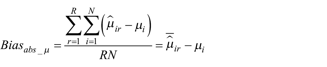
B i a s_{a b s_μ} = \frac{\sum_{r = 1}^{R} \sum_{i = 1}^{N} ({\hat{μ}}_{i r} - μ_{i})}{R N} = {\bar{\hat{μ}}}_{i r} - μ_{i}

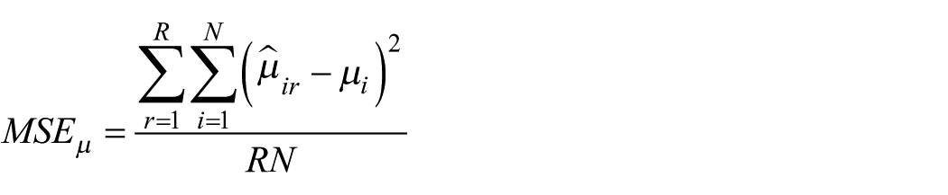
In order to make simulations comparable across different settings, relative bias, obtained by $B i a s_{θ} / θ_{i}$ , is used instead. From here the bias is referred as relative bias represented by a percentage number. MSE can be calculated by

M S E_{μ} = \frac{\sum_{r = 1}^{R} \sum_{i = 1}^{N} {({\hat{μ}}_{i r} - μ_{i})}^{2}}{R N}

Where N is the number of elements in the set of $θ$ and R is the number of replications. In addition, the standard errors provided via SEM analyses are examined. Using the standard errors of the estimates, one can construct confidence intervals for estimated variance components at a nominal $α$ level (e.g. 0.05). Since the lavaan package derives standard errors in a typical fashion, and the lower bound for these variance components is equal to zero, constructing confidence intervals requires data transformation: $\exp (1 n (\hat{μ}) \pm 1.96 * (1 n(sd(\hat{μ}))$ . As simulations progress, a coding element produces a binary indicator that signals when the standard error for data estimates surpass the set confidence interval.

Simulation results

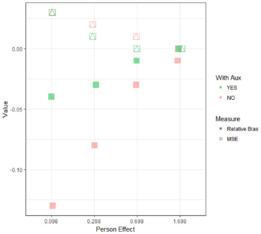
Comprehensive results for FIML simulations can be found in Appendix 1. In addition, Figure 5 shows the G coefficient bias and MSE results when the missing percentage is set to 15%. When $σ_{p}^{2}$ is smaller (i.e. a smaller, true G coefficient), the relative bias and MSE tended to be larger. To illustrate, given that the estimation was No Aux and $\bar{ρ_{a v . p}}$ was equal to −0.9, the relative bias for G coefficient was −25.66%, when $σ_{p}^{2}$ was equal to 0.098 which resulted in a true G coefficient equaled to 0.265. The relative bias reduced to −2.20% when $σ_{p}^{2}$ increased to 1.698 while holding other controlled variables constant.

Figure 5.

Average relative biases and mean square errors across six correlation levels.

For a given absolute value of $\bar{ρ_{a v . p}}$ , both negative and positive values tended to produce similar relative bias and MSE estimates. With Aux yielded more accurate G coefficients in 17 out of 24 conditions; the seven exceptions, however, showed that the corresponding biases produced by With Aux and No Aux were extremely close. A similar trend can be found in the MSE result panel. Therefore, it can be concluded that With Aux outperforms No Aux in terms of both estimate accuracy and efficiency. As one might expect, when the absolute value of $\bar{ρ_{a v . p}}$ is small, With Aux did not improve the estimate accuracy, whereas a larger absolute value of $\bar{ρ_{a v . p}}$ led to improved accuracy in the With Aux model. For instance, when $σ_{p}^{2}$ was 0.698, With Aux reduces the G coefficient relative bias from −6.67% to −0.56% at the condition that $\bar{ρ_{a v . p}} = 0.9$ , where the reduction became 1.39% (i.e. 3.06%–1.67%) at $\bar{ρ_{a v . p}} = 0.5$ condition.

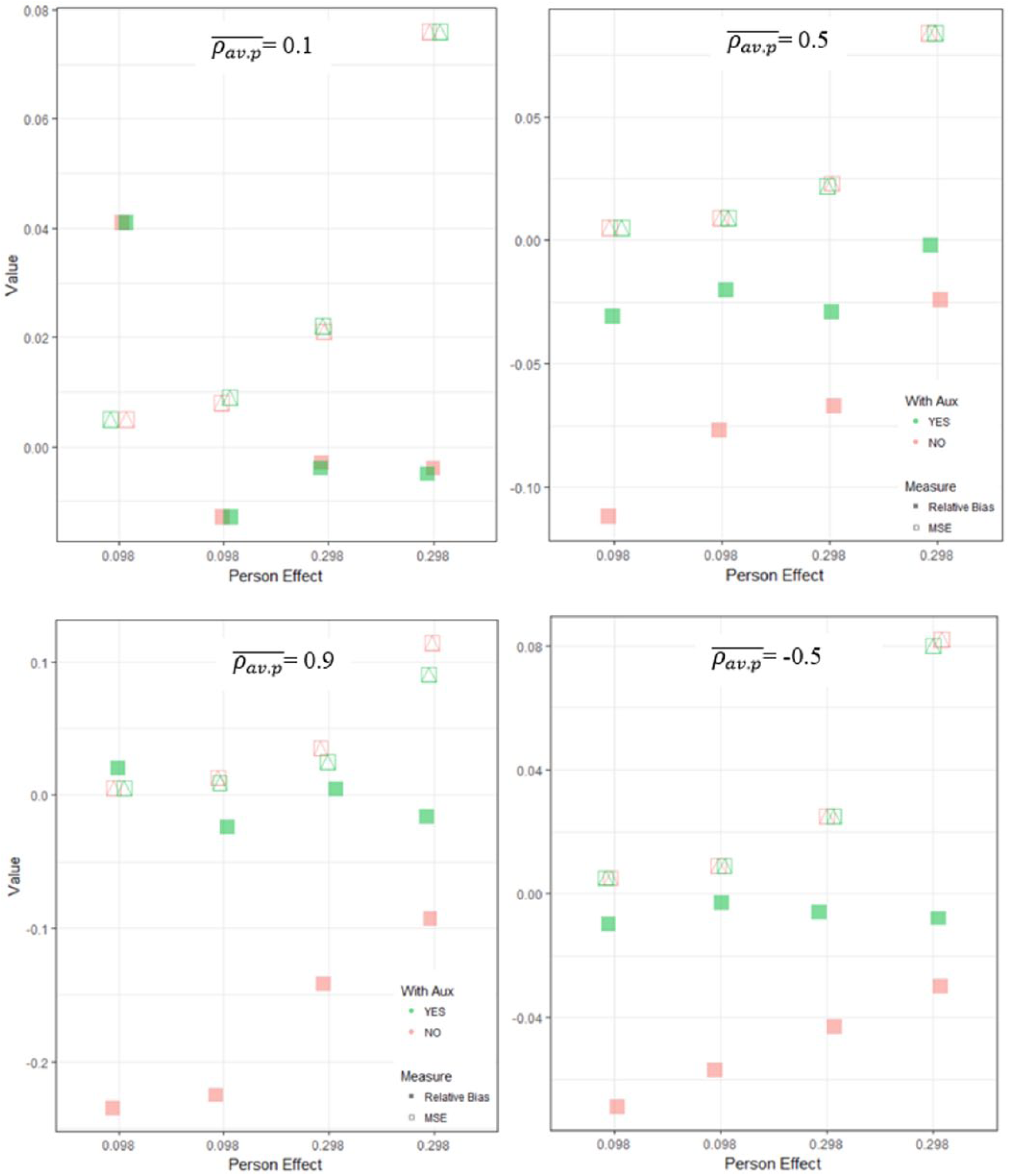
To analyze how the components of G coefficients function within this simulation study, the biases and MSEs of $σ_{p}^{2},$ $σ_{p i}^{2}$ , $σ_{p r}^{2}$ , and $σ_{p j i . e}^{2}$ are examined. Figure 6 lists the relative biases and MSEs of $σ_{p}^{2}$ under conditions of 15% missingness. As one can see, With Aux simulations recovered the $σ_{p}^{2}$ estimates with greater accuracy and efficiency than seen with No Aux simulations. For a given absolute value of $\bar{ρ_{a v . p}}$ , being negative or positive did not change the estimates provided by both modeling strategies. When the absolute value of $\bar{ρ_{a v . p}}$ increased, No Aux tended toward greater bias and inefficiency. At the same time, within those same conditions, the capacity of With Aux simulations to correct for imprecise estimates strengthened. These patterns are similar to those illustrated within Figure 5.

Figure 6.

Sample average relative biases and mean square errors for $σ_{p}^{2}$ estimates.

Here it should be noted that the MSE of $σ_{p}^{2}$ is consistently smaller than the corresponding G coefficient. Furthermore, although $σ_{p i}^{2}$ is not the cause of the missing data, in several circumstances the estimates are noticeably biased. For example, when true $σ_{p}^{2}$ is 0.698 and $\bar{ρ_{a v . p}} = 0.9,$ the biases for No Aux and With Aux are 3.25% and −1.22% respectively. Similar to the $σ_{p}^{2}$ outcomes, MSE results show that, across all conditions, both modeling strategies provided highly efficient estimates. The other two components ( $σ_{p r}^{2}$ and $σ_{p j i . e}^{2}$ ) were not affected by missingness. Indeed, within the context of both estimations, their biases and MSEs all fall below 0.005 (many of them were below 0.001). Note, if true $σ_{p r}^{2}$ were to be set to a non-zero number, it would have been expected to produce bias and estimates similar to that seen with $σ_{p i}^{2}$ .

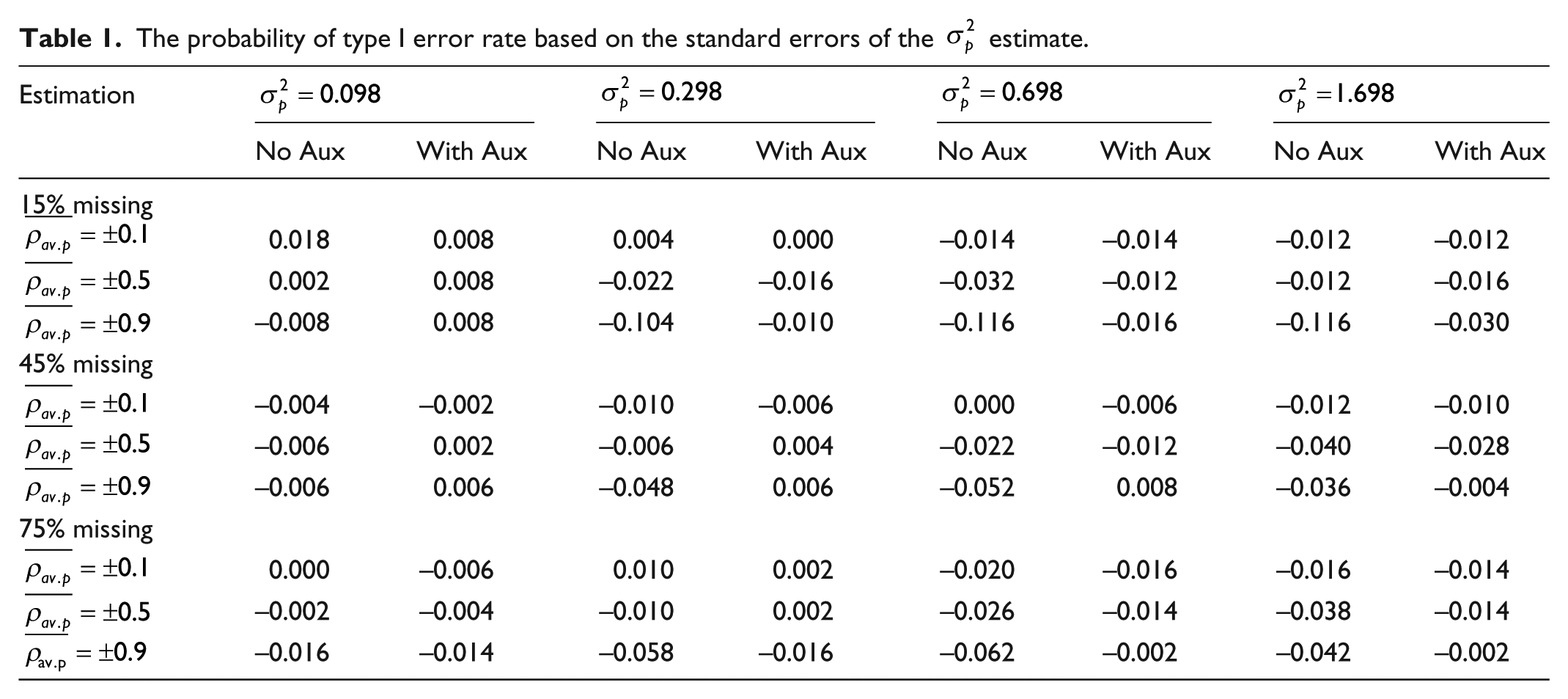
While the primary focus of this article is determining the accuracy of G coefficient estimates, standard errors of the estimates are also studied—since they speak to the quality of statistical inferences. As shown in Table 1, results of the true $σ_{p}^{2}$ coverage deviate up to 0.95 when using the standard errors of the estimate. Since the direction of $\bar{ρ_{a v . p}}$ yielded negligible differences in the current output, they were collapsed based upon their absolute values. Here, a negative value shows that the corresponding standard error is underestimated, while a positive value indicates overestimation. In both cases, such output indicates that Type I errors are not being effectively controlled for. What’s more, as the percentage of missingness increases, the level at which standard errors deviate from our set confidence interval increases. Cases of a larger absolute value of $\bar{ρ_{a v . p}}$ tended to result in less accurate standard error estimates. Compared with No Aux, which produced unstable standard errors across the simulation conditions, With Aux provided more accurate estimates—as even the largest coverage rate deviation from 0.95 was as low as −0.028. Nevertheless, the standard errors of other variance components are fairly good, considering that all deviations fall below 0.03 for both modeling approaches.

Table 1.

The probability of type I error rate based on the standard errors of the $σ_{p}^{2}$ estimate.

Estimation					$σ_{p}^{2} = 0.698$		$σ_{p}^{2} = 1.698$
	No Aux	With Aux	No Aux	With Aux	No Aux	With Aux	No Aux	With Aux
15% missing
$\bar{ρ_{a v . p}} = \pm 0.1$	0.018	0.008	0.004	0.000	–0.014	–0.014	–0.012	–0.012
$\bar{ρ_{a v . p}} = \pm 0.5$	0.002	0.008	–0.022	–0.016	–0.032	–0.012	–0.012	–0.016
$\bar{ρ_{a v . p}} = \pm 0.9$	–0.008	0.008	–0.104	–0.010	–0.116	–0.016	–0.116	–0.030
45% missing
$\bar{ρ_{a v . p}} = \pm 0.1$	–0.004	–0.002	–0.010	–0.006	0.000	–0.006	–0.012	–0.010
$\bar{ρ_{a v . p}} = \pm 0.5$	–0.006	0.002	–0.006	0.004	–0.022	–0.012	–0.040	–0.028
$\bar{ρ_{a v . p}} = \pm 0.9$	–0.006	0.006	–0.048	0.006	–0.052	0.008	–0.036	–0.004
75% missing
$\bar{ρ_{a v . p}} = \pm 0.1$	0.000	–0.006	0.010	0.002	–0.020	–0.016	–0.016	–0.014
$\bar{ρ_{a v . p}} = \pm 0.5$	–0.002	–0.004	–0.010	0.002	–0.026	–0.014	–0.038	–0.014
$\bar{ρ_{a v . p}} = \pm 0.9$	–0.016	–0.014	–0.058	–0.016	–0.062	–0.002	–0.042	–0.002

Discussion

Missing data can lead to biased estimates, and thus eliminating or reducing the influence of missing data is important when G theory analysis is used for decision making, especially those that are high stakes. It can be calculated from Table 1, in the condition where $\bar{ρ_{a v . p}} = 0.9$ and $σ_{p}^{2} = 0.698,$ the true G coefficient is 0.720 and the estimate can be as low as 0.676 if the auxiliary variables are not taken into account. If 0.7 is used as a criterion for an assessment quality evaluation, the biased G coefficient estimate, due to missingness, would lead to a conclusion that the assessment is not reliable enough. This finding indicates that when missingness occurs in a G theory study, one can find variables related to the study such that these variables can be incorporated into a SEM framework for more accurate G coefficient estimates. In practice, these variables can be demographic information such as ethnicity, incomes, education level, and ages. That said, one can extract information from different databases to achieve auxiliary variables. What is more, although preferred to highly correlate to the actual missing causes, these variables do not significantly alter G coefficient when they are not highly informative; it is a relatively safe strategy for modeling with low-quality auxiliary variables. To shed the light on the application of the proposed method, a recent study using “symptom-check-list-27-plus” (SCL-27-plus) along with the scale of the quality of life (QOL) is delineated here. Hardt et al. (2012) investigate symptoms of depression, agoraphobia, social anxiety, pain, and vegetative symptoms via the SCL-27-plus where the database involved missing cells that are susceptibly yielding an inaccurate analysis. In order to reduce the estimate biases, Hardt, Herke, and Leohart use QOL responses to serve as auxiliary variables by matching the identifications of respondents and the results show that the estimates are less biased when the QOL responses are aligned with the SCL-27-plus. Despite the fact Hardt, Herke, and Leohart’s study is not based upon G-theory, the idea of applying auxiliary variables to trade more accurate estimates is identical to that of the present article: when conduct a G-theory study, it is preferable for researchers to collect information from multiple resources, even some of the information is not the focus of research interest, such that the negative consequences of missing data can be minimized.

To keep simulation design manageable, the missing data mechanism was based upon person effect only. Although theoretically, it could relate to item effect and/or rater effect, in practice it is more viable to assume participants themselves are the missingness reason. Besides, in some situations, it would be redundant to assume that the causes of missing data stem from various effects simultaneously. To illustrate, participants from a high-income family are likely to miss a survey question about free and reduced lunch. Assuming that the missingness takes place due to the item being too difficult for persons from a high-income family, is in fact, commensurate with the assumption on persons’ socioeconomic statuses. This practice, correlating auxiliary variables with person effect only, would be attenuated when missing cells are removed from the full data set. That said, the actual correlation between missingness in an observed data set and an auxiliary variable is lower than what it would be at the person effect level.

Providing model fit is another important feature of SEM. In particular, if a G theory framework fits data poorly, further analyses based on the estimation will be untrustworthy. Essentially, G theory is a modeling framework like any other statistical models. Traditional estimations do not provide fit information about a certain G theory framework used in research; if a data set that was planned in a two-facet design but is inappropriately/wrongfully fitted into a one-facet design, the model fit in SEM is expected to capture the misfit. In addition, SEM has assembled with a FIML estimator, which makes the modeling easier for handling missing data problems without complicated corrective procedures (Allison, 2000). Recent model fit interpretation can be found in Kline (2015), Shi et al. (2017) and Shi et al. (2018).

Theoretically, SEM approach can estimate other main effects such as item effect and rater effect; it needs to handle the data format differently. For example, if one is interested in estimating the item effect, each row of the input data should be responses of an item (instead of a person). Practically, however, this practice often is not permissible as the levels of other main effects are not sufficiently large, while the person effect can result in many indicators. To solve the problem, Marcoulides (2000) derived an approach of estimating other main effects by analyzing the matrix of correlations. In this article, if a measurement is domain-referenced, SEM approach used here is not appropriate as it provides insufficient information. If absolute errors are needed and current existing software packages are considered, the saturated correlates model can be used to cross-validate the feasibility of the traditional approaches such as REML. If the common variance components from both estimations are close to a certain acceptable level, the effects that the saturated correlates model does not estimate can be obtained from REML. Alternatively, one can use a Bayesian framework to analyze a G theory study (Little and Rubin, 2014). During the Bayesian estimation process, missing data imputation can be accommodated simultaneously (Jiang and Skorupski, 2017; Qin, 2018).

Footnotes

Appendix 1 Declaration of conflicting interests

The author(s) declared no potential conflicts of interest with respect to the research, authorship, and/or publication of this article.

Funding

The author(s) received no financial support for the research, authorship, and/or publication of this article.

ORCID iD

Zhehan Jiang

Author biographies

Zhehan Jiang is an assistant professor at the University of Alabama, where his research interest is about psychometrics modeling and computations.

Kevin Walker is an associate professor at the University of Alabama, where he directs the assessment department at the libraries.

Dexin Shi is an assistant professor at University of South Carolina, where his works lies at structural equation modelings and model fits.

Jian Cao is a research assistant of High Performance Computing Center at Weifang University, where he is also a visiting scholar at the University of Queensland.

References

Allison

(2000) Multiple imputation for missing data: A cautionary tale. Sociological Methods & Research 28(3): 301–309.

Allison

(2001) Missing Data. Thousand Oaks, CA: SAGE.

Brennan

(1997) A perspective on the history of generalizability theory. Educational Measurement: Issues and Practice 16(4): 14–20.

Brennan

(2001) Generalizability Theory. New York: Springer.

Chiu

Wolfe

(2002) A method for analyzing sparse data matrices in the generalizability theory framework. Applied Psychological Measurement 26(3): 321–338.

Collins

Schafer

Kam

C-H

(2001) A comparison of inclusive and restrictive strategies in modern missing data procedures. Psychological Methods 6: 330–351.

Cronbach

(1951) Coefficient alpha and the internal structure of tests. Psychometrika 16: 297–334.

Cronbach

Gleser

Nanda

et al . (1972) The Dependability of Behavioral Measurements: Theory of Generalizability for Scores and Profiles. New York: Wiley.

Dunbar

Koretz

Hoover

(1991) Quality control in the development and use of performance assessments. Applied Measurement in Education 4(4): 289–303.

10.

Enders

(2008) A note on the use of missing auxiliary variables in full information maximum likelihood-based structural equation models. Structural Equation Modeling 15(3): 434–448.

11.

Enders

(2010) Applied Missing Data Analysis. New York: Guilford Press.

12.

Enders

Dietz

Montague

et al . (2006) Modern alternatives for dealing with missing data in special education research. in: Scruggs

Mastropieri

(eds) Applications of Research Methodology. Bingley: Emerald Group Publishing, pp. 101–129.

13.

Feinberg

Rubright

(2016) Conducting simulation studies in psychometrics. Educational Measurement: Issues and Practice 35(2): 36–49.

14.

Gebril

(2009) Score generalizability of academic writing tasks: Does one test method fit it all? Language Testing 26(4): 507–531.

15.

Gessaroli

Folske

(2002) Generalizing the reliability of tests comprised of testlets. International Journal of Testing 2: 277–295.

16.

Graham

(2003) Adding missing-data-relevant variables to FIML-based structural equation models. Structural Equation Modeling 10(1): 80–100.

17.

Graham

Hofer

Donaldson

et al . (1997) Analysis with missing data in prevention research. The Science of Prevention: Methodological Advances from Alcohol and Substance Abuse Research 1: 325–366.

18.

Hagtvet

(1997) The function of indicators and errors in construct measures: An application of generalizability theory. Journal of Vocational Education Research 22(4): 247–266.

19.

Hagtvet

(1998) Assessment of latent constructs: A joint application of generalizability theory and covariance structure modelling with an emphasis on inference and structure. Scandinavian Journal of Educational Research 42: 41–63.

20.

Hardt

Herke

Leonhart

(2012) Auxiliary variables in multiple imputation in regression with missing X: A warning against including too many in small sample research. BMC Medical Research Methodology 12(1): 184.

21.

Henderson

(1953) Estimation of variance and covariance components. Biometrics 9(2): 226–252.

22.

Jiang

Raymond

(2018) The use of multivariate generalizability theory to evaluate the quality of subscores. Applied Psychological Measurement. Epub ahead of print 3 April. DOI: 10.1177/0146621618758698.

23.

Jiang

Skorupski

(2017) A Bayesian approach to estimating variance components within a multivariate generalizability theory framework. Behavior Research Methods. Epub ahead of print 12 December. DOI: 10.3758/s13428-017-0986-3.

24.

Jöreskog

(1969) Efficient estimation in image factor analysis. Psychometrika 34(1): 51–75.

25.

Kang

(2013) The prevention and handling of the missing data. Korean Journal of Anesthesiology 64(5): 402–406.

26.

Kline

(2015) Principles and Practice of Structural Equation Modeling. New York: Guilford Press.

27.

Little

Rubin

(2002) Bayes and multiple imputation. Statistical Analysis with Missing Data 200–220.

28.

Little

Rubin

(2014) Statistical Analysis with Missing Data. New York: Wiley.

29.

Marcoulides

(1996) Estimating variance components in generalizability theory: The covariance structure analysis approach. Structural Equation Modeling 3: 290–299.

30.

Marcoulides

(2000) Generalizability theory: Advancements and implementations. In: Proceedings of the 22nd language testing research colloquium, Vancouver, BC, Canada, 9 March.

31.

Nuβbaum

(1984) Multivariate generalizability theory in educational measurement: An empirical study. Applied Psychological Measurement 8: 219–230.

32.

Park

Shin

(1998) An algorithm for generating correlated random variables in a class of infinitely divisible distributions. Journal of Statistical Computation and Simulation 61(1–2): 127–139.

33.

Qin

(2018) Estimating nonlinear indirect effects in Bayesian semiparametric structural equation model. Multivariate Behavioral Research 53(1): 130–131.

34.

Raykov

Marcoulides

(2006) Estimation of generalizability coefficients via a structural equation modeling approach to scale reliability evaluation. International Journal of Testing 6: 81–95.

35.

Raymond

Clauser

van Zanten

(2009) Measurement precision of spoken English proficiency scores on the USMLE Step 2 Clinical Skills Examination. Academic Medicine 84(10): S83–S85.

36.

Rosseel

(2012) Lavaan: An R package for structural equation modeling. Journal of Statistical Software 48(2): 1–36.

37.

Rubin

(1976) Inference and missing data. Biometrika 63: 581–592.

38.

Savalei

Bentler

(2007) Structural Equation Modeling. In: Grover

Vriens

(eds) The Handbook of Marketing Research: Uses, Misuses, and Future Advances. Thousand Oaks, CA: Sage Publications, pp. 330–364.

39.

Schafer

(1997) Analysis of Incomplete Multivariate Data. New York: Chapman & Hall.

40.

Schafer

Graham

(2002) Missing data: Our view of the state of the art. Psychological Methods 7: 147–177.

41.

Schreiber

(2008) Core reporting practices in structural equation modeling. Research in Social and Administrative Pharmacy 4(2): 83–97.

42.

Searle

(1971) Linear Models. New York: John Wiley & Sons.

43.

Shavelson

Webb

(1991) Generalizability Theory: A Primer. Newbury Park, CA: SAGE.

44.

Shavelson

Baxter

Gao

(1993) Sampling variability of performance assessments. Journal of Educational Measurement 30(3): 215–232.

45.

Shi

DiStefano

McDaniel

et al . (2018) Examining chi-square test statistics under conditions of large model size and ordinal data. Structural Equation Modeling. Epub ahead of print 30 March. DOI: 10.1080/10705511.2018.1449653.

46.

Shi

Song

Liao

et al . (2017) Bayesian SEM for specification search problems in testing factorial invariance. Multivariate Behavioral Research 52(4): 430–444.

47.

Jia

Enders

(2015) A comparison of imputation strategies for ordinal missing data on Likert scale variables. Multivariate Behavioral Research 50(5): 484–503.

48.

Yoo

(2009) The effect of auxiliary variables and multiple imputation on parameter estimation in confirmatory factor analysis. Educational and Psychological Measurement 69(6): 929–947.

49.

Yuan

Bentler

(2000) Three likelihood-based methods for mean and covariance structure analysis with nonnormal missing data. Sociological Methodology 30(1): 165–200.

Improving generalizability coefficient estimate accuracy: A way to incorporate auxiliary information

Abstract

Keywords

Generalizability theory

Structural equation modeling (SEM) approach in G theory

Missing data in SEM framework

Simulation design

Simulation results

Discussion

Footnotes

Appendix 1

Declaration of conflicting interests

Funding

ORCID iD

Author biographies

References