
Abstract
Much quantitative behavioural social science – a great deal of it exploratory in nature – involves the analysis of multivariate contingency tables, usually deploying logistic binomial and multinomial regression models with no exploration of interaction effects, despite arguments that this should be a crucial element of the analysis. This article builds on suggestions that the search for interaction effects should employ multi-level modelling strategies and outlines a procedure for modelling patterns in data sets with small numbers of observations in many, if not all, of their multivariate contingency table cells; all expected cells must be non-zero. The procedure produces precision-weighted estimates of the observed:expected rates for each and every cell, together with associated Bayesian credible intervals, and is illustrated using a large survey data set relating voting (and abstaining) at the 2015 UK general election to age, sex and educational qualifications. Crucially, while fine detail can be explored in the analysis, unreliable rates for particular subgroups are automatically down-weighted to what is happening generally. The identification of reliable differential rates then allows a simpler hybrid model that captures the main trends to be fitted and interpreted.
Keywords
Much quantitative behavioural social science involves the analysis of contingency tables, many of them multivariate in structure with large numbers of cells. A great deal of that work is also exploratory in character: although there are general expectations regarding the relationship of one variable with another, there are rarely firm hypotheses, particularly regarding interactions or equivalent subgroups of people. Thus, in any analysis of such tables, it is desirable to explore the relationships in some depth. That is too often not the case, however: many studies fit binomial or multinomial regression models, but these are specified with the main effects only. Interactions are very frequently unexplored. Hypotheses (some of them implicit only) are tested through such regression models, but they fail to address the potential full richness of patterns and differences across the cells of a multi-way contingency table.
Several authors have pressed for the exploration of interaction effects. Elwert and Winship (2010), for example, argue that
Most social scientists would probably agree that the assumption of constant effects that is embedded in main-effect only regression models is theoretically implausible. Instead, they would maintain that regression effects … vary across individuals between groups, over time and across space. In other words, social scientists doubt constant effects and believe in effect heterogeneity. (p. 328)
Similarly, Gelman (2008) has argued that
… interactions are important, but we should look for them where they make sense … (p. 1)
Few social scientists have followed up that argument, however, and the basic textbooks do not encourage it. For example, interactions are mentioned only four times in the index to the second edition of Agresti’s (2002) text Categorical Data Analysis, and the main concern with each of the entries is to test whether there are any statistically significant interactions rather than to identify and interpret their intensity, that is, the size and nature of the effects. There are many more mentions of interactions in the second edition of his An Introduction to Categorical Data Analysis (Agresti, 2007): it includes a section titled ‘Allowing interaction’ and interaction terms are included in a number of the worked examples throughout the book (most of which involve relatively small tables with few categories for each of the variables). Nevertheless, there is little focus on what the interaction terms show let alone an emphasis on their potential importance relative to the main effects.
At this point, a note of caution is needed. There are difficulties with unbridled exploration for interaction effects, a point noted by Elwert and Winship (2010) who continue their argument by pointing out that
… sample sizes in the social sciences are often too small to investigate effect heterogeneity by including interaction terms between the treatment and more than a few common effect modifiers (such as sex, race, education, income, or place of residence). (p. 328)
A key concern, even with large and complex data sets, is that their decomposition can rapidly reach the point where some of the table’s cells have only small counts. This situation can be likened to the ‘Texas sharp shooter’ problem of drawing the target on the barn door after the shots have been fired (see Nuzzo (2015) among others). More formally, in the modelling context, this involves the formulation of a hypothesis only after data have already been analysed – introducing the problems of induction, multiple hypothesis testing and finding chance results that are not generalisable due to not having specific hypotheses to hand before analysing the data. Nevertheless, as argued here, exploratory analysis of a complex table can have very beneficial and illuminating results.
If the analysis incorporates a clear hypothesis regarding an interaction effect, this can generally be built into a logistic regression analysis without taking up too many additional degrees of freedom, but in exploratory studies that may not be feasible – probably one reason why Gelman (2011) argued that treatment interactions
… should be estimated using multilevel models. If you try to estimate complex interactions using significance tests or classical interval estimation, you’ll probably just be wasting your time. (p. 1)
That is the basis for the procedure introduced here, which is explicitly exploratory in its nature: once the variables for analysis have been selected – presumably based on either theory, or other empirical findings, or ‘researcher’s hunch’ – it imposes no pre-fixed, often restrictive, structure on the analysis but simply ‘lets the data speak for themselves’ (Gould, 1981), thereby maximising the potential for discovering substantial, and significant, findings.
There are, however, other problems involved in the search for interaction effects using logistic multinomial regression to explore multivariate contingency tables with several outcome variables (see Brambor et al., 2006; Mood, 2010). For example, several papers (Ai and Norton, 2003; Greene, 2010; Karaca-Mandic et al., 2012; Norton et al., 2004) have pointed to difficulties in the interpretation of interaction effects in such models, including (1) although the coefficient in the regression model may be zero, this does not mean it will be zero for every observation – whether there is an interaction effect has to be evaluated separately for every observation, which leads to (2) the statistical significance of an interaction effect cannot be evaluated by a single t-test because it can vary across the observations; (3) the interaction effect is conditional on the full set of predictor variables (as Brambor et al., 2006, showed); and (4) the sign on the interaction effect can vary depending on the covariates included in the model. Furthermore, as Agresti (2007) notes, ‘Interpretations are more complicated when a model contains three-factor terms’ (p. 218) – that is, the analysis is seeking interaction effects where there are three ‘independent’ variables (e.g. the effects of sex, age and education on voting choice, as used here).
The coefficients in a logistic regression model are ratios of ratios. If the effect of sex on voting either Conservative or Labour is being studied, for example, the regression coefficient would indicate the probability of a male rather than a female voting Labour rather than Conservative. This is fairly straightforward to interpret – together with its associated odds ratio – but if there is a third ‘independent’ variable, class perhaps, then the model must also include not only the three-way interactions (the ratio of young, middle-class females to that for young, middle-class males voting Labour rather than Conservative, say) but also the underpinning three two-way interactions (sex and age, sex and class, age and class): the output is extremely difficult to interpret – other than merely whether the observed coefficient is statistically significantly different from zero (either positive or negative). In this context and using standard approaches, one can understand Agresti’s limited interpretation of results from models with many interactions discussed earlier, but that of course is what is wanted when a large contingency table is being explored.
To circumvent these problems, this article introduces an alternative, explicitly exploratory, procedure, set in a multi-level modelling framework. The key aspect of this approach is that it examines detailed differences across subgroups but in such a way that there is an ex ante prior expectation that each of multiple subgroups does not differ from what is happening generally across all subgroups. There is thus an anchoring of the results to the null hypothesis of no effect. This prior expectation is only overturned where there is reliable statistical evidence to the contrary. This approach has been developed out of the statistical geographical analysis of mortality data where small counts (of death) are the norm when the data refer to relatively small geographical areas, with many to be examined for ‘hotspots’ (areas with especially high or low rates), and there is a need to identify these without unduly alarming the public with false positives of high risk. 1 Full details of the approach’s statistical properties have been published elsewhere (Jones et al., 2015), using a very different example. This article provides an overview of the procedure, and illustrates its use with a relatively small multivariate contingency table (four variables and 288 cells), but one that nevertheless illustrates Elwert and Winship’s (2010) point regarding sample sizes.
A multi-level random-effects model approach to multivariate contingency tables
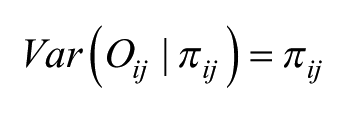
The approach introduced here develops from the literature on disease mapping where rates are often based on relatively small numbers of observations and so are inherently unstable – a small change in either or both of the numerator and denominator can substantially alter the rate (Clayton and Kaldor, 1987; Jones and Kirby, 1980). Any modelling of such rates must take into account the stochastic variation associated with small counts in some of the table’s cells by stabilising the incidence rates (Manda and Leyland, 2006).
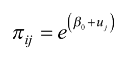
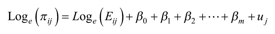
For each cell in the contingency table, we have an observed value. We can also calculate an expected value from a null hypothesis – the standard in much statistical hypothesis testing – that there are no differences across the cells in the rate being considered: thus, if we are looking at the propensity of individuals in the United Kingdom to vote either Conservative or Labour by sex and by age, if across the entire sample 45% vote Conservative, we would expect the same percentage in each age-sex group (e.g. both males aged under 25 and females aged over 65). We can then derive an observed relative rate for each cell, as the observed number divided by the expected: a ratio of 1.0 would indicate no deviation from the null hypothesis; rates above and below 1.0 would indicate cells with more or less persons than expected in them respectively if each subgroup voted the same way as all subgroups. Thus, by setting up the expected values in this way, we are identifying rates for voting – our outcome variable – in relation to age and sex as explanatory variables; if there were no differential effects of demography on voting, all the rates would be 1.0.
But how many more or less: are the differences from 1.0 likely to have occurred by chance or are they, in the standard statistical terminology, significantly different from 1.0 at some predetermined probability level? To address this question, we formulate a saturated (in the sense of a parameter for each and every cell of the table) Poisson regression model
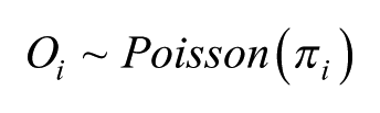
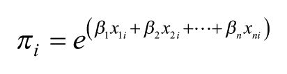
In this,
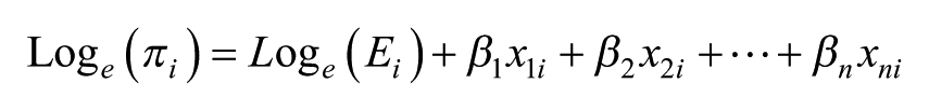
With the number of model parameters equal to the number of cells, this saturated model is not only unwieldy – especially in the case of a large table with many cells – but also little is gained as the exponentiated estimates are the same as the simple ratios of the observed to expected values in each cell; there is no pooling of information (Gelman and Hill, 2006) and each cell’s value is separately estimated – and there will be problems of fitting the model where the observed count is zero. Hence, instead we fit a random-effects two-level null or empty Poisson model

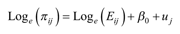
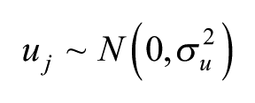
where individuals, i, are placed in the n cells, j, with an overall intercept,
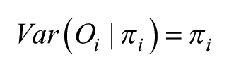
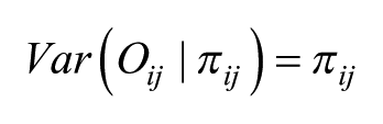
In the saturated fixed-effects model, normally specified by having a dummy variable for each cell in a regression framework, each cell’s value is separately calculated – only information from that cell is used to estimate the size of the effect – whereas in a random-effects model, as specified here, the estimates are precision-weighted, so that if they are based on small counts, the estimated rates are shrunk back towards the overall rate of 1.0 (that for the intercept) of the null hypothesis of no effect. The more unreliable the rate (i.e. the smaller the number of observations on which it is based), the closer it will be to 1.0 (Jones and Bullen, 1994). This is equivalent to the Bayesian pooling of information (Beck and Katz, 2007; Jones and Spiegelhalter, 2011), and represents a data-driven adaptive procedure for handling the uncertainty associated with sparse data (Gelman, 2014). Furthermore, the estimated rates for each cell have associated Bayesian credible intervals (CIs), and here we have used the 95% intervals to summarise the degree of uncertainty around the estimates. We call an effect ‘significant’ if the 95% CIs do not include the value of 1, so that the weight of the evidence is for a distinctively high or low rate. 2 If the CIs on the exponentiated scale include the value 1, we do not have strong evidence that the rate for such a cell differs from that for the overall relationship; there is no credible evidence for a particular age-sex combination to have a preference for a particular political party. The exponentiated estimates provide a natural interpretation of effect size so that 2 represents a doubling of the rate of vote for that group. This is much easier to interpret than the contortions required by the multinomial logit model.
Another important advantage of this random-effects shrinkage approach is in relation to multiple comparisons, which is at the heart of the induction problem of standard exploratory procedures. If you do enough testing, the chances of finding significant results increase rapidly. However, as demonstrated by Gelman et al. (2012), it is much more efficient to shift estimates towards each other rather than try to inflate the usual confidence intervals through a Bonferroni correction to control the overall error rate. Thus, shrinkage automatically makes for more appropriately conservative comparisons while not reducing the power to detect true differences. The final advantage is dealing with zero counts. With raw rates, if the numerator of a cell is zero, then the associated rate can only be zero. Moreover, if you calculate a saturated fixed-effects model with such a count, the estimate will fail to converge and you will get impossible, uninterpretable values (accompanied and signalled by exceptionally large standard errors). 3 But this does not happen in the random-effects approach; what does happen depends on the expected value. A zero based on an expected value of 1 means a quite different thing from a zero based on an expected value of 100 – for the former, it is uncertain whether the rate is really zero; for the latter, we can be quite confident in this inference. The random-effects estimate shrinks more towards the overall rate for the former than for the latter.
The models are run using Markov Chain Monte Carlo (MCMC) estimation (Jones and Subramanian, 2014) within the standard multi-level modelling software (MLwiN), and we have checked that the models have been run for sufficient time (a discarded burn-in of 5000 simulations followed by a monitoring phase of 500,000) to ensure convergence and to obtain reliable 95% CIs. We have used default priors to impose as little information as we can on the estimates so that the results are data-driven.
The approach illustrated: voting at the 2015 British general election
To illustrate the argument, we use the example of voting at the 2015 UK general election, by age, sex and educational qualifications, using data from the post-election wave of the British Election Study (BES) Internet panel survey. 4 Most studies have found that age and sex are related to party choice. Educational qualifications are used here as a proxy for social class – in part because of incomplete data on other possible measures (such as occupation and individual or family income); those with higher level qualifications in general are in higher status occupations and have higher incomes. It is generally accepted that social class has become a less important influence on voting choice in recent decades (see Whiteley et al., 2013), but it remains relevant (as the results presented here show). In any case, the goal of the present analysis is not to contribute substantially to appreciation of British voting patterns but rather to illustrate the advantages of the method proposed for uncovering substantively interesting and well-supported patterns that might not otherwise be found. Respondents were placed into four groups: those with no qualifications, those whose qualifications were only those associated with the official school-leaving age (in England formerly termed ‘O levels’ and now General Certificate of Secondary Education (GCSE)), those with post-school-leaving-age qualifications below the status of university degrees and diplomas, and those with degrees or diplomas.
For the analysis, we have excluded all respondents living in Scotland and Wales, where voters had a different set of outcome choices – the respective nationalist parties (the Scottish National Party (SNP) and Plaid Cymru) contested all seats there in 2015. (Northern Ireland is not included in the BES.) For England alone, therefore, we study those who voted for one of the five parties which contested virtually all of the seats, 5 plus those who reported that they did not vote. 6 The small number of BES respondents who voted for another party are excluded. This gives a sample size of 20,966 and a multivariate contingency table comprising six vote choices, two sexes, six age groups and four qualification categories – a total of 288 cells, giving an average of 73 respondents per cell. Nevertheless, many of the cells contained small numbers of respondents, as shown in Figure 1; the distribution is highly skewed (the median number of observations per cell was 44) – hence the value of the modelling approach adopted here that pools information to produce weighted estimates of rates in cells with small observed and/or expected values. To be clear, the expected value is derived for each age by sex by qualification group if the overall national rates of vote choice applied.
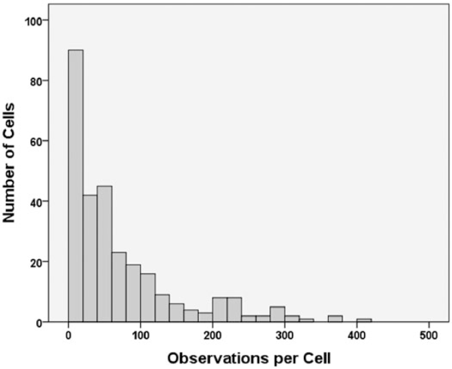
Histogram of the number of observations in each of the 288 cells of the sex by age by qualifications by vote contingency table.
The baseline
To provide a baseline for the application of our proposed method, we conducted multinomial logistic regression analyses with voting choice as the dependent variable, as would be the norm in studies of such contingency tables. Five models were run: the first three incorporated each of the ‘independent’ variables separately, the fourth included both age and sex and the fifth all three. The results – giving the regression coefficients and their standard errors, with significant differences from zero shown in bold – are presented in Table 1. The reference category for the dependent variable is voting Conservative, so each coefficient shows the probability of voting for another party rather than Conservative for the chosen group relative to its comparator. Thus, in Model 1, the first significant coefficient of −0.103 indicates on the logit scale that males were significantly less likely than females to vote Labour rather than Conservative.
Multinomial logistic regression models of voting in England in 2015, by sex, age and educational qualifications.
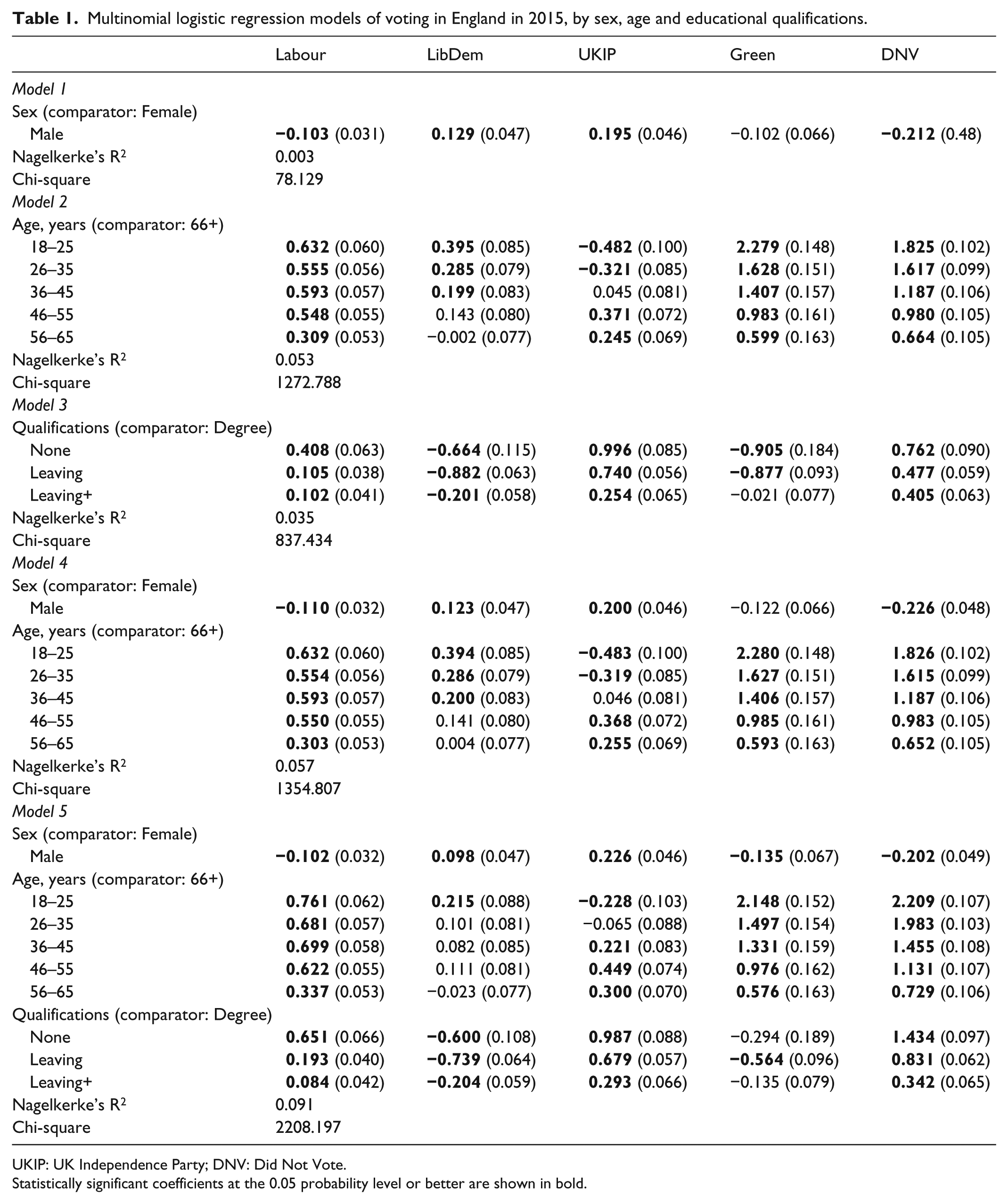
UKIP: UK Independence Party; DNV: Did Not Vote.
Statistically significant coefficients at the 0.05 probability level or better are shown in bold.
The overwhelming conclusion to be drawn from Table 1 is that all three independent variables are significantly related to voting choice – both separately and together. For example, males were less likely than females either to vote Labour rather than Conservative or to abstain rather than vote Conservative, and more likely to vote for either the Liberal Democrats or UK Independence Party (UKIP); there was no significant difference between males and females in their propensity to vote for the Green party. In general, younger people were more likely to vote Labour, Liberal Democrat or (especially) Green, or not to vote, rather than vote Conservative, compared to those aged 66 and over: those aged under 36 were significantly less likely to vote for UKIP rather than Conservative than those in the oldest age group, whereas those aged between 46 and 65 were more likely. There were also statistically significant and, given the varying size of the coefficients, substantial differences in voting by class. Those with no qualifications were more likely than those with degrees either to vote UKIP or to abstain rather than vote Conservative, for example.
For many studies, Table 1 would be the conclusion: significant patterns had been identified – very much in line with previous work and expectations. But two elements of that table raise questions. The first is the low level of ‘explanation’ provided by all the models: even Model 5, with all three independent variables included, accounts for less than 10% of the variation in voting choice – which leaves a great deal ‘unexplained’. That may well be because we have an under-specified model which excludes a large number of extra variables that other studies have shown to be related to voting choice (Whiteley et al., 2013). The second is the change in some of the coefficients – notably between Models 1–3 and 5. This is particularly the case with the age variables. Those for voting Labour rather than Conservative are substantially different between Models 2 and 5; those for voting Liberal Democrat rather than Conservative even more so – indeed, two that were highly significant in Model 2 are insignificant in Model 5. This suggests a degree of collinearity between age and qualifications, which may be confounding the ‘true’ relationships in the final model: members of some age groups may be more likely to vote Liberal Democrat in some classes than others.
These two issues together suggest that there may be interactions – that there are, for example, not only differences in voting by age and by sex separately but also by age and sex together. But an attempt to fit a Model 6 – introducing all of the possible two- and three-way interactions among the variables – failed because of singularities in the Hessian matrix resulting from the large number of cells with zero or near-zero values. It was not possible, therefore, to compare the outcome of our multi-level modelling (discussed later) with that of a multinomial regression incorporating the full set of possible influences on voting patterns – such as differences between age-sex groups within those with the same qualifications. 7 Furthermore, even if a Model 6 could be fitted, all of the one-way ratios together with the two-way and three-way interaction ratios have to be taken into account when determining the size of any significant differentials; interpretation is far from straightforward. Hence, the value of the approach adopted here, which generates a modelled rate, with CIs, for each cell – that is, for each of the six voting options, including Conservative, which is a comparator only in the multinomial regression model and for which there is no direct indicator of where its support is strongest and weakest. The method introduced here avoids those difficulties by providing a single coefficient for each cell of the n-way table being analysed, with an indication of whether it is significantly different from the null effect of 1.0 on the exponentiated scale; the output from the multi-level modelling is more readily interpretable.
Unpacking the table
Rather than explore the interactions through the multinomial logistic regression framework, therefore, we have analysed the 6 × 2 × 6 × 4 contingency table using the method introduced above. The output from this is 288 modelled rates, each with its Bayesian CIs, and these rates are shown in Tables 2 to 7 – one each for the voting choices. Table 8 and Figure 2 provide summaries of the number of significant rates – that is, those that are reliably different from 1.0, according to their CIs, for each category in each of the independent variables and for each of the voting choices.
The modelled values (with their CIs) for the rates of voting Conservative by sex, age and educational qualifications.
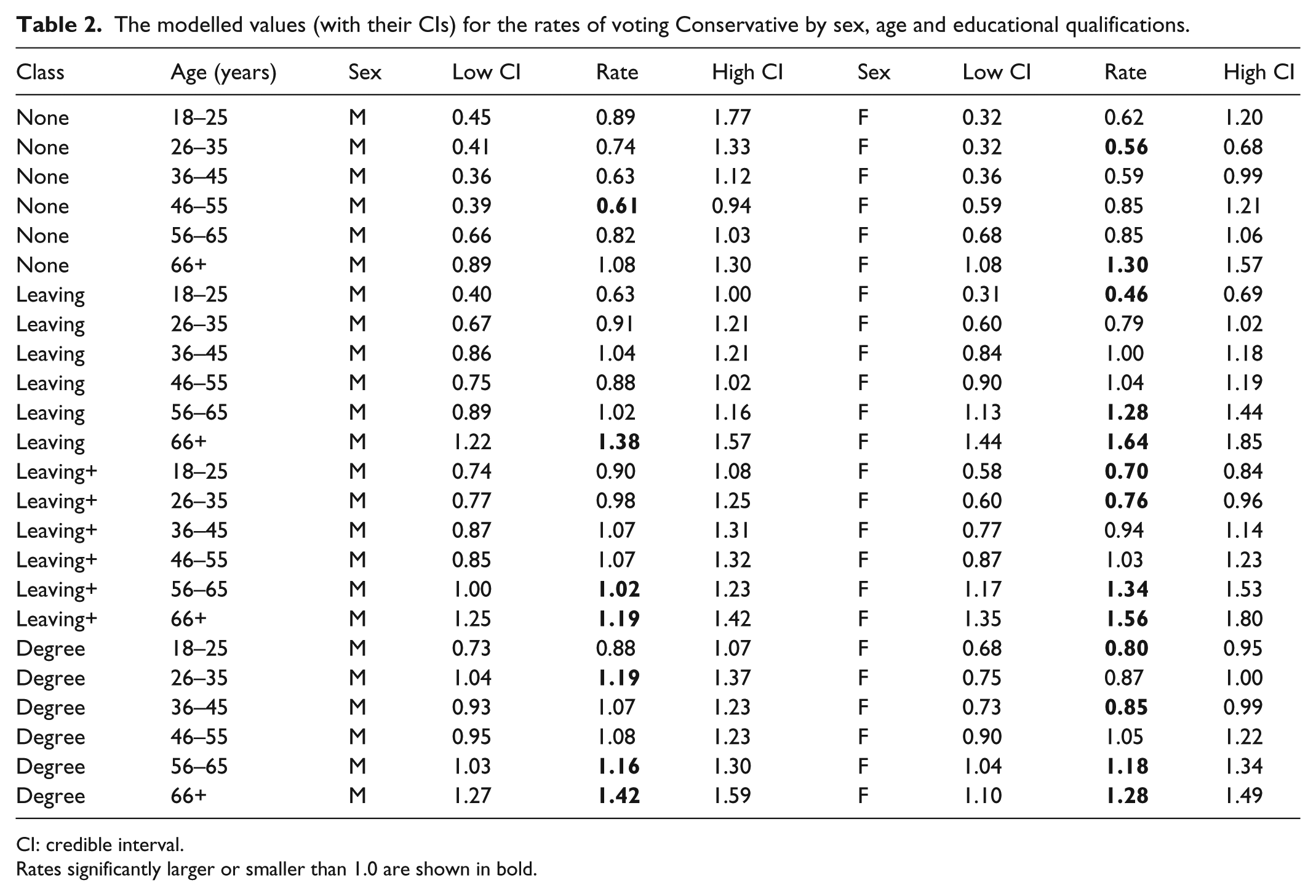
CI: credible interval.
Rates significantly larger or smaller than 1.0 are shown in bold.
The modelled values (with their CIs) for the rates of voting Labour by sex, age and educational qualifications.
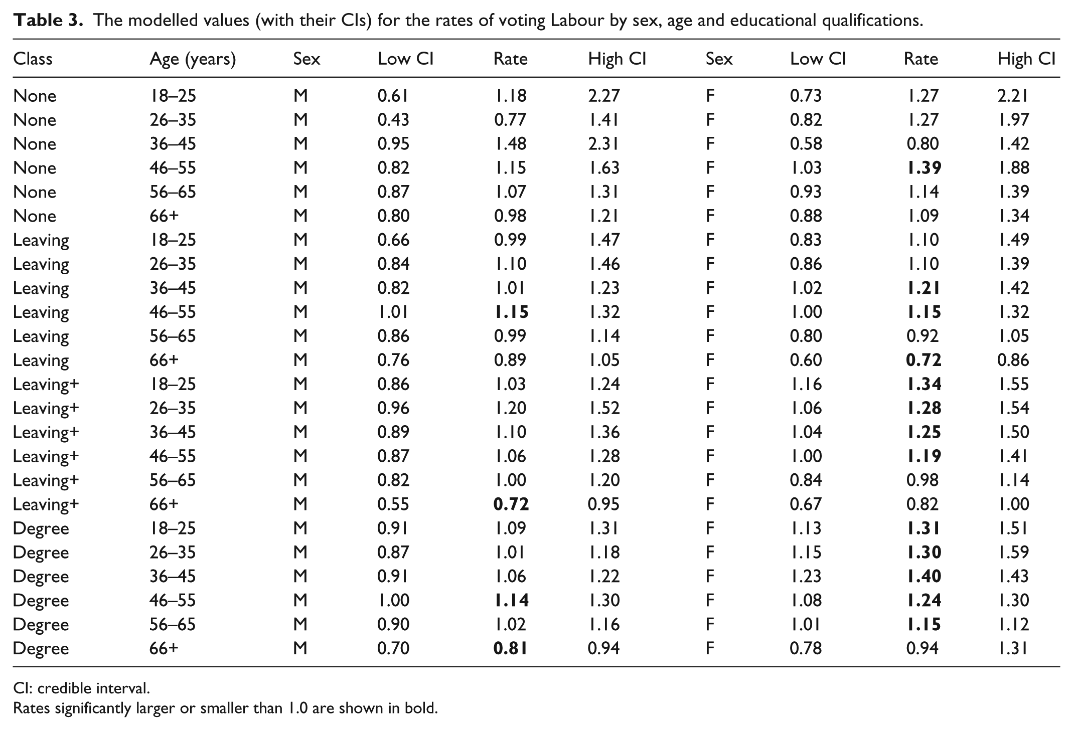
CI: credible interval.
Rates significantly larger or smaller than 1.0 are shown in bold.
The modelled values (with their CIs) for the rates of voting Liberal Democrat by sex, age and educational qualifications.
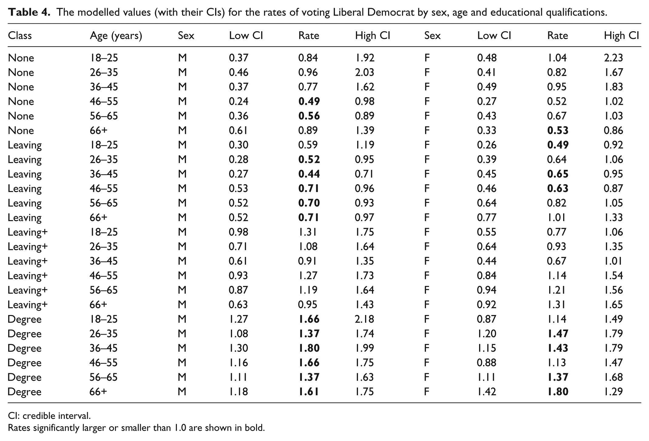
CI: credible interval.
Rates significantly larger or smaller than 1.0 are shown in bold.
The modelled values (with their CIs) for the rates of voting UKIP by sex, age and educational qualifications.
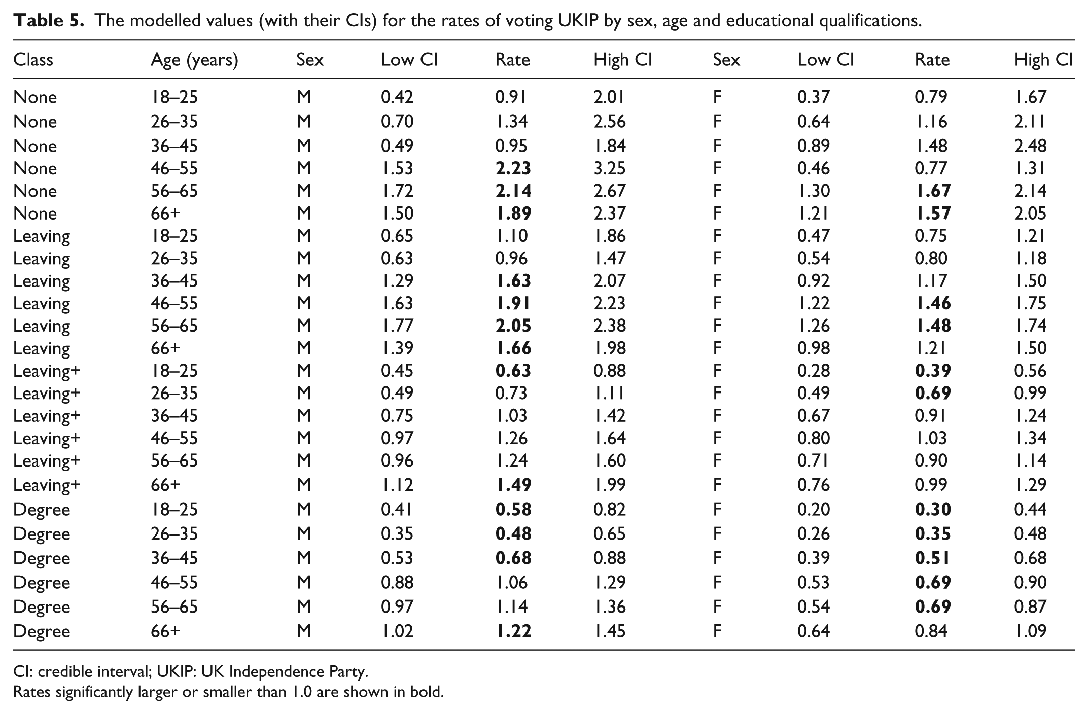
CI: credible interval; UKIP: UK Independence Party.
Rates significantly larger or smaller than 1.0 are shown in bold.
The modelled values (with their CIs) for the rates of voting Green by sex, age and educational qualifications.
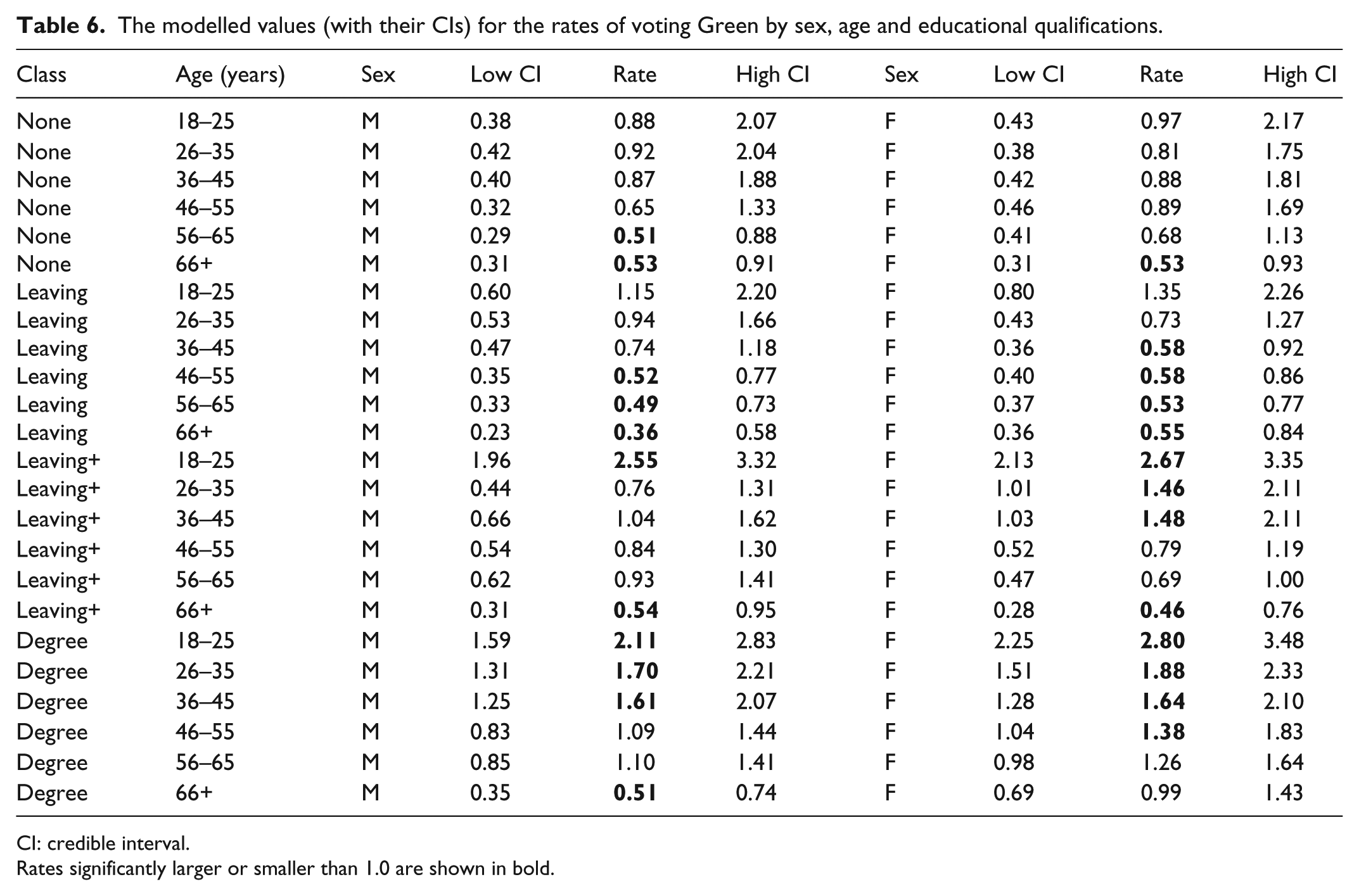
CI: credible interval.
Rates significantly larger or smaller than 1.0 are shown in bold.
The modelled values (with their CIs) for the rates of non-voting by sex, age and educational qualifications.
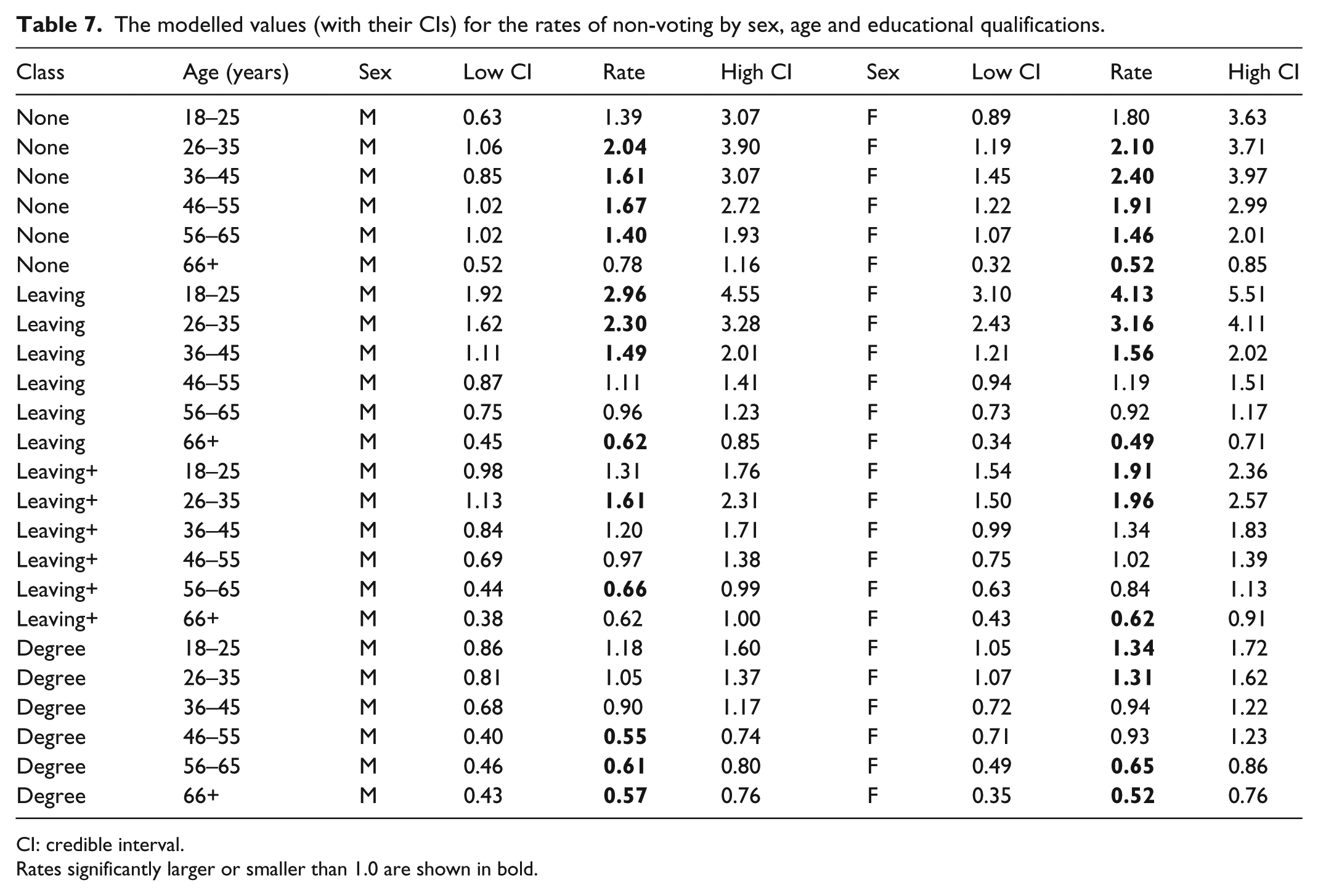
CI: credible interval.
Rates significantly larger or smaller than 1.0 are shown in bold.
A summary of the number of statistically significant modelled rates for each of the three sets of independent variables.
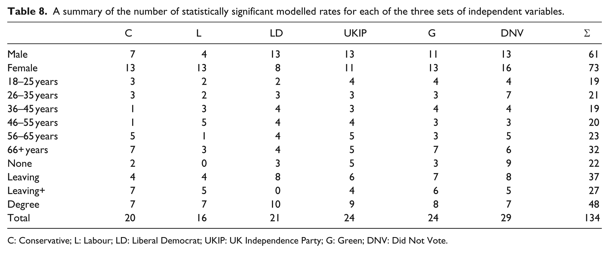
C: Conservative; L: Labour; LD: Liberal Democrat; UKIP: UK Independence Party; G: Green; DNV: Did Not Vote.
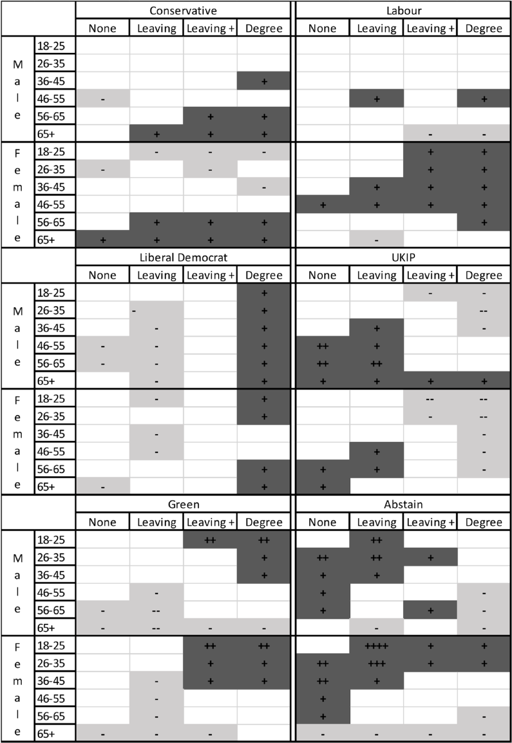
Diagrammatic depiction of the modelled voting outcomes. Cell values significantly larger than 1.0 are shown in dark shading; those significantly less than 1.0 are shown in light shading. (A + sign indicates a modelled rate of between 1.0 and 2.0; ++ indicates 2.0–3.0; +++ indicates 3.0–4.0; and ++++ 4.0<. A - sign indicates a modelled rate between 0.75–1.00; – indicates 0.50–0.75; – indicates 0.25–0.50; and —- indicates <0.25.
The expectation from the results of the multinomial regression analyses in Table 1, where virtually all of the coefficients are statistically significantly different from zero across all voting choices, is that Tables 2 to 7 should be replete with modelled rates that are also significantly different from 1.0 – that is, that there are significantly more or less individual respondents in each of the 288 cells of the multivariate contingency tables than expected. But only a minority (134) of the modelled rates is significantly different from zero. In part, this might not be unexpected because whereas the multinomial logistic regression results reflect the choice of a comparator among the categories in the independent variables, the approach outlined here does not – it reports modelled rates for every category. Thus, for example, Table 2 shows rates in the third qualifications category – those with qualifications beyond those obtained at the normal school-leaving age – among females that are significantly greater than 1.0 in the two oldest age groups and significantly less than 1.0 in the two youngest, but do not significantly differ from 1.0 in the two middle-age groups (36–45 and 46–55): the significant differences are not, as the multinomial model would have it, between one comparator group – the oldest – and all others, but have a U-shaped form.
Each of the six tables (Tables 2 to 7) has a very different pattern of significantly different rates. With voting UKIP (Table 5), for example, Table 1’s multinomial regressions suggested that males were more likely to support that party than females, that young voters were less likely to support it than their older contemporaries and that those with either no or few qualifications were more likely to support it than were those with degrees. Young, female degree-holders were thus least likely to be UKIP voters. The bottom block of modelled rates largely validates this expectation. For males, there are only three modelled rates significantly less than 1.0, whereas for females, there are five: for males, too, those aged over 45 were more likely to vote UKIP than expected – and significantly more so in the case of the oldest age group – whereas for females, all of the modelled rates were less than 1.0. Old, male degree-holders were more likely to vote UKIP than expected, whereas that was not the case with females.
Other cells in that table identify substantial, and in many cases statistically significantly different from 1.0, rates indicating differences that are not apparent from the multinomial regression. In both of the first two qualifications classes (those with either no or few qualifications), for example, older males were very much more likely to vote UKIP than females at all ages above 45. Among the highest qualified, on the other hand, males deviated less from the average rate than females; for males aged 18–25, the modelled rate was 0.58, whereas for females, it was 0.30. 8
The other tables also reveal patterns that the multinomial regression suppresses. In voting Labour, for example, there are only four modelled rates significantly different from 1.0 for males, but 13 for females. Whereas female voters in the higher two classes were much more likely to vote Labour than expected – except for those in the oldest age groups – compared to those 10 significant rates greater than 1.0, there was only one for males. Again, the fact that there were substantial differences between males and females, according to their age, in their propensity to vote Labour is not revealed by the multinomial regression. Strong support for both the Liberal Democrats and Greens is generally associated with the young and the better qualified – patterns shown in Table 1 and largely confirmed in Tables 4 and 6. Nevertheless, important differences emerge: female voters aged 26–45 in the third qualifications class were much more likely than comparable males to vote Green, for example, and there were significantly few degree-holding males in the oldest age group, but not females, supporting that party.
Many of the clearest differences are in the pattern of abstentions (Table 7). In general, young people, females and those with no or few qualifications were most likely to abstain (Table 1), but again the disaggregated approach promoted here adds detail to that general pattern. Among degree-holders, for example, significantly more young females than expected abstained, but that was not also the case among males in the comparable age groups.
The results of the multinomial logistic regressions provide no direct evidence regarding the pattern of voting Conservative – the chosen comparator among the dependent variables; this can only be inferred from the reported coefficients, or calculated from the associated odds ratios. With the method outlined here, however, the pattern of Conservative voting is part of the output (Table 2). As is the case with voting Labour (Table 3: see above), there are more statistically significant modelled rates for females (13) than for males (7). Furthermore, there appears to be greater polarisation in voting Conservative by age among females than males. In the first three qualification categories, for example, the difference between the modelled rate for females among the youngest and oldest age groups is greater than the comparable figure for males: among those with school-leaving qualifications, the modelled rate for those aged 18–25 is 0.46 for females and 0.63 for males (the former is also statistically significant), whereas the rates for those aged over 65 are 1.64 for females and 1.38 for males – a gap of 2.18 for females but only 0.75 for males.
Table 8 provides an overall summary of the number of statistically significant modelled rates in the preceding six tables. For each party and for non-voting, the total number of rates that could be significantly different from 1.0 is 48, but for only one of the six choices – not voting – is that the case in more than half. Voting Labour has only 16 significant rates – just one-third of the potential total; in general, the number of people voting Labour by age, sex and qualifications combined rarely differed from what would have been the case if voting was uniformly distributed across both sexes and all age groups and classes. Turning to the independent variables, there were more modelled rates statistically significantly different from 1.0 for females than males, more for the older and the younger than the middle-age groups, and many more for the highly qualified than for those with no qualifications.
Figure 2 provides an alternative summary procedure, from which the major patterns revealed by the significant modelled rates are readily appreciated. The clear age difference among females in their tendency to support either the Conservatives or Labour stands out, for example; younger females, especially those in the higher qualifications categories, are much more likely to vote Labour than Conservative (a difference that does not also apply to males), whereas older females, across all educational classes, are much more likely – like males – to vote Conservative. Among males, those with degrees were more likely than expected to vote Liberal Democrat, whatever their age, whereas those in the oldest age groups were more likely than expected to vote UKIP, whatever their qualifications. These differences between the sexes are not reproduced in either the pattern of voting Green or of abstaining, however, again stressing the importance of exploring the interactions: male–female voting patterns differed by age and educational class in some parts of the contingency tables but not others.
Exploring for significant interactions in a large contingency table produces a large volume of output, therefore – as Tables 2 to 7 illustrate. But the core of the exploration can readily be revealed by summary devices such as Table 8 and Figure 2. They point clearly to where the substantial interactions are, providing the foundation for further analysis and hypothesis-formulation. The precision-weighted effect sizes once the credible rates have been winnowed from the unreliable can be examined in detail to see both the overall patterns and interesting departures.
A hybrid model including fixed effects
The model we have so far fitted allows for the maximum differences in the random part. We now consider a hybrid model in which we additionally include estimated fixed effects for Vote (i.e. the six categories used previously – either support for one of the five parties or abstention) in interaction with Class, Age and Sex. This hybrid is a two-level random-effects Poisson model in which there are a set of fixed effects (

The Level 2 variance (
We formulated this model in the light of the findings summarised in Table 8 and Figure 2 and by examining residuals from a sequence of models with more complex fixed parts. That is, we included interactions on the basis of the detailed exploratory analysis we had undertaken, and we did this sequentially adding terms and looking for improvements in the model. This is judged in three ways. First, the smaller the residual variance (
A summary of a set of models of increasing complexity in the fixed part.
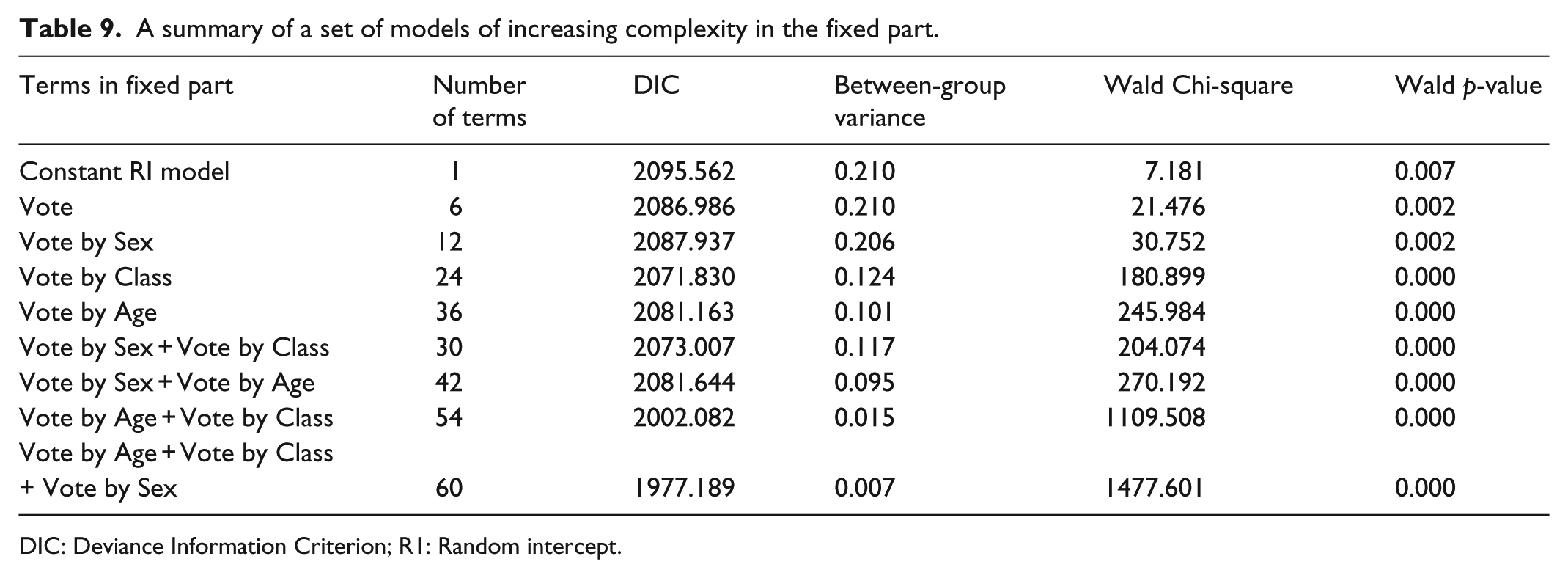
DIC: Deviance Information Criterion; R1: Random intercept.
The final model has 60 terms in the fixed part (representing Vote by Class + Vote by Age + Vote by Sex) that captures much of the variation and is a clear improvement on simpler models. The modelled fixed-part results are shown graphically (without CIs for clarity) in Figures 3 to 5; all three graphs have the same vertical scale so that the size of effects can be readily appreciated.
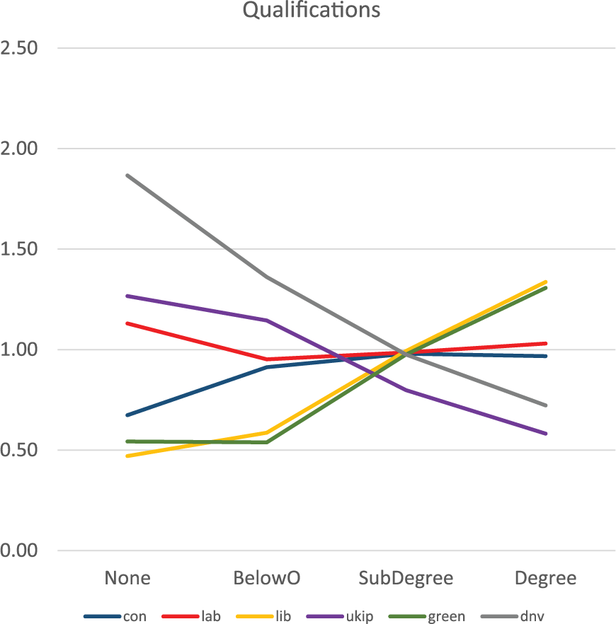
The modelled rates of voting for each of the five parties, or of not voting, by qualification levels, holding age and sex constant.
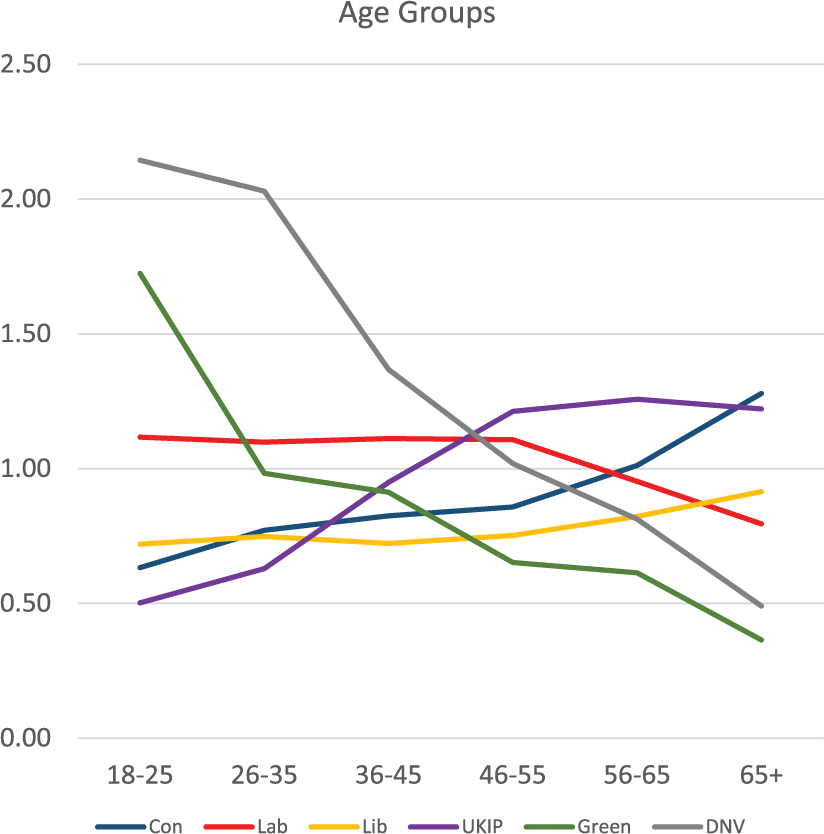
The modelled rates of voting for each of the five parties, or of not voting, by age, holding qualification levels and sex constant.
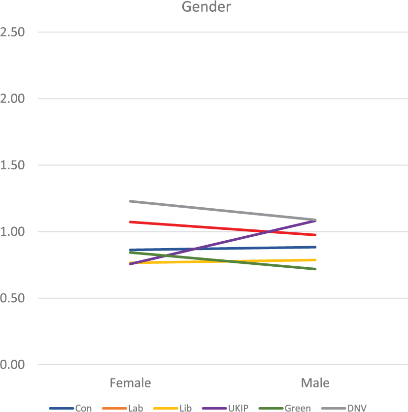
The modelled rates of voting for each of the five parties, or of not voting, by sex, holding qualification levels and age constant.
Figure 3 shows the estimated vote rate for each party in terms of the modelled rate for the educational classes when age and sex are kept constant at their average values. Three clear separate patterns stand out, each involving two of the six outcomes. Regarding both voting for either the Liberal Democrats or the Greens, there is a strong upward trend: holding age and sex constant, the likelihood of voters choosing one of those two parties increases according to their qualifications. Running in the opposite direction, the likelihood of somebody either voting UKIP or abstaining falls as qualification levels increase. Finally, for most qualification levels, voting either Conservative or Labour is invariant, with ratios close to 1.0; only among those with no qualifications is there any marked difference – they are more likely to vote Labour than Conservative.
Figure 4 shows the differences in average rates by age group, holding sex and qualification levels constant. Here, the dominant pattern is the decline – from rates of c.2.0 among those aged 18–25 to 0.56 for those aged over 65 – in the likelihood of not voting and also of voting for the Green party: the young were much more likely than expected to vote Green and also to abstain, with the inverse for the oldest age group. The likelihood of voting for both the Conservatives and UKIP increased with age; voting Labour declined among older people – once age and qualifications had been taken into account. Finally, Figure 5 shows that – compared to variations by age and qualifications – there were smaller differences between males and females in their propensity to vote for one of the parties, or to abstain. Males were less likely than females either to support two of the parties (Labour and Green) or to abstain; they were slightly more likely to vote either Conservative or Liberal Democrat and – by far the clearest difference shown – much more likely to vote UKIP.
By fitting these hybrid models, therefore, in which two of the three explanatory variables are held constant to display the average differences in the third, we have clarified the main patterns in voting by age, sex and class identified by the modelled rates. Inspection of the plotted residuals from this final model – not shown here – found that unaccounted differences were small and identified no other systematic regularities that might be indicative of other relationships that could be captured by further interactions in the fixed part. Indeed, the residual variance of the most complex supported model is only some 3% of the original variance.
Conclusion
This article has introduced an innovative modelling procedure for investigating differences in rates across all of the cells in a multivariate contingency table. Whereas standard procedures for analysing such tables – binomial and multinomial logistic regression – model the ratios of ratios, producing coefficients that are not directly interpretable, although their statistical significance can be assessed, the approach presented here provides greater clarity in its output. It models the rates in each cell separately but as part of an overall distribution, giving a clear statement of whether the rate there differs significantly from what would be the case under a null model, if each cell had the same proportion of its individual members in a particular category of the response outcome as the entire sample. Crucially, if the evidence for distinctive rates is unreliable, the rates are automatically shrunk back to a null value of no effect – we are protected from over-interpretation. But at the same time, reliable rates for even fine-grained tables can remain distinctive and point us to quite nuanced and detailed findings which we would not otherwise uncover.
The value of this approach has been illustrated using a relatively large (in terms of cells) multivariate table – though much smaller than are implicitly used in comparable tables in similar studies (as in Clarke et al., 2004, 2009; Whiteley et al., 2013) – regarding voting choices at the 2015 British general election. Although not designed to make a substantive contribution to British electoral studies, the results clearly illustrate the greater detail that the proposed approach provides relative to traditional procedures. It also draws attention to Elwert and Winship’s (2010) comment regarding the size of many social science surveys: that analysed here contained over 20,000 respondents, but many of the 288 cells in the four-way multivariate contingency table analysed had only a small number of observations. A method such as that used here which can compensate to some extent for that sparsity offers a substantial improvement over other procedures.
As emphasised at the outset of this article, much analysis in contemporary behavioural social science is, at best, quasi-exploratory; it tests general hypotheses regarding relationships rather than strong hypotheses regarding the direction and intensity of any such relationships, but – as Gelman and others have argued – rarely explores all of the potential relationships in such data sets because it ignores any interaction effects among the variables being considered. Furthermore, the methods generally deployed in such exploratory work – such as multinomial logistic regression – are limited in their applicability, as illustrated here, because the sparsity of values in many cells of the multi-way contingency tables typically analysed means that the full models incorporating all possible interaction effects cannot be fitted; and where there are no specific hypotheses indicating which interaction effects may be significant, the modelling cannot be limited to them alone. Hence the potential exploratory value of the multi-level-modelling-based approach introduced here. It is firmly based in Bayesian statistics, using a random-effects shrinkage approach, and generates modelled values for every cell of the multi-way table, each with its own CIs. Those modelled rates are readily interpretable and, as demonstrated in the case study deployed here, can be used to uncover differences within as well as between groups (the latter being all that a standard logistic multinomial regression without interactions can uncover); they explore the complexity of variation across the internal cells of a multi-way table rather than concentrating attention, as is so often the case, on its marginal totals alone.
Gelman argued that the exploratory search for interaction effects – characteristic of so much behavioural social science – should take advantage of the power of multi-level modelling. This article has applied and illustrated that contention. Its findings suggest that the approach – applicable within publicly available software – has wide application in the exploratory analysis of large multi-way tables across those disciplines. 10 Other means of identifying patterns within large multi-way contingency tables may well be suggested. This article has clearly set out one such novel procedure and identified its advantages over that widely used to analyse data sets such as that deployed here to illustrate the method and interpret its outputs. Its use allows patterns within data sets to be uncovered more effectively and thus offers a potential way forward in the appreciation of heterogeneity identified by a number of commentators as a substantial problem for quantitative social science.
Footnotes
Acknowledgements
We are grateful to the editor and three anonymous reviewers for their comments and advice on various versions of this article, especially to one reviewer whose challenging but constructive comments ensured clarity in our presentation of the hybrid model.
Declaration of conflicting interests
The author(s) declared no potential conflicts of interest with respect to the research, authorship and/or publication of this article.
Funding
The author(s) received no financial support for the research, authorship and/or publication of this article.