Sage Journals: Discover world-class research

Abstract

A “rhythmic agent” is simulated based on the foundation of a previously published behavioral sensorimotor synchronization (SMS) model. The model is adjustable to control the auditory and tactile modalities of the tap's feedback. In addition to the conventional mechanisms of phase and period error correction, as well as their activation conditions, the period is estimated by modeling a central timekeeper impacted by a novel short-term memory. Inspired by The ADaptation and Anticipation Model (ADAM), a mechanism for linearly extrapolating anticipation is also tested. To better match the perceptual and motor cognitive functions, the model's parameters have been tuned to observations from experimental neurosensory literature with an emphasis on transduction delays. The agent is programmed to synchronize with various external rhythmic input signals while accounting for both adaptive and predictive mechanisms. The definition of the agent is based on a minimal set of rules yet has successfully replicated results of real-world observations: against a metronome; it produces the well-known negative mean asynchrony. In a rhythmic joint action, the simulation of joint delayed coordination shows a behavior previously observed in human subjects: in a rhythmic collaboration, a moderate amount of delay is necessary to keep the tempo steady, and below that threshold, the rhythm tends to speed up. It is also shown that giving more weight to the tactile afferent feedback than the auditory intensifies this effect. Moreover, it is observed that including anticipation in addition to the reactive mechanism will decrease the effect. The proposed model as a rhythmic engine, combined with other standard modules such as a beat detection algorithm, can be used to implement musical co-performers that could improvise with a human rhythmically or perform a given score in a way that feels human-like.

Introduction

Behavioral studies in sensorimotor synchronization (SMS) have a long history (Blumenthal, 1975; Michon, 1967; Repp, 2005; Repp & Su, 2013) and, in general, are more mature than neurocognitive approaches to studying rhythm. To let the behavioral approaches benefit from existing knowledge in neuroscience and facilitate interdisciplinary discussions, it is valuable to connect the two bodies of knowledge (Buhusi & Meck, 2005). To explain the mechanisms underlying rhythmic behavior, recent neurocognitive studies have started to frame results from behavioral experiments (Keller et al., 2014; Nozaradan et al., 2018; Schultz et al., 2021; Schwartze et al., 2011). We will attempt to make such a link by looking at classic models of SMS while considering the peripheral properties of the body, such as transduction delays across auditory and tactile modalities. This work is a mathematical attempt to simulate the mechanisms behind synchronizing motor actions with sensory events in time. First, we provide a literature review of different approaches relevant to computational SMS. Then, a minimal set of rules are used to implement the structure of the agent and its algorithmic function, informed by the two bodies of knowledge mentioned earlier, neurosensory studies and behavioral SMS. Finally, the rhythmic agent is tested against different inputs, such as responding to a step change in tempo or performing with another agent. Where available, the results are compared with known experiments involving humans. The aim is to replicate the results of some known SMS experiments observed in previous research, namely its behavior in response to a simple metronome, a sudden tempo change, and rhythmic joint collaboration.

Traditionally, two main theoretical approaches are distinguished in the SMS literature (Repp, 2005): the information-processing approach usually models responses with event-based discrete time series and focuses on cycle-to-cycle error corrections. On the other hand, approaches inspired by dynamic systems theory (Large, 2008) represent movement as a trajectory in phase space and deal with continuous, nonlinear, and within-cycle coupling (Repp, 2005).

In the former approach, synchronization to external rhythmic stimuli is typically controlled by two error correction processes which are “asynchrony-based” and “interval-based” (Schulze et al., 2005). The first process, the phase correction mechanism, corrects phase error (asynchrony), is considered mostly automatic and unconscious, and does not affect the tempo (Repp, 2001a; Repp & Penel, 2002). The latter process, period correction, is usually intentional and deals with the discrepancy, that is, errors in intervals and changes in tempo (Repp & Su, 2013).

Recently, hybrid models have evolved to incorporate elements from each approach, such as following the classic adaptive formulation of phase-correction, while modeling period correction dynamically (Loehr et al., 2011). Models based on continuous-time dynamical systems can also incorporate event-based error correction rules (Large et al., 2023). Since the classical pacemaker accumulator models do not reveal the neural mechanisms of counting pulses (Zemlianova et al., 2022), continuous-time neuromechanistic models combine error-correction with neuronal entrainment concepts by achieving internally generated timings from parameters of a dynamical neuronal system. In a biophysically-based neuronal framework, Bose et al. (2019) showed that a neuronal-level oscillator could learn both the period and phase of an external isochronous rhythm by utilizing discrete clocks formed by gamma rhythms and synchronizing spike times to achieve rhythmic timekeeping across a range of musically-relevant frequencies. Byrne et al. (2020) proposed a neural system that could adapt its oscillatory behavior through iterative error-correction of internal parameters, described by a two-dimensional event-based map.

In this work, in line with the former, information-processing approach, we will base the formulation of a rhythmic agent on a cycle-to-cycle design. We assume a central timekeeper to keep track of time events and intervals and apply linear error correction of phase and period to synchronize the motor commands to an external stimulus sequence (Vorberg & Schulze, 2002; Vorberg & Wing, 1996). The terminology and the choice of variables primarily follow the model Mates developed in his twin papers, explaining the synchronization mechanism between motor actions and sensory events (Mates, 1994a, 1994b). In addition to the conventional adaptive/reactive mechanisms of phase and period error correction, we have incorporated a separate mechanism of period estimation based on the impact of a novel, optional, short-term memory on the central timekeeper. Following the framework laid out by (Van Der Steen & Keller, 2013) in their ADaptation and Anticipation Model (ADAM), we have also tested the anticipatory mechanisms involved in SMS through linear extrapolation. We have chosen the model's parameters based on experimental literature by recent references to anatomical and neurosensory studies to quantify the model constants. In contrast with the recent neuromechanistic models, instead of investigating the dynamics of beat generation at a neuronal level, we will focus on the biophysical properties of transduction delay.

The Model

The agent's architecture in Figure 1 is inspired by the anatomical structure of a human performer and the connections between the parts involved in the synchronization task. The input sequence, $S (k)$ , represents the timestamp of the received kth onset of a stimulus during an SMS task. For the output sequence, $R (k)$ denotes the timestamp of the performed response to $S (k)$ , representing a one-to-one (1:1) SMS task. The model parameters in this figure are related to the peripheral nervous system (PNS), are listed in Table 1, and are quantified given literary references to neurophysiological studies; however, the agent's algorithmic design is based on the literature on behavioral SMS.

Figure 1.

The structural architecture of the SMS agent used in the simulation.

Table 1.

Variables involved in the structure of the SMS agent.

Notation	Name	Description
$S (k)$	Stimulus	Timestamp of the kth stimulus onset
$R (k)$	Response	Timestamp of the kth response onset
$τ_{a i r b o r n e}$	Airborne sound delay	Delay for airborne sound from hands to ears
$u_{I}$	Auditory transduction delay	Auditory transduction delay for both stimulus and response
$f_{I, t a c t i l e}$	Tactile transduction delay	Transduction delay in tactile feedback of an already performed response
$F_{I} (k) = R (k) + f_{I}$ $f_{I} = λ (τ_{a i r b o r n e} + u_{I}) + (1 - λ) f_{I, t a c t i l e}$	Mean feedback transduction delay	Effective compromise between auditory and tactile feedback of the performed response $R (k)$ , based on the variable $λ$ implemented
$m_{I}$	Motor delay	Delay in execution of a motor act
$S_{I} (k) = S (k) + u_{I}$	Click	Central auditory representation of stimulus $S_{j}$
$F_{I} (k) = R (k) + f_{I}$	Tap	The central feedback of the performed response which includes tactile and auditory representations of response are unified
$R_{I} (k) = R (k) - m_{I}$	Motor command	Initiation of the jth motor command
$s (k) = S (k) - S (k - 1)$ $= S_{I} (k) - S_{I} (k - 1)$	ISI = ICI	Inter-stimulus interval = inter-click interval
$r (k) = R (k) - R (k - 1)$ $= R_{I} (k) - R_{I} (k - 1)$ $= F_{I} (k) - F_{I} (k - 1)$	IRI = ITI	Inter-response interval = inter-tap interval

Description of the Variables

Mates’ notation is widely used in SMS research and is followed in this paper too. He described the temporal data from an SMS task either by event variables (“reading of a clock”), denoted by capital letters, or interval variables (temporal differences between two events) symbolized by lower-case letters. For example, $S (k)$ is the timestamp of the kth stimulus onset in a one-to-one synchronization task and $s (k)$ represents the length of the inter-stimulus interval (ISI), the time between two consecutive events $S (k - 1)$ and $S (k)$ . Similarly, the timestamp of the response to this stimulus is denoted by $R (k)$ . The temporal difference between $R (k)$ and $R (k - 1)$ is known as the inter-response interval (IRI),¹ symbolized by $r (k) :$

s (k) = S (k) - S (k - 1), r (k) = R (k) - R (k - 1)

(1)

The Internal Representation of the External Events

Concerning the notion of the dedicated timekeeper in the information-processing framework, external and objective temporal events are assumed to have internal representations in the central nervous system (CNS).² The distinction between the internal and external events in neurocognitive studies has roots in the “perception latency hypothesis”: there is a delay between stimulus input and the temporal availability of its representation in the CNS (Pöppel et al., 1990). Literature indicates two main theories to explain such delays in perception: the “nerve conduction hypothesis” (Paillard–Fraisse hypothesis) and the “sensory accumulator model” (SAM). The nerve conduction hypothesis accounts for neural transmission delay of the sensory information as the primary source of the perceived latency (Aschersleben, 2002). Alternatively, the more comprehensive SAM attempts to explain such latencies based on the central processing time of perceptual information (Fraisse, 1980; Repp & Su, 2013), instead of the peripheral conduction time. The simulation in this study is more in line with the nerve conduction hypothesis, where such lags are the results of constant transduction delays. Therefore, the neural transmission delay of the sensory input or other time-consuming processes of information is reduced to a constant temporal delay that bridges between the external variables and their central representation. Small boxes in Figure 1 represent these delays. We will attempt to quantify them with a value, or a range of values, informed by experimental literature. Note that in an SMS task that does not incorporate the visual channel, the transduction delay can appear only in auditory and tactile forms.

In Mates’ terminology, both events, $S (k)$ and $R (k)$ , and intervals, $s (k)$ and $r (k)$ , represent the events outside the human body; hence, they are externally measurable in a lab. The internal representation of these events and intervals are to be perceived by the performing subject (Table 1). The internal representation of the stimulus, $S (k)$ , is denoted by $S_{I} (k)$ , and is called click. Studies show that the assimilation in paired musicians is dominated by the auditory channel, with the effects of visual information being negligible (Nowicki et al., 2013). Therefore, in the absence of the visual channel, $S_{I} (k)$ will be delayed only by an auditory transduction delay of $u_{I}$ :

S_{I} (k) = S (k) + u_{I}

(2)

In our model

u_{I}

is assumed to be a constant offset for a given agent and one can attempt to quantify it. The process of sound capture by the eardrum into action potentials in the auditory nerve takes 1–3 ms (Cullen et al., 1972; Margolis et al., 1992). In addition, at least five components of click-evoked electroencephalogram (EEG) signals with delays below 8 ms are typically distinguished after an auditory stimulus (Lieberman et al., 1973; Picton et al., 1974; Pratt & Sohmer, 1976). Hence,

u_{I}

could range from 1 to 8 ms.

The response $R (k)$ has two central counterparts: the preceding initiation of the motor command, $R_{I} (k)$ generated in the CNS which triggers the response, and the succeeding temporal central availability of feedback, which is the representation of the already generated response in the CNS. We denote this internal event variable with $F_{I} (k)$ .

(Roman et al., 2019) has accounted for the presence of auditory feedback from one's own produced onsets, using similar hypotheses as the current work, and by simulating an oscillator receiving its own delayed activity as input. However, $F_{I} (k)$ is a multisensory event resulting from combining the inputs from several sensory channels: auditory, visual, and tactile (Comstock & Balasubramaniam, 2018). Whereas we modeled $S_{I} (k)$ only including its auditory component, even in the absence of the visual channel, $F_{I} (k)$ still comprises both auditory and tactile elements. Situations where the feedback consists only of a tactile component have been tested by removing the auditory self-feedback in pairs of musicians, non-musicians, and mixed pairs performing together, showing that all pair types were better at maintaining the rate with the auditory feedback than with no feedback (Schultz & Palmer, 2019). The auditory feedback of the generated response is delayed by $u_{I}$ in equation (2) plus an airborne delay of $τ_{a i r b o r n e} = \frac{343 m / s}{0.34 m} \approx 1 ms$ , which is the time it takes for the sound to travel in the air from the hands to the ears, given the speed of sound in air and an average distance of 34 cm from hand to ear, that is, the auditory feedback takes place at $R (k) + τ_{a i r b o r n e} + u_{I}$ .

The tactile feedback element, on the other hand, is delayed by a tactile transduction delay of $f_{I, t a c t i l e}$ and hence occurs at $R (k) + f_{I, t a c t i l e}$ . An ignorable part of the tactile delay is caused by mechanoreceptors (sensory receptors that respond to mechanical pressure or distortion) in the “Pacinian corpuscle” (the main sensory receptors of human skin), reported as low as 0.2 ms (Kruger & Michel, 1962). To quantify the significant component of tactile transduction delay, considering the nerve conduction velocity (NCV), we look at the speed of electrical conduction of the motor and sensory nerves in the body. Norris et al., (1953) reported a conduction velocity of approximately 55 m/s for the “ulnar” nerve which runs through the arm and innervates³ the little finger and ring finger. Kruger reported conduction velocities for different sensory nerve signals in a range between 25 and 91 m/s, with a mean of 58 m/s (Perl & Kruger, 1996). Trojaborg reports bidirectional conduction velocities of the median nerve (innervating parts of the hand, including the index finger) and ulnar nerve to be approximately 55 m/s using different measuring methods (Trojaborg, 1964). When considering a mean, bidirectional NCV around 55 m/s or 58 m/s, the tactile feedback from the fingers would arrive in the CNS with a delay of approximately $f_{I, t a c t i l e} = 14$ ms for an average person with an arm length of 75 cm (Goel & Tashakkori, 2015; Kamal & Yadav, 2016).

The two afferent,⁴ auditory and tactile, representations of a response, respectively delayed by the values $τ_{a i r b o r n e} + u_{I}$ and $f_{I, t a c t i l e}$ , will be unified in the brain to produce the experience of the same event (Aschersleben et al., 2001). The effective delay could be modeled as a compromise between these two delays, using a weighted average with a hypothetical ratio of $0 \leq λ \leq 1$ . So, an effective feedback transduction delay ( $f_{I})$ is the time it takes for the performed response to be internally represented in the CNS, as a hypothetical internal event called tap and denoted by $F_{I} (k)$ :

F_{I} (k) = R (k) + f_{I}, f_{I} = λ (τ_{a i r b o r n e} + u_{I}) + (1 - λ) f_{I, t a c t i l e}

(3)

In addition to the sensory delays, Mates and others have included the delay involved in the execution of the motor command, denoted by

R_{I} (k)

(Mates, 1994a, 1994b; Wing & Kristofferson, 1973):

R_{I} (k) = R (k) - m_{I}

(4)

Similar to equation (1), which defines intervals for external variables, we can present interval variables (denoted by small letters) based on the time difference between two consecutive internal representations of those events. The assumption that transduction delays rely on constant physiological properties and do not vary over time implies that the internal representations of the stimuli are not temporally distorted and maintain the same time difference as the external ISI:

s_{I} (k) = S_{I} (k) - S_{I} (k - 1) = s (k)

(5)

Similarly, the internal representation of the response (as well as that of the motor command) will take on the same value as IRI. In other words, although we arrive at different external and internal representations for the event variables due to the offsetting delays, intervals mathematically maintain the same internal and external representations:

F_{I} (k) - F_{I} (k - 1) = r (k)

(6)

R_{I} (k) - R_{I} (k - 1) = r (k)

(7)

Initiation of the Next Motor Command

After presenting the agent's structure, we discuss its function by modeling the inner working of the CNS box in Figure 1. CNS is the main component in the modeling of the motor system's dynamic behavior in planning and control (Wolpert et al., 1995). An information-processing approach assumes that the output of this component, the trigger of the motor act, is merely determined by the received stimuli and performed responses, or in our model from their internal representations. In this section, we explain the algorithmic inner working of the model of the CNS.

The CNS module in Figure 1 calculates the next motor trigger as a function of previously observed stimulus and response streams of data. This function defines the SMS model in use and is usually expressed in terms of external events. Here, we present it based on historical values of two sequences of internal events, the feedback from an already performed sequence, $F_{I} (1)$ to $F_{I} (k)$ , and the internal representations of stimuli onsets, $S_{I} (1)$ to $S_{I} (k)$ . In agreement with Mates, we assume that the CNS determines the (internal) timestamp of the next motor trigger, $R_{I} (k + 1)$ , which is initiated $m_{I}$ ahead of $R (k + 1)$ , as the sum of the previous motor command, $R_{I} (k)$ , and a default interval, $\hat{t} (k + 1)$ , plus a correction term that we call $Δ$ :

R_{I} (k + 1) = R_{I} (k) + \hat{t} (k + 1) + Δ + τ_{j i t t e r}

(8)

Note that the performance of the agent is also “jittered” by adding a random temporal perturbation taken from a Gaussian distribution with a standard deviation of 5–20 ms and a mean of zero to the final timing of the response (Elliott et al., 2010). Since both the feedback and the motor initiation of the response are offset by the same constant delays (see equations (6) and (7)), equation (8) could also be written based on the response feedback,

F_{I}

, instead of the motor command,

R_{I}

(see Figure 2):

F_{I} (k + 1) = F_{I} (k) + \hat{t} (k + 1) + Δ + τ_{j i t t e r}

(9)

Figure 2.

Timeline of the events and intervals used to decide the motor trigger, $R_{I} (k + 1)$ , for the calculation of the next motor command, through the default interval $\hat{t} (k + 1)$ , which is set to the central interval, ${\tilde{t}}_{I} (k)$ , and is corrected by the term $Δ (S_{I} (k), F_{I} (k), {\tilde{t}}_{I} (k))$ , and jittered by Gaussian random variable $τ_{j i t t e r}$ . Note that the correction term, $Δ$ , captures the role of adaptation since it is calculated based on reactive error correction models (see equation (20)), and the central interval ${\tilde{t}}_{I} (k)$ is tunable between the input or output intervals (equations (10) and (11)), and includes the role of short-term memory (equation (13)).

Central Interval

In a one-to-one SMS task, $S_{I} (k)$ and $F_{I} (k)$ arrive at the CNS temporally close to each other, but not quite simultaneously. Even if the temporal mismatch between the internal representation of the input stimulus and the internal feedback of the generated tap is detectible, the CNS unifies the two corresponding events to perceive them as one internal event. Similar to Vos and Helsper (1992), who defined a linear weighting of the external stimulus and response, here we use a weighting parameter ( $0 < η < 1$ ) called the degree of attention to compromise between the internal representations of the stimulus and the response, click and tap. We call this internal variable a tick⁵ and denote it by $T_{I} (k)$ :

T_{I} (k) = η S_{I} (k) + (1 - η) F_{I} (k)

(10)

The tick is the unifier of the central availability of stimulus and response and, therefore, an internal event. As other events, it can have its own interval variable (similar to equations (5)–(7)), which we view as the interval of the central timekeeper, calling it the central interval and denoting it by

t_{I} (k)

t_{I} (k) = T_{I} (k) - T_{I} (k - 1) = η s (k) + (1 - η) r (k)

(11)

In formula (11), when

η = 1

, the central timekeeper focuses on the interval of the input stream received through the sensory channel, and the CNS only follows the input sequence. This setting reflects the notion of stimulus-driven or externally paced (exogenous) rhythmic behavior (Zamm et al., 2015 , 2016). At the other extreme, when

η = 0

, as if the agent is not paying attention to the incoming sequence, the tick takes the value of

F_{I} (k)

, representing self-driven rhythmic behavior (endogenous) hypothesized to originate from central pattern generators and reflected by a spontaneous motor tempo (SMT) (Roman et al., 2023). In this computational model, SMT acts as an attractor state, influencing the agent's internal tempo even without external cues. This aligns with the observation in human music performance, where musicians tend to drift back to their natural SMT when playing without a metronome. The parameter

η

can be defined with variations during a trial (dynamic) or be kept constant (static). A dynamic

η

, hence, captures the attention paid to the input sequence by the agent at a point in time. This parameter can account for the quantification of the strategy (Darabi et al., 2010b) as an example of higher cognitive mechanisms involved in SMS, such as the intentionality of a co-actor (Mills et al., 2019), musical expertise (Schultz & Palmer, 2019; Wolf et al., 2018), or individual skills (Mills et al., 2015) (Table 2).

Table 2.

Variables involved in the function of the SMS agent.

Notation	Short name	Unit	Description
$η$	Degree of attention	1	The degree to which the central timekeeper's hypothetical event onset (tick) relies on the externally received click as opposed to self-initiated tap.
$T_{I} (k) = η S_{I} (k) + (1 - η) F_{I} (k)$	Tick	ms	Central timekeeper's hypothetical onset, defined based on a balance of $η$ in the range between click and tap.
$t_{I} (k) = η s (k) + (1 - η) r (k)$	Central interval	ms	The interval of the central timekeeper (before the effect of short-term memory). Central interval turns out to be the balance between ISI and IRI by the same $η$ , that is, compromise between received stimulus intervals and performed response intervals ^a
$Ψ_{n} (a) = \frac{a - 1}{a^{n} - 1} [a^{n - 1}, a^{n - 2}, \dots, a, 1]$	Memory vector	1	A geometric progression with the scale factor of k and length of $n$ adding up to one
${\tilde{t}}_{I} (k) = [t_{I} (k - n + 1), \dots, t_{I} (k)] . Ψ_{n} (a)$	Central interval (with the role of memory)	ms	The inter-click intervals weighted with the memory vector $Ψ_{n, a}$
$e (k) = R (k) - S (k)$	External asynchrony	ms	Phase error based on the mismatch between external input and output events, stimulus and response
$e_{I} (k) = F_{I} (k) - S_{I} (k) = e (k) + f_{I} - u_{I}$	Internal asynchrony	ms	Phase error based on the mismatch between the central representation of stimulus and response
$d (k) = \frac{{\tilde{t}}_{I} (k)}{s (k)} - 1$	Discrepancy	1	Period error based on the mismatch between output and input intervals, IRI and ISI
$\hat{t} (k + 1)$	Default interval	ms	The default IOI planned for the execution of the next tap, before applying correction mechanisms
$Δ$	Correction term	ms	Correction term based on the observed errors from historic data
$α$ in $(Δ = - α e_{I} (k))$	Phase error correction gain	1	The correction proportion used to correct the latest perceived asynchrony
$β$ in $(Δ = - β d (k) s (k))$	Period error correction gain	1	The correction proportion used to correct the latest perceived discrepancy
$δ_{p h a s e}$ $(- δ_{p h a s e} < e_{I} (k) < δ_{p h a s e})$	Asynchrony tolerance threshold	ms	The time constant defining the range of t asynchrony (phase error) Toleration range
$- δ_{p e r i o d}$ $- δ_{p e r i o d} < d (k) = \frac{r (k)}{s (k)} - 1 < δ_{p e r i o d}$	Discrepancy tolerance ratio	1	The percentage defining the range of discrepancy (period error) toleration range
$τ_{j i t t e r}$	Jitter	ms	Random temporal perturbation (Gaussian)
$θ$	Initial tempo	bpm	The initial tempo at the start of a trial

With central timekeeper interval being $t_{I}$ we can define 60/ $t_{I}$ as central timekeeper's tempo in bpm.

Tranchant et al. (2022) makes a distinction in this regard between musicians and musically untrained individuals. They show that in non-musicians, relying more heavily on the innate spontaneous production rates (lower $η$ ) can cost a higher asynchrony in joint musical coordination. On the other hand, musically trained individuals demonstrate higher attention to their partner's rates and their higher temporal flexibility is associated with decreased endogenous constraints on production rate (higher $η$ ) and, therefore, greater interpersonal synchrony.

Short-Term Memory

In musical terminology, tempo is defined as the speed or pace of a given rhythmic piece. For an isochronous sequence of stimuli $S (k)$ , expressed in seconds, where all $s (k)$ intervals are constant, the objective tempo would be $60 / s (k)$ , in beats per minute (or bpm). When the sequence changes pace, the current pace is still calculable from the length of the intervals at a given time/index. According to the section “Central interval”, in an SMS task, where the agent deals with two potentially different values for ISI and IRI, the current pace of the rhythm can be defined based on a unified central interval, estimating the tempo at around $60 / t_{I} (k)$ bpm.

The central interval used here still does not account for the role of short-term memory, since it is only based on the last interval.

Several memory models incorporate a “decaying factor” to explain how information fades in short-term memory with time. Exponential decay is an arbitrary function used to represent such decline in the probability of information retrieval (Atkinson & Shiffrin, 1968) or in remembering a sequence of numbers in short-term memory (Shepard & Teghtsoonian, 1961). This function can also be observed in the context of auditory memory, such as in the loudness of a recently heard tone in short-term memory (Lu & Sperling, 2003) or the recurrence frequency of a song as involuntary musical imagery (Byron & Fowles, 2015). Although we did not discover a specific source detailing a time-based exponential decay for weightings of recent intervals in tempo inference, we were inspired by its appearance in other contexts and generalized our model by incorporating the role of short-term memory in accounting for the current tempo.

To implement, we took the n most recent IOIs as a vector and their weighted average as another vector with the same length n, called memory vector, $Ψ_{n}$ , which sums up to 1. For example, if we want to take a moving average of the last n intervals, the memory vector will be a uniform distribution, that is, $Ψ_{n} = [\frac{1}{n}, \dots, \frac{1}{n}]$ . An exponentially decaying function will then assign a geometric progression to this vector, with a scale factor of $a > 1$ so that it sums up to 1:

\begin{aligned} Ψ_{n} (a) & = \frac{a - 1}{a^{n} - 1} [a^{n - 1}, a^{n - 2}, \dots, a, 1], \\ a > 1 \in ℜ, n \geq 1 \in ℵ \end{aligned}

(12)

We can now model the perceived pace of a heard sequence of

S_{I}

and a performed sequence of

F_{I}

, with the corresponding unified events of

T_{I}

and unified intervals of

t_{I}

(see equations (10) and (11)), with

60 / {\tilde{t}}_{I}

instead of

60 / t_{I}

, where

{\tilde{t}}_{I}

is the inner product of a vector consisting of the last n unified intervals with the memory vector of the same length:

{\tilde{t}}_{I} (k) = [t_{I} (k - n + 1), \dots, t_{I} (k)] \cdot Ψ_{n} (a)

(13)

This period estimation based on a central timekeeper and short-term memory is not a substitute for correction mechanisms as suggested by Hary and Moore (1987). The estimated period (the central interval) will not replace the period correction but will account for the perception of the current rhythm, where a separate mechanism of period error correction will be applied to it.

Calculating the Planned Interval

The default interval of equations (8) and (9) can take the value of the last received ISI, that is, $\hat{t} (k + 1) = s (k)$ (Michon, 1967), the last tapped interval, ITI, that is, $\hat{t} (k + 1) = r (k)$ (Vos & Helsper, 1992), or the unified interval, that is, $\hat{t} (k + 1) = t_{I} (k)$ (Hary & Moore, 1987; Mates, 1994a, 1994b). Following the latter, we include the role of the short-term memory, to set the value for the next default interval:

\hat{t} (k + 1) = {\tilde{t}}_{I} (k)

(14)

Next, we set the initial values. At the start of a simulating trial, that is,

k = 0

{\tilde{t}}_{I} (0)

does not have a value, so we give it an initial value depending on the SMS task. In addition, when it comes to the first generated response, the starting value of the first motor command without the historic values can be set to

R_{I} (0) = τ_{j i t t e r}

The correction term, $Δ$ , is at the heart of the SMS model and captures how the agent adjusts the timing of the performed tap to minimize certain cost functions that are key to the performance of the model. Figure 2 depicts the inputs that the model uses to plan for the next interval. We will calculate the correction term merely based on three internal arguments: the central representations of stimulus and response, $S_{I} (k)$ and $F_{I} (k)$ , and the central interval, ${\tilde{t}}_{I} (k)$ , that is, $Δ (S_{I} (k), F_{I} (k), {\tilde{t}}_{I} (k))$ .

Next, to account for the correction of mismatch between the performed and received sequences, we will define error variables and correction mechanisms that attempt to correct these errors.

Phase Error and its Correction

The temporal mismatch between stimulus and response is called asynchrony, synchronization error, or phase error. The time difference between the corresponding stimulus and response variables reflects the external asynchrony, denoted with the $e (k) = R (k) - S (k)$ . The central representations of the stimulus and response in the CNS, that is, click and tap, can also take on different values with their difference reflecting an internal sense of error in the synchronization, or internal asynchrony, $e_{I} (k)$ :

e_{I} (k) = F_{I} (k) - S_{I} (k) = e (k) + f_{I} - u_{I}

(15)

The phase error correction process is a process by which such asynchronies are corrected in the planning of the next tap. Typically, this process assumes that if there is an asynchrony at the onset k, the CNS attempts to compensate for it by shifting the next tap by a proportion

α

of the registered error (Hary & Moore, 1987; Repp, 2005; Repp & Su, 2013; Vos & Helsper, 1992). Some models used the difference between the external stimulus and response, that is,

e (k)

(Fujii et al., 2011; Hary & Moore, 1987), while others such as (Vorberg & Wing, 1996) and Mates (Mates, 1994a) use the internal asynchrony,

e_{I} (k)

Δ = - α e_{I} (k)

(16)

There does not seem to be an agreement over the value of

α

in the literature. Fraisse et al. considered the possibility that each observed asynchrony leads to a correction of the very next IRI (Fraisse, 1980), cited in (Repp & Su, 2013). This assumption means that the correction is as large as the asynchrony, that is, the subjects tend to compensate completely for the asynchrony in one tap (which implies that

α = 1

). Vos and Helsper did not include any phase correction gain in their model but by assuming

R (k + 1) = 2 R (k)

+ R (k - 1)

(implying

F_{I} (k + 1) = 2 F_{I} (k) + F_{I} (k - 1)

), implicitly also set

α

= 1 (Vos & Helsper, 1992). (Madison & Merker, 2002) showed that in tasks where subjects tap isochronously to a metronome, asynchronies are phase-corrected in one to two taps. This observation attributes a value between 0.5 and 1 for

α

. Repp and Keller estimate the phase correction parameter in the model proposed by Mates to

α

= 0.55 (Repp & Keller, 2004). In different studies, Repp has shown that α can increase with the baseline IOI of the metronome (Repp, 2008, 2011) and in a different detailed work he has described different paradigms and their associated estimation methods for obtaining

α

(Repp et al., 2012). They argued that a linear phase correction model with a fixed

α

is valid only for relatively small perturbations and asynchronies below 15%. In this work, instead of changing the value of phase correction gain

α

, we set it to a fixed value between 0.3 and 0.5 that is reported to minimize the variability of asynchronies (Repp & Keller, 2008; Van Der Steen & Keller, 2013), randomly selected from a uniform distribution. The phase correction process can be turned on and off as it will be explained in the section “Combining dual correction processes”.

Period Error and its Correction

In addition to the asynchrony between event variables, another type of error measures the mismatch between stimulus and response intervals and gives a fundamentally different sense of error. Called period error or discrepancy, this error is typically derived from the temporal difference between ISI and IRI, that is, $d (k) = r (k) - s (k)$ . Here, with respect to the role of attention in defining the central interval, and then affected by the short-term memory, instead of IRI, $r (k)$ , we compare ${\tilde{t}}_{I} (k)$ with ISI, that is, ${\tilde{t}}_{I} (k) - s (k)$ . We also normalize this error with respect to the most recent ISI:

d (k) = \frac{{\tilde{t}}_{I} (k)}{s (k)} - 1

(17)

Similar to the phase correction, in the planning of the next interval, a proportion of this difference by a period correction gain,

β

, will be corrected (Mates, 1994b; Schulze et al., 2005; Vos & Helsper, 1992). In this work, we assume a fixed period correction gain throughout a simulated session and will not account for the dependance of error correction on base period.

Δ = - β ({\tilde{t}}_{I} (k) - s (k)) = - β d (k) s (k)

(18)

(Michon, 1967) did not distinguish between phase and period correction. Instead, he formulated an ideal linear predictor model according to which the current IRI is derived from the two preceding ISIs. So,

β = 1

is comparable with the experimental responses reported by Michon (Repp, 2005). Repp confirmed that period correction could be under conscious control and accounted for this effect by changing the value of

β

(Repp, 2001b). He proposed two values for the period error correction gain. He claimed that depending on the degree of awareness of the discrepancy, the period correction gain can take values between the two extremes,

β_{u}

and

β_{d}

, that is,

β = (1 - p_{d}) . β_{u}

+ p_{d} . β_{d}

, where

p_{d}

expresses the degree of awareness,

0 < p_{d} < 1

. His data was compatible with shutting off the period error correction process,

β_{u} = 0

, and a maximal value of

β_{d} = 0

.4 matched all negative and positive steps (Repp & Su, 2013).

Note that in our model, the period estimation of the central interval based on the degree of attention ( $η$ ) is not a replacement for the period correction mechanism, as both are deemed necessary. The period estimation is used to estimate the central interval as a compromise between ISI and IRI based on “attention.” It will then be affected by short-term memory and used by the period error correction process. So, the separate period error correction mechanism does not compare ISI with IRI, but it compares the central interval with IRI according to the cognitive architecture used.

Combining Dual Correction Processes

(Mates, 1994a, 1994b) assumed that correction for synchronization errors is made directly on the timing of the motor output and is independent of corrections for period errors. The phase correction decides the next tap and the period correction determines the next time interval, thereby applying both terms in the same equation.

Δ = - α e_{I} (k) - β d (k) s (k)

(19)

In quantifying each correction term, we will consider these two processes as separate mechanisms, where each can be triggered depending on whether their corresponding error is registered by the model.

The threshold for detecting asynchrony in the auditory domain is reported to be under 10 ms (Lauzon et al., 2020), alternatively citing values between 15 and 20 ms for trained subjects and 60 ms for untrained subjects (Babkoff, 1975). Although such values for conscious detection of asynchronies are reported, various experiments have also shown that phase correction can operate below these thresholds. (Repp, 2001a) argues that subliminal asynchronies, even well below the level of awareness, can still be perceptually registered and utilized in the correction process, as such control mechanisms may involve lower-level, old brain structures such as the cerebellum, which do not require conscious awareness (Ivry, 1997). While a theoretical lower bound for registering asynchronies is below the conscious awareness, we did not find evidence to set it to zero. Therefore, for the phase error correction to be activated in our model, an asynchrony still needs to be registered above a minimal theoretical threshold, even if it is below the awareness threshold and not consciously detected. Mathematically speaking, if the central representations of the stimulus and the response take place temporally closer to each other than a certain threshold, δ_phase, the corresponding process is switched off by setting the phase correction gain to zero, α = 0. This means the synchronization error is within an asynchrony tolerance threshold and will not be registered in the model. While to simplify the model, this threshold can be set to zero, δ_phase = 0, we take the lower bound of the values reported for asynchrony detection threshold, i.e., δ_phase ≃ 10ms. Above this adjustable value, the model will register the phase error and correct for it, although it may still be below the conscious awareness.

- δ_{p h a s e} < e_{I} (k) < δ_{p h a s e}

(20)

Unlike the phase correction, period correction requires concious detection. To activate the period error correction process based on the awareness of a change in interval, to account for the degree of awareness (Repp, 2001b), instead of adjusting the gain

β

we will use a binary switch to activate or deactivate the period correction process, depending on whether or not the period error is large enough to be detectable. When

r (k)

and

s (k)

are near each other, so that the

r (k) / s (k)

gets close enough to 1, then

d (k)

or discrepancy is ignorable and the change in tempo would be subliminal, and the period error correction is not activated. On the other hand, if IRI and ISI deviate enough from each other, discrepancy or period error is supraliminal, and the corresponding process will be activated and hence correct for the detected error. The threshold between subliminal and supraliminal discrepancy regimes can be determined with a scalar variable that we call discrepancy tolerance ratio, denoted by

δ_{p e r i o d}

, and expressed in %.

- δ_{p e r i o d} < d (k) = r (k) / s (k) - 1 < δ_{p e r i o d}

(21)

Various numbers are reported for the minimum percentage of sudden change in the tempo needed to bring its change to the awareness (Repp & Su, 2013). (Jantzen et al., 2018) set the threshold between the subliminal and supraliminal discrepancies for both positive and negative phase-shift perturbations to 10%. (Thaut et al., 2009) implemented perturbations in the duration of rhythmic intervals by time-modulating them following a cosine-wave function with an amplitude of 3% to 7% of the base interval for subliminal and 20% for supraliminal changes. Turgeon et al. studied 60 participants aged from 19 to 98 years. On the basis of the just-detectable positive phase shift (JND), participants synchronized with sequences containing phase shifts that were subliminal, (Lauzon et al., 2020) detectable, or supraliminal. On average, JNDs were 9% of the inter-onset interval (Turgeon et al., 2011). Here, we set this threshold as a random variable fixed for each agent at each run, but picked from a uniform distribution between 7% and 10%.

Anticipation

The dual error processes, described in sections “Phase Error and its Corrections” to “Combining Dual Correction Processes,” have traditionally been studied as the major models in SMS. In addition to these reactive models, more attention has been made recently to predictive models that attempt to describe how individuals can extract and predict a sequential pattern from the stimulus train (Schubotz, 2007). In a modular approach proposed by (Wolpert & Kawato, 1998), the distinction between reactive and anticipatory processes is modeled by inverse (controller) or forward (predictor) models. Forward models represent the causal relationship between the input and output of the SMS agent. Given the system's current state, they predict the effect a particular motor command will have upon the body and the dynamic environment. Inverse models, on the other hand, provide the motor command that is necessary to produce a desired change in state of the body and the environment. By showing how auditory environment may trigger involuntary action in the absence of prediction, (Schultz et al., 2021) suggest that predictive and reactive audio-motor integration mechanisms could operate independently or interactively to optimize human behavior.

(Van Der Steen & Keller, 2013) have defined two different modules, ADaptation to implement the reactive mechanisms, and an Anticipation module to account for predictive mechanisms. Anticipation in their ADA model, or ADAM, works based on a temporal extrapolation process that generates a prediction about the timing of the participant's next tap based on the most recent series of IOIs. Extending systematic patterns of tempo changes enables this module to model tempo accelerations, unlike the reactive processes. For example, a decelerating sequence with increasing intervals leads to a prediction that the next response will occur after an even longer interval. We use a linear regression for the last m values of the central interval, $t_{I} (k - m + 1)$ to $t_{I} (k)$ , e.g., $m = 3$ in (Van Der Steen & Keller, 2013), to predict the next interval as the output of the anticipation module and call it $t_{a n t i c i p a t i o n} (k + 1)$ . In our implementation, if the anticipation module is turned on, we set $t_{a n t i c i p a t i o n} (k + 1)$ instead of ${\tilde{t}}_{I} (k)$ in the equation 15 to set the value for the next default interval:

\hat{t} (k + 1) = t_{a n t i c i p a t i o n} (k + 1)

(22)

Real-World Range of Intervals

Humans are able to perceive rhythms in the range of 0.5 to 8 Hz, with optimal beat perception around 2 Hz (Repp, 2005). The interval time range involved in real-world scenarios of rhythmic SMS, such as playing music in an ensemble, finger tapping to an external beat, or preferred rates of self-paced tapping, is typically in the order of a few hundred milliseconds. (Drake et al., 2000) report a preferred inter-tap interval of about 500 ms in self-paced, isochronous tapping. A similar preferred IRI of 600 ms has also been reported (Collyer et al., 1997; Fraisse, 1982). (Etani et al., 2018) reported the optimal tempo for groove-based music to induce body movements to be around 100–120 bpm, corresponding to IRIs of 500–600 ms. (McAuley et al., 2006) also reported that participants tend to prefer tapping at an IOI of around 600 ms when they can choose freely. With respect to these preferred ranges, the agent will be set to start the performance with an initial tempo ( $θ$ ) within this range. However, as tempo can speed up or slow down during a simulated trial, agents may reach far below or beyond this range as long as they do not exceed the ultimate lower and upper bounds of human rhythmic collaboration (see the next section).

Human Rate Limits to Intervals

Due to anatomical features of the human body, there are temporal limits to the length of intervals. Such limitations constitute human SMS, both regarding the perception of rhythm and its performance. However, to restrain our model's behavior, we will consider them the limits of an otherwise ideal system. There are two types of limitations involved in the action: Central limits residing in the CNS and biomechanical limits due to the muscular system, known as peripheral limits (Burnley & Jones, 2018). When the frequency of impulses exceeds a typical range of 5 Hz to 7 Hz, even though the sequence of shorter intervals can still be perceived as rhythmic, biomechanical rate limits impose a maximal rate of finger tapping (Repp, 2006). On the other hand, for longer intervals, external frames of reference, such as a watch, are needed to identify them as isochronous or not. To complete the model, we define the shortest intervals at which the motor act is still physically feasible, and the longest ones where the performance still makes a rhythmic sense, as lower and upper rate limits, respectively (Repp, 2006). Both central limits and peripheral limits can pose a lower bound to IOI and are easily measurable in the lab, while the perceptual limits are somewhat harder to identify.

Lower Limit

The lowest limit involved in any SMS task is perceptual and reflects the ability to determine the temporal order of two beats, known as order threshold. The auditory order threshold is defined as the minimum temporal interval between two auditory stimuli that must exist before a person is able to identify the correct order of two successive events (Fink et al., 2006). This threshold has been reported to be between 20–40 ms in a number of studies, for audio, tactile and visual stimuli (Kanabus et al., 2002). Temporal-order judgments (TOJa) are then a subset of SMS tasks dedicated to investigating processing times of information in different modalities (Rorden et al., 2018). TOJ studies have shown that temporal order decisions can be influenced by stimuli characteristics (Hendrich et al., 2012). As one example, Friberg and Sundström observed that for a tone to be perceived as singular it had to be 100 ms or more in separation from the nearest tone (Friberg & Sundströöm, 2002). The mean of performance can also affect the TOJ, for example crossing the hands over the midline can impair the ability to correctly judge the order of a pair of tactile stimuli, delivered in rapid succession, one to each hand (Sambo et al., 2013).

For the successful performance of an SMS task, detecting the order of temporal events is necessary but not sufficient. There is another perceptual lower limit posed on the perception of the fastest possible rhythm: How fast can a rhythm still be perceived as rhythmic? To assess the fastest rates of rhythmic perception, one needs to remove the burden of biomechanical limits. To do that, using $1 : n$ mappings between the number of performed responses and received stimuli in an SMS task while increasing n, some studies have estimated the lower limit on IOI to be around 100 ms (Pressing & Jolley-Rogers, 1997). In a study by Bolton in 1894 (cited in (Repp, 2006)) the participants were asked to count the number of tones in a sequence (from 1–10) at different IOIs. It was found that at an IOI of 125 ms, participants could estimate the number of tones in the sequence perfectly, but at 100 ms, IOI errors occurred and generally were underestimated. In a study on 1:4 tapping, Repp found that the lower limit varies from person to person and with musical training, but for amateur musicians, no one showed a lower limit above 160 ms (Repp, 2006). In another study, the lower IOI limit in a 1:1 task was found to be in the range of 150–200 ms. In the case of a 1:1 tapping experiment, not only such central but also peripheral limits are imposed. To implement this limit, we make sure that if the generated response $R_{j}$ was planned to reach lower than a constant peripheral limit, $R_{l o w e r}$ , it will take on the lower bound instead. Based on the values reported above, we choose the bottleneck of both biomechanical and central limits in a 1:1 SMS task between 160 ms and 200 ms. This threshold will be picked from a random uniform distribution in the given range but will be fixed for an agent throughout all the simulations that the given agent is involved in, that is, 160 ms< $R_{l o w e r}$ < 200 ms.

Upper Limit

The upper rate limits are less distinct than the lower rate limits, but we can assess them by measuring where phase transition would take place from an anticipatory rhythmic pattern that maintains synchronization between stimulus and response to a reactionary delayed response (Repp, 2005). Repp showed that tapping is a rather effortless activity up to an IOI of 1500 ms but exceeding 1800 ms becomes a difficult task requiring cognitive effort. Repp also showed that the typical anticipation tendency, which is recognized as the critical feature of SMS, turns into reaction rather than prediction (Repp, 2006). (Bååth & Madison, 2012) established the relation between the subjective difficulty of performance and tempo by testing Repp's hypothesis and thereby reported a steep shift in the subjective difficulty around an IOI of 1800 ms. They also verified that there is a qualitative difference between tapping at “fast” (<1200 ms) and “slow” (> 2400 ms) tempi. To implement the upper limit, we use a conditional in the algorithm that halts the trial if the stimulus intervals exceeds the higher limit, that is, if $S (k) > S_{u p p e r}$ . Similar to the lower limits, the upper interval limits are quantified by their values picked from a uniform distribution within this range, that is, 1500 ms < $S_{u p p e r}$ < 2400 ms.

Simulating Duets

A single agent is used to replicate experiments where a human individual plays against a machine. For situations where more agents are rhythmically collaborating, agents’ exchange of inputs and outputs is defined concerning the scenario. To account for a duet, we expose two agents to each other by feeding one's output to the other's input and simulating the collaboration over a delayed line (see Figure 3). While the internal delays discussed in the previous section are inherent parameters of an agent, the external delays are varied in this simulation and studied as a parameter of interest.

Figure 3.

Two co-performer agents against each other over a delayed line.

The external delays $τ_{A}$ and $τ_{B}$ can capture a potentially asymmetric delay between agents A and B to account for the difference between forward and reverse delays observed in Internet connections due to route asymmetry (Pathak et al., 2008). To quantify the rhythmically tolerable range for such external latencies, (Bartlette et al., 2006) studied co-performance under the influence of a delay, where musicians could hear themselves directly but received sound from the other performer with a delay between 0 and 200 ms. The musicians rated their musicality and the interactivity level for delays larger than 100 ms as neither musical nor interactive, indicating a “key latency threshold” beyond which musical performance is difficult, that is, 0 < $τ_{A}, τ_{B}$ < 1100 ms. Variables involved in the function of the SMS agent are listed in (Table 2).

Implementation and Results

Based on the knowledge from behavioral and neurosensory research, the previous section described the structure and function of an SMS agent. To evaluate our approach, this section presents the results of implementing the agent with values randomly selected within the ranges defined in the previous section. We will test the agents’ behavior across different values of delays and tempi, other parameters of interest, such as $λ$ (the weighting factor between the tactile and auditory feedback components of tap) and $η$ (the weighting compromise between sensory and action channels). We also compare the results with observations collected from real-world scenarios performed under lab conditions with actual humans. To achieve this goal, we will categorize our simulated results under three different scenarios: an agent against a metronome, two agents against each other in a joined rhythmic action, and one agent against a step-changing metronome.

Scenario 1: Human Against a Metronome

Consider an agent called A (the results of which are plotted as blue curves in the upcoming figures) representing a human listening to an input sequence of $S_{A} (k)$ and producing an output response of $R_{A} (k)$ . In the first scenario, we feed this agent an isochronous sequence as the simplest form of input, thereby coupling it with a metronome. The metronome is treated as another agent, called B (the results of which will be plotted as red curves) by giving its output response with a constant IRI to agent A's input, that is, $S_{A} (k) = R_{B} (k) = k . constant$ .

Figure 4(a) shows the output IRI of agent A, $r_{A} (k)$ , in response to a 100-bpm metronome ( $s_{A} (k)$ =600 ms) as a function of tapping index k. The random variation observed in agent A's timing is primarily caused by adding a random jitter to the response timing. This jitter is selected from a Gaussian distribution with a mean of zero and a standard deviation of 10 ms, as outlined in the section “Initiation of the next motor command”.

Figure 4.

Scenario 1: A simulated trial for an agent A (blue) performing an SMS task against a 100-bpm metronome (red). Some “jitter” added to the timing of the agent picked from a Gaussian distribution with a mean of zero and a standard deviation of 10 ms. (a) Output IRI, $R_{A} (k)$ , in response to input ISI, $S_{A} (k),$ = 600 ms. (b) Phase error (external asynchrony), $e_{A} (k) = R_{A} (k) - S_{A} (k)$ , sometimes exceeds the tolerance range, $δ_{p h a s e},$ determined by the asynchrony tolerance threshold, $τ_{p h a s e}$ , and the phase correction mechanism corrects for the registered error (onsets marked by +). (c) Period error (discrepancy), $d_{A} (k) = R_{A} (k) / S_{A} (k) - 1$ does not exceed the tolerance range (light blue) defined by the discrepancy tolerance ratio, $δ_{p e r i o d}$ , and therefore the corresponding error correction mechanism is not activated (the absence of × or ⋆ markers).

Figure 4(b) presents agent A's phase error (external asynchrony) and the tolerance range defined by its asynchrony tolerance threshold (see equation (20)). The area chart marked by dark blue shows IRIs for agent A, within which, the simulation tolerates (ignores) the phase error. If $R_{A} (k)$ falls within this range to satisfy $- 10 ms < e_{I, A} (k)$ $< 10 ms$ , then $S_{I, A} (k)$ and $F_{I, A} (k)$ , that is, the internal representations of $S_{A} (k)$ and $R_{A} (k)$ will be close enough, and agent A will not detect their temporal difference. Marking the kth onset by ○ indicates that the phase error correction process is not activated for this agent at index k. Outside this range, this process will correct the detected asynchrony with a gain of $α_{A}$ according to equation (16) and the corresponding onset is marked by the symbol + .

Figure 4(c) shows agent A's period error (discrepancy). The wider area chart marked by light blue represents the tolerance range for discrepancy according to equation 21. Since the discrepancy tolerance ratio for agent A is set to $δ_{p e r i o d, A} = 7 %$ , for the task of tapping to a metronome, this range is fixed at 7% below and above the 600 ms input, that is, between 558 and 642 ms throughout the trial. If $r_{A} (k)$ falls within this range, satisfying 0.93 $< R_{A} (k) / S_{A} (k) <$ 1.07, then it is close enough to $S_{A} (k)$ and agent A will tolerate, that is, not detect this discrepancy, and the simulation will turn off the period error correction process. Outside this range, this process will be activated by correcting the discrepancy with a gain of $β_{A}$ according to equation (18), and the corresponding onsets are marked by the symbol ×. Note that this condition is not met anytime throughout the trial in Figure 4. The markers ○ and ⋆ are used when neither process or both processes are at play, respectively. During this simulated trial, the asynchrony varies only in a range of few dozen milliseconds, and agent A is considered to have already adapted to the metronome's interval. If the synchronization error exceeds the dark blue range due to factors such as jitter accumulation, the phase correction process will correct it in the following steps.

One interesting property to study in this scenario is the mean asynchrony that agent A exhibits against a metronome. We define mean asynchrony as the average of objective asynchrony (based on the reference clock) over the course of one trial with the length of n onsets:

μ_{A} = \frac{1}{n} \sum_{k = 0}^{n - 1} R_{A} (k) - R_{B} (k)

(23)

We can observe the value of mean asynchrony as a function of

λ

, the hypothetical ratio we defined in equation (3) to compromise between tactile and auditory feedback. Figure 5 shows the average of mean asynchronies for 10 simulated trials in each group of

λ

spanning from 0 (total dominance of the tactile feedback) to 1 (dominance of the auditory feedback), with a step value of 0.1. Error bars show the confidence interval of 95% for a two-sided Student’s t-distribution, which are largely below zero, confirming the existence of a negative mean asynchrony (NMA) for the simulated trials across the whole range of

0 \leq λ \leq 1

, although for lower values of

λ

we observe larger negative NMAs. The key reason why our model exhibits these negative values is the temporal distinction between the external and internal events, discussed in section “The internal representation of the external events”. Such a distinction makes it possible for the simulated agent, performing against a metronome, to find the stimulus and the response synchronous, not when they are externally in sync but when their central representations coincide internally. When the agent tries to minimize the perceived synchronization error,

e_{I, A} (k) = F_{I, A} (k) - S_{I, A} (k)

, a negative external asynchrony,

e (k) = R_{A} (k) - S_{A} (k)

will be introduced.

Figure 5.

Mean asynchrony ( $μ_{A}$ ) of agent A as a function of $λ$ for trials of length 50 onsets. Error bars show the confidence interval of 95% for 10 repetitions in each group of $λ$ of the length 50 taps.

As reflected in equation (15), such a distinction itself arises from the difference between the transduction delays, $f_{I}$ and $u_{I}$ , by which received stimuli and generated responses are respectively lagged prior to their arrival at the CNS. Models that account only for the external events presume that subjects aim at minimizing the external asynchrony, that is, $e_{I, A} (k) = e_{A} (k)$ , implying that $u_{I} = f_{I}$ . Meanwhile, due to different transduction delays across various channels, according to equation (3), for all values of $λ$ between 0 and 1 we have $f_{I, t a c t i l e} \leq f_{I} \leq τ_{a i r b o r n e} + u_{I}$ , which is always greater than $u_{I}$ , based on the parameters quantified in the previous section.

This observed phenomenon, known as NMA, is one of the oldest behaviors known to the researchers of SMS and has generated a considerable amount of research (Repp, 2005; Repp & Su, 2013; Stephen et al., 2008; Yang et al., 2019). Some of the earliest investigators of the field noted that while subjects tap to a metronome, their taps tend to precede the sequence tones they hear by a few tens of milliseconds rather than being distributed symmetrically around the tone onsets (Miyake, 1901; Woodrow, 1932). A wide range of explanations for NMA has been suggested: an anticipatory tapping necessary for individuals to gain the subjective impression of tapping in synchrony with the stimuli (Aschersleben, 2002), different nerve transmission times from the finger and the ears to the brain and an asymmetric cost function of the error tolerance (Vos & Helsper, 1992), a slower central nerve system registration of tactile as compared to audio information (Aschersleben et al., 2001), or a tendency to underestimate the IOI duration (Wohlschläger, 1999). The NMA has been reported to vary with IOI duration. An increase in drummers’ NMA has been reported as the metronome IOI increased from 300 to 1,000 ms (Wohlschläger, 1999). In another study, Repp and Doggett examined 1:1 tapping at slow metronome tempi with IOIs ranging from 1,000 to 3,500 ms. Non-musicians’ NMAs were found to increase linearly as the IOI increased, whereas musicians’ NMAs were smaller and nearly constant (Repp & Doggett, 2007). The NMA can also change with musical training. It tends to be smaller for musicians than for non-musicians (Repp & Doggett, 2007) and is also reported to be larger for untrained participants (Yang et al., 2019). In a tapping study on drummers, professional pianists, amateur pianists, singers, and non-musicians, drummers showed the smallest NMA (about 20 ms), whereas others had NMAs in the vicinity of 50 ms (Krause et al., 2010) for the IOI = 800 ms. In another study, professional drummers showed mean asynchronies ranging from 0 ms to 13 ms in synchrony with a metronome, depending on the instrument and tempo (Fujii et al., 2011). This phenomenon can also be recognized in experiments aiming to achieve objective synchronization through additional instructions provided to trained subjects. For example, the elimination of NMA in objective terms is reported to lead to the perception of positive asynchrony. When non-musicians were trained to abolish their NMA using feedback on the direction and size of their asynchronies, after some practice, they managed to tap without an observable NMA but also reported that they perceived their taps behind the received stimuli (Aschersleben, 2003).

In section “The internal representation of the external events,” we touched upon two different assumptions behind delayed perception: the nerve conduction hypothesis and the SAM. The former views the NMA as a necessary mechanism for correcting intrinsic delays in the perceptual system due to the greater peripheral delay of tactile signals relative to auditory signals. The latter, however, while accounting for observations similar to the nerve conduction hypothesis, leaves room to include other mechanisms. According to the SAM, the accumulator function for the auditory modality is steeper than that of the tactile modality; therefore, in addition to the shorter transduction delays for auditory signals, this constitutes quicker central processing of auditory information, requiring taps to precede tones to be registered simultaneously. However, the steepness of the accumulator function is not constant according to the SAM and can be a function of other factors specific to an SMS task. As an example, the magnitude of the sensory input is shown to influence the sensory accumulator functions: signals with a lower amplitude take longer to accumulate toward the synchronization threshold (Aschersleben et al., 2001).

In our modeling, according to the Paillard–Fraisse hypothesis (Aschersleben & Prinz, 1995), we assumed that the NMA arises from differences in nerve conduction times between click and tap and their corresponding central representations. Thus, when anesthesia eliminates the slower feedback component by blocking the tactile feedback and keeping the faster auditory feedback (as well as the earlier kinesthetic feedback from joints and muscles), a decrease in the amount of negative asynchrony is expected. Figure 5 confirms this expectation and show that while NMA is observable for all range of values of $λ$ , changing this value through changing balance between tactile and auditory, impacts the value of NMA. Going from auditory afferent dominance towards tactile dominance toward increased NMA from −14 to −1 ms. We, therefore, observe that less dominance of tactile feedback, that is, higher values of $λ$ , will decrease the intensity of the NMA. This observation is also in agreement with (Aschersleben & Prinz, 1995), showing that adding direct auditory feedback to every tap will reduce the NMA. When this extra auditory feedback is artificially delayed, the NMA is reported to increase (Mates & Aschersleben, 2000), which is also expected from this trend.

Conversely, SAM model assumes that tapping is planned at a “late” brain site, not affected by afferent nerve conduction times, but instead by the amount of activation arising from the taps and therefore argues that nerve block can lead to increase in NMA (Aschersleben et al., 2001). Our model is more in agreement with the Nerve Conduction Hypothesis. It is possible to make our model comply more with SAM, as an alternative, for example, by considering that at higher tempi, a steeper accumulation of tactile feedback is caused by subjects’ more forceful tapping (Peters, 1989). The larger force that is applied to fingers at lower IOIs, that is, higher tempi, leads to an increased amplitude for the tactile feedback (Kaernbach et al., 2004). The stronger tactile feedback translates to a smaller λ in equation (3), which can lead to a larger intensity of NMA at higher tempi.

Negative asynchrony can also be explained based on the strong anticipation hypothesis. Strong anticipation is characterized by predictions that arise from the regular operations of a system, as opposed to weak anticipation, which relies on explicit internal simulations or models of the system's dynamics (Stepp & Turvey, 2010). Roman et al. (2019) model the brain's synchronization as an oscillator with delayed recurrent feedback to account for latencies in neural processes. This delayed feedback allows the brain to predict upcoming beats and compensate for delays by tapping earlier. In this model, musicians who process feedback more efficiently, show less negative asynchrony compared with non-musicians. Thus, negative asynchrony arises from the brain's proactive adjustments based on ongoing interaction and feedback with external stimuli.

Asymmetric error correction models of the NMA hypothesize the asymmetric error correction process for positive and negative asynchrony as one mechanism behind NMA: the error correction gain for positive asynchrony is greater than that for negative asynchrony (Tomyta et al., 2023). While we did not account for this in the design of our model by assuming a fixed error phase correction gain, we tested whether introducing the asynchrony tolerance threshold would replicate such an asynchrony observed in the effective rate of phase correction in simulated trials.

Tomyta et al. (2023), using the dataset presented by Yang et al. (2020), plotted $e_{A} (k + 1)$ against $e_{A} (k) = R_{A}$ in a scatter plot and observe that when asynchrony is negative for an onset, it tends to be negative for the next one too. However, when asynchrony is positive for an onset, the next asynchrony is around 0. From this observation that was quantified by the symmetry of the scatterplot around the diagonal, Tomyta et al. (2023) concluded that subjects tend to correct phase error to a larger extent when the asynchrony is positive as opposed to when it is negative, indicating the existence of an asymmetric error correction process. To test their observation with our model, we plotted the same scatter plot for a simulated dataset with similar properties to those used in the original experiment, that is, collecting the data over 17 agents for the 17 subjects, each tasked to synchronize their tap against a metronome of 200 bpm, 600 times. Our results revealed a symmetric scatterplot with a Pearson coefficient of 0.59 and $R^{2} = 0.36$ as seen in Figure 6 and did not show the existence of any asymmetric error correction.

Figure 6.

Plotting the asynchrony of each onset against that of the previous one, following Tomyta et al. (2023), our simulation resulted in a symmetric distribution of asynchrony, irrespective of whether the onset asynchrony was positive or negative.

Scenario 2: Delayed Joint Action

In the next scenario, we simulate a rhythmic duo by coupling two agents with each other, according to Figure 3. Agents A and B are defined by quantifying their parameters based on the constants or distributions presented in chapter “The Model,” and, hence, acquire slightly different parameter values; however, these parameters will be constant throughout the performance of each agent across each simulated trial and all its repetitions. Figure 7 shows the results for one trial performed by agents A (blue) and B (red) without any transmission latency, or delay, between them ( $τ_{A} = τ_{B} = 0$ ). Similar to Figure 4, the symbol + represents the onsets for which the phase correction was at play. Onsets marked by × indicate the activation of only period error correction process and ⋆ show the activation of both reactive mechanisms. In this case, the randomized generation of the agents produced a jitter, with a standard deviation of 8.5 and 9.3 ms added to their final timings.

Figure 7.

Results for simulations of scenario 2: coordinated joint tapping of agent A (blue) against agent B (red), coupled according to Figure 3. Both agents are given an initial tempo of 100 bpm, and without a transmission delay, that is, $τ_{A} = τ_{B} = 0$ . Where planned intervals fall out of the light range, the simulation detects the period error and activates the corresponding correction process in the timing of the next tap, marked by × (or ⋆ if the phase correction process is also activated for that onset).

Another real-world phenomenon that can be replicated by this simulation emerges when the two agents in Figure 7 are set to perform the rhythmic duo under the influence of external delays. In joint tapping experiments where two performers are tasked with synchronizing their actions over a delayed line, it is observed that a moderate delay is necessary to maintain steady rhythmic collaboration. Without this delay, the trials appear to accelerate. Chafe & Gurevich (2004) first reported this phenomenon in a mutual hand-clapping experiment over an adjustable delayed line, where pairs of subjects were instructed to play in synchrony (see also Chafe et al., 2010). They found that shorter delays (<11.5 ms) produced a modest but surprising acceleration, which we refer to as “the Chafe effect” below. In a similar experiment by Farner et al. (2009), this counterintuitive finding was confirmed in various acoustic environments, observing that during a duo-clapping with short delays up to about 15 ms, the tempo increased. In another study, Darabi et al. (2008) showed that a strategy function could describe this effect algorithmically. Based on a mathematical interpretation of the behavioral data from both experiments, it was concluded that for latencies below a critical boundary, performers tend to compensate for a suspected delay, which, if larger than the physical delay, will lead to an acceleration.

To test replicating the results of Chafe et al. (Chafe et al., 2010; Chafe & Gurevich, 2004), we let 24 pairs of randomly chosen agents perform against each other over a symmetrical delay line. We used the same 12 delays, 1, 3, 6, 10, 15, 21, 28, 36, 45, 55, 66, and 78 ms, as was used in Chafe & Gurevich (2004) and simulated each randomly chosen pair of agents to play once at each tempo. Since a complementary hand-clapping pattern was used (clapping ××○× against ×○××), with tapping events (×) as supposed to silent notes (○), which are not physically generated but have hypothetical counterparts in the CNS, we applied re-indexing to ensure that external events and their internal representations correctly match the corresponding onset. In accordance with the original experiment, the initial tempo was randomly chosen at 84, 90, and 96 bpm. For both agents, the value of $λ$ was set to 0.5, and jitters with a mean of 0 and a standard deviation of 8 and 10 ms, respectively, were added to their final timings of the motor command. An overview of the results for all simulated trials is presented in Figure 8, with a slight change in the initial tempo, gathering them into three groups. We can observe a random variation but with average trends that are similar to the real-world observations: trials overall speed up for the shortest delays and begin to slow down once a critical delay threshold of 6 to 10 ms is passed. Roman et al. (2019) have shown similar results by simulating a two-person alternating rhythm clapping under a range of constant auditory delays and observed a similar effect attributing it to anticipation tendency in delay-coupled systems through incorporating auditory feedback.

Figure 8.

Simulated trials with 12 mutual delays given to 24 random pairs of agents. The agents had jitter picked from a normal distribution with a mean of 0 and an std of 10 ms. $λ$ is set to 0.5 in this example to give an equal weighting to the auditory and tactile afferent feedback signals related to the generated taps. Note that the x-axis represents the time of trials in seconds and the y-axis shows the current tempo in bpm.

In this simulation, we also include the tactile afferent feedback. To compare the results with the original experiment, we follow the same methodology of analysis presented in Chafe et al. (2010) with the same lead/lag factor to quantify the onset asynchrony for every trial in a delay group. Observing a normal distribution in the lead/lag factor, their quantification is used to estimate 95% confidence intervals, see Figure 9 (top chart with the module introduced in the section “Anticipation” off, and the bottom chart with turning this module on), for three values of $λ = {0, 0.5, 1}$ . Our simulation replicates the findings by Chafe et al. (2010) and confirms the existence of a positive critical delay at which the tempo is steady. Below this threshold, trials speed up, as shown by a positive lead/lag factor. This value is, however, depending on $λ$ , the balance parameter between tactile and auditory afferent feedbacks. For both cases of the anticipation module being off and on, for $λ = 0$ , this value is between 10 and 15 ms, for $λ = 0.5$ , it lies between 6 and 10 ms, and for $λ = 1$ , it falls below 6 ms. Simple linear regression for three tested values of $λ$ shows that the line delay predicts mean lead/lag values with R² from 45% to 53%.

Figure 9.

Simulating the «Chafe effect»: Mean lead/lag factor value according to (Chafe et al., 2010) aggregated at each onset of all trials simulated for 24 randomly chosen rhythmic agents, presented as a function of line delay with 95% confidence interval. A positive critical delay for three values of $λ =$ {0, 0.5, 1} was observed below which the mean lead/lag is positive and trials tend to speed up. A decrease in the value of $λ$ intensifies the effect by increasing the threshold at which the trials are stable and do not accelerate or decelerate.

So far, we have shown that our model can demonstrate both the NMA and the acceleration of joint tapping at minimal latencies. These observations seem to support that both NMA and the “Chafe effect” can be artifacts of peripheral and central processing delays. The speeding up by two agents in the absence of a delay is an artifact of NMA in each agent and does not necessarily represent a higher cognitive process in coping with rhythmic interactions. It has been mentioned since very early work on SMS that in duet tasks or musical performances, the precedence of the motor output over the auditory input ensures that both subjects experience synchrony (Gasser & Grundfest, 1939; Loewenstein et al., 1958). Nevertheless, the speeding-up effect itself had not been explicitly reported until Chafe and Gurevich (2004), Farner et al. (2009), and Chafe et al. (2010), and the quality of attributing this effect to NMA under various settings needs further investigation.

Scenario 3: Agent Versus Step-Changing Metronome

In Figure 10, we plot the same charts as in Figure 4 when agent A is exposed to a step-changing metronome with a sudden jump from 140 to 100 bpm (a shift in ISI from 600 to 429 ms). We call this a negative step change because it comes with a decrease in the interval size. The output generates an overshoot, as expected from the literature (Mates, 1994b; Michon, 1967; Repp & Su, 2013). Michon (1967) could exhibit the initial overshoot that is typically observed in a sudden change of tempo. Friberg and Sundberg (1995) claimed that the occurrence of overshoot in response to a step change in tempo does not depend on the amplitude of the step change, but rather on the awareness that the step change has taken place or not. Darabi and Svensson (2021) and Darabi et al. (2010a) studied the qualities of such overshoot in the domain of frequency instead of time. To test the replication of their experimental results of tapping against step-changing metronomes, we attempted to follow a similar methodology, both in data collection and analysis. In their experiment, human participants took part in an SMS task to tap a finger on a keyboard, following a metronome that changed tempo from 100 bpm to a higher tempo between 102 and 200 bpm and the other way around. The discrete tapping events of the input stimuli and the output responses were aggregated over repetitions for each step size. A dynamic systems model was used to interpret the result, requiring the interpolation of the discrete tapping events into effectively continuous-time signals with a frequency of 60 Hz (with an uncertainty of ±8.3 ms). The upsampled signal was then fed to the MATLAB system identification toolbox (Ljung, 1999) to identify the transfer function that describes the relationship between the input and the output of the system. The dynamic system model using Laplace transformation (Widder, 2015) allowed a formulation of the system in the complex frequency domain (the so-called s-domain), instead of the time domain. 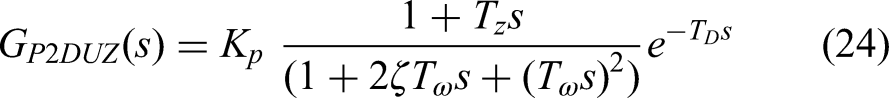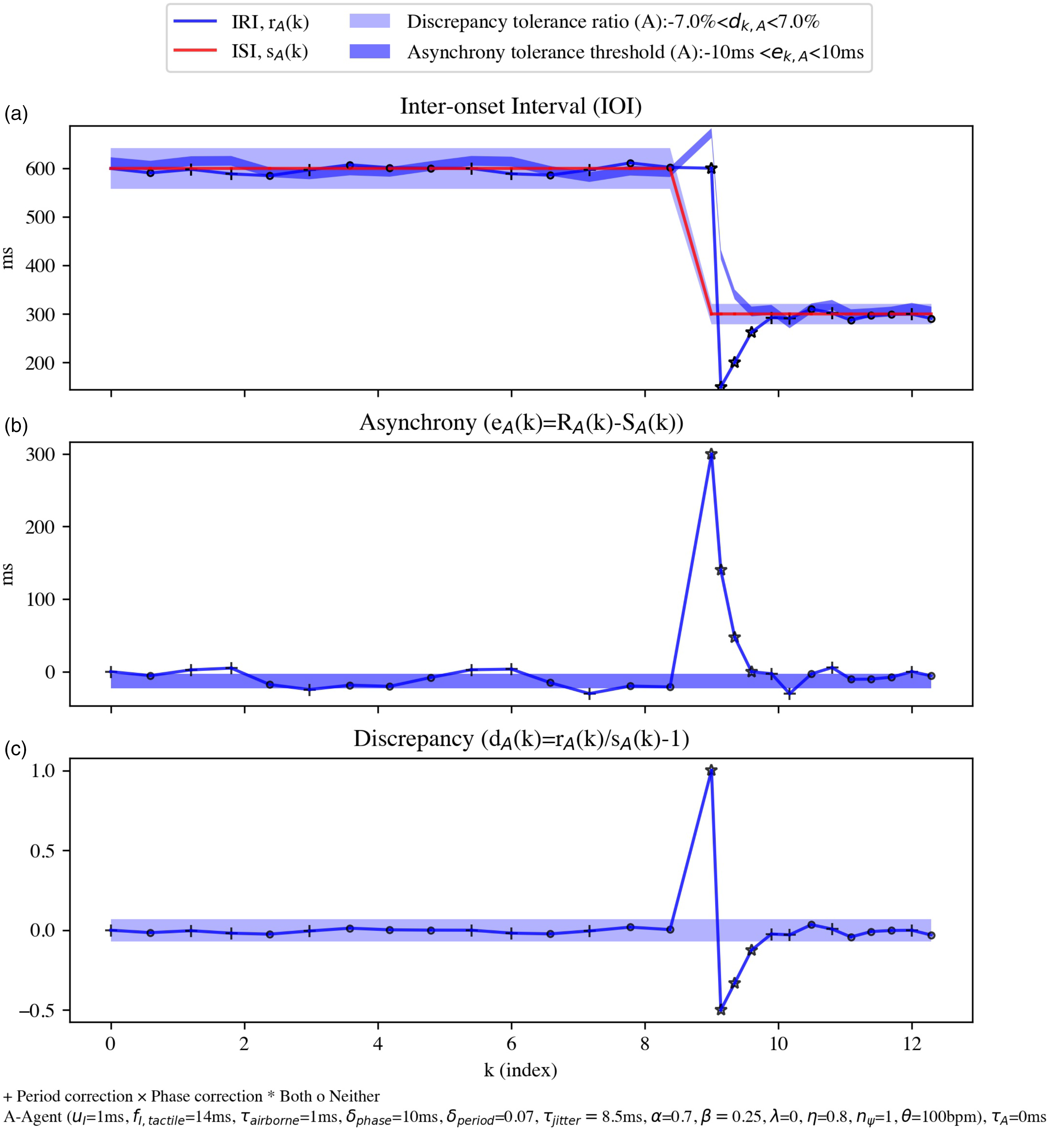The time response to the step change in tempo was modeled by quantifying five parameters presented in the following equations (the gain $K_{p}$ , the delay $T_{D}$ , the first two poles defined by $T_{ω}$ and $ζ$ , and a zero defined by $T_{z}$ ):

G_{P 2 D U Z} (s) = K_{p} \frac{1 + T_{z} s}{(1 + 2 ζ T_{ω} s + {(T_{ω} s)}^{2})} e^{- T_{D} s}

(24)

T_{ω} = \frac{1}{f_{ω}} = \frac{2 π}{ω}

(25)

p_{1, 2} = \frac{- ζ \pm \sqrt{ζ^{2} - 1}}{T_{ω}}

(26)

z = - \frac{1}{T_{z}}

(27)

Figure 10.

Scenario 3: Simulation of tapping an agent against a step-changing metronome, with a tempo jumping from 100 to 140 bpm (that is, IRI from 600 ms to 429 ms), showing (a) IRI and ISI, (b) phase error, and (c) period error. The dark blue area marks the IRI range within which the asynchrony is tolerated (that is, outside of which the phase error correction process is activated, marked by +). The light blue area depicts the tolerance range for period error correction process. Onsets for agent A are marked by × if the latter mechanism is activated. Planned intervals that fall within both light and dark blue ranges are marked by ○ and are not corrected for either process, although they can still be executed with a jitter.

Similar to the experimental data reported by Darabi and Svensson (2021), we chose three randomly generated agents, aggregated and upsampled the simulated trials according to the algorithm described in the original experiment, and compared the results with the aggregated observations from the three human subjects over the same reported step changes and number of repetitions. With forcing the gain $K_{p} = 1$ , the other four parameters, that is, ( $T_{D}, T_{ω}, ζ, T_{z}$ ), are numerically identified for each step size in the range of 102–200 bpm.

Figure 11 shows one example of the 27 analyzed step responses to sudden tempo changes. The positive step change (Figure 11(a)) shows an increase in the interval, in this example, from 429 to 600 ms, equivalent to a decrease in tempo from 140 to 100 bpm, after normalization to a unit step response. Conversely, in line with Figure 10, the negative step change (Figure 11(b)) shows a sudden reduction in the interval or an increase in tempo by the same values. Both charts are normalized by the step size, so the step input ranges between 0 and 1 (or −1). The green curves show the experimental data with the brown curves representing their simulated counterparts. The thicker, lighter curves show the upsampled aggregated step responses for this step size, aggregated over all participants/agents and their repetitions (observed or simulated). The thinner, darker curves show the aggregated step response modeled by a pair of complex poles, a delay, and a zero according to the dynamical systems method in equation (24) (observed or simulated).

Figure 11.

Step response to a sudden tempo change between 100 and 140 bpm. A positive step (a) shows an increase in the interval or a decrease in tempo. Conversely, a negative step (b) shows a reduction in the interval (increase in tempo). Aggregated trials from three participants in a real-world experiment (green) is compared with that of three randomly chosen simulated agents (brown). The thicker lighter curves represent the aggregated IRIs over all participants and repetitions, upsampled with PCHIP interpolation. MATLAB system identification toolbox models the darker, thinner lines with a delay, one zero, and two poles (also known as a P2DUZ model. The accuracy of the model is reported with a fit ratio based on a normalized root-mean-square error (NRMSE).

For subliminal step changes, where the relative change in the tempo is below 7% (Repp, 2001b), the results of the identified parameters are overall noisy, particularly for the experimental data. For the supraliminal step changes in the range of 108 to 200 bpm, we observed similar trends for both observation and simulation, and checked if a linear regression can predict the identified values.

In Figure 12, the top two charts ( $T_{ω}$ and $ζ$ ) determine the position of the first two poles. At minimal steps, where the discrepancy is not large enough to be quickly registered, the period error correction process is not activated. Therefore, a longer time (several taps) is expected for the phase error to be accumulated until it gets corrected by the corresponding process. This explains a larger oscillation period ( $T_{ω})$ across subliminal steps (below 108 bpm) across both simulated (brown) and observed (green) trials. This is in accordance with the experimental observations of longer-lasting overshoots at smaller steps, that is, a higher oscillation period and lower oscillation frequency. At larger steps, where both processes are activated, the immediate awareness of the tempo change causes a faster correction, characterized by a decline in oscillation frequency ( $T_{ω}$ ) for supraliminal steps (at both positive and negative steps, in simulated and experimental data). This decline means that the IRI's frequency of oscillation following the input ISI will increase for larger step sizes.

Figure 12.

Identified model parameters expressed as a function of the relative step size for P2DUZ model (the first two poles, $T_{ω}$ and $ζ$ ; delay, $T_{d}$ ; and the zero, $T_{z}$ ), compares three simulated agents (aggregated) with three human subjects (aggregated). The linear regressions are performed only for datapoints above 7% (steps in the supraliminal regime; 108 ms and above).

The damping ratio ( $ζ$ ) also takes higher values in the subliminal range than in the supraliminal range. We can observe this again for positive and negative steps and across observation and simulation data. Typically, the higher the value of the damping ratio, the smaller the size of the overshoot (Fadali & Visioli, 2012). This trend in supraliminal steps translates to larger overshoots in the step response, even relative to its larger magnitude (the change in the input ISI). In other words, when $r (k)$ follows a step change in $s (k)$ , supraliminal changes exhibit a larger overshoot compared with subliminal changes, not only in absolute terms but also relative to the larger magnitude of the input step. The model fitting, through the estimation of the third parameter ( $T_{d}$ ), detects a stable and minimal latency below 0.1 s for both simulation and experiment and in both directions. Studying the next parameter ( $T_{z}$ ) shows a disagreement in the subliminal range between the simulation and the experiment.

In the supraliminal range, however, there is a good agreement in estimating the zero value between the observation and the simulation, as seen in the good alignments between the linear regressions in each subplot. To summarize, Figure 13 shows the estimated parameters of the experimental data against those calculated from the simulation. The unit on both axes is seconds, except for the damping ratio ( $ζ$ ) which is scalar.

Figure 13.

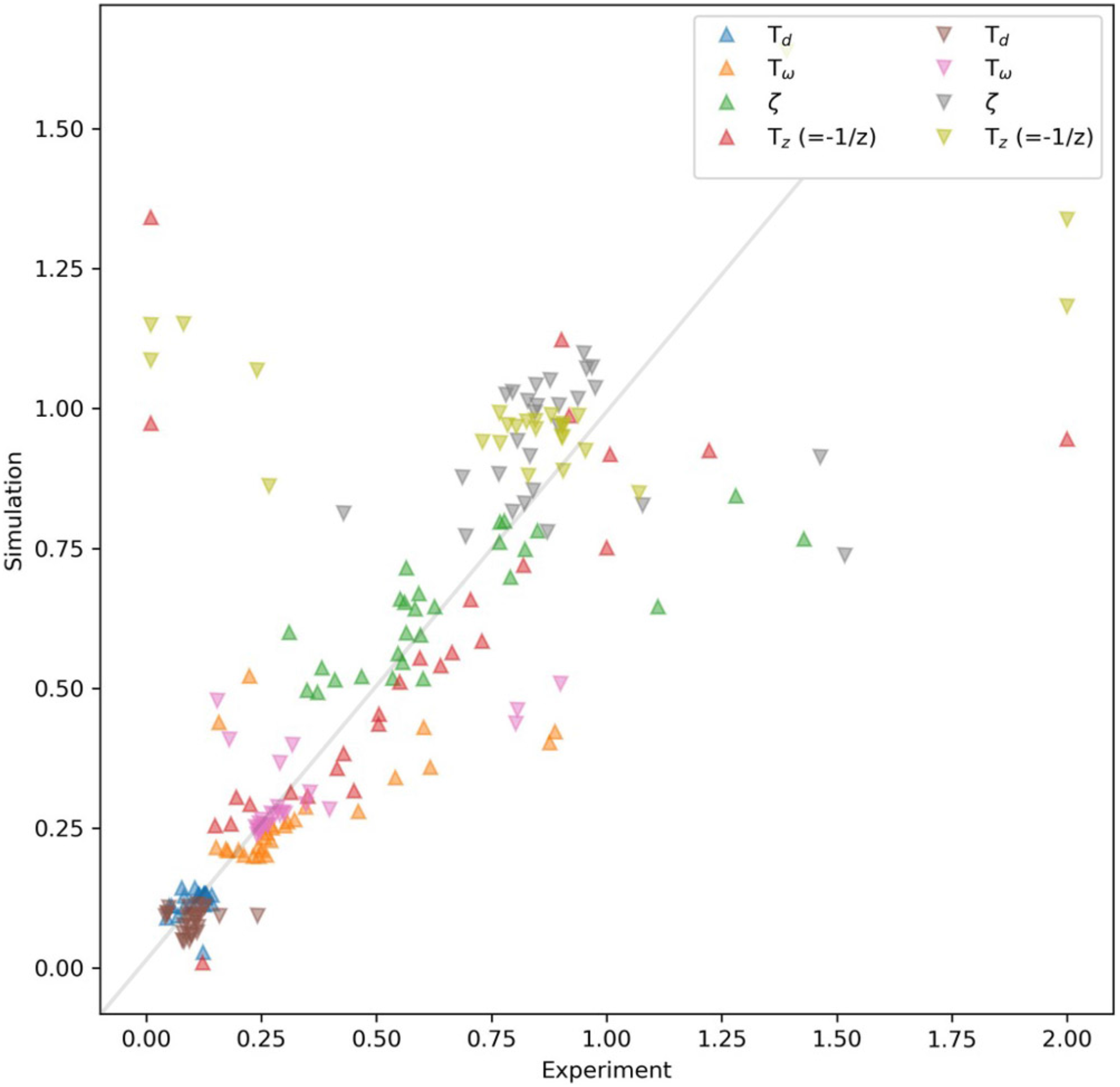
Identified parameters for the experiment versus simulation for the P2DUZ model. The unit on both axis is seconds, except for the damping ratio ( $ζ$ ) which is scalar. Data points with (∧) are from the positive tempo step experiments while those with (∨) data points represent the negative tempo step experiments. Includes diagonal lines.

Another statistical method we use to analyze the agreement between the simulation and the experiment in the time domain is the mean-difference (Altman) plot (Cleveland, 1993). Consider two IRI arrays of the same length, both from the same step size and direction, one from observation and the other from the simulation. Assume $r_{E x p e r i m e n t}$ to be the aggregated data from all repetitions of participants in the experiment and $r_{S i m u l a t i o n}$ to be the array aggregating all repetitions of the simulated agents. This plot can show systematic differences between the two arrays (that is, any fixed bias) by looking into whether their mean difference deviates significantly from 0 in comparison with the standard deviation of the difference. It can also reveal possible outliers that do not cluster around the other data points. Figure 14 shows the mean of the timings of the corresponding onsets between these two arrays against their difference for each direction and each step size, by plotting the Cartesian coordinates of a given sample A as follows:

A (x, y) = A (\frac{r_{E x p e r i m e n t} + r_{S i m u l a t i o n}}{2}, r_{E x p e r i m e n t} - r_{S i m u l a t i o n})

(28)

Figure 14.

Altman plots, showing the agreement between the model outcomes and human performance for scenario 3. The horizontal axis represents the tempo related to the average of corresponding IRIs from the experiment and simulation data (in bpm). The vertical axis shows the time difference between corresponding IRIs of the simulation and the experiment when expressed in terms of tempo (in bpm). The solid horizontal line marks the mean difference between the two arrays. This line does not differ significantly from 0 with respect to the dashed lines (the mean of differences ± 1.96 standard deviation of the difference), also known as the 95% limits of agreement.

In this figure, the horizontal axis shows the average of experiment and simulation, and the vertical axis shows their difference. The solid horizontal line shows the mean difference between the two arrays. This line does not differ significantly from 0 in comparison with the dashed lines which show this mean of differences ± 1.96 standard deviation of the difference, also known as the 95% limits of agreement,⁶ which does not indicate the presence of a systemic bias. If a consistent bias is observed, it can be adjusted for by subtracting the mean difference from the new method.

Conclusion

We have simulated a “rhythmic agent” by deconstructing and modifying the Mates’ behavioral model of SMS. The auditory and tactile components of the tap's feedback were adjustable with a weighting factor. In addition to the adaptive/reactive error correction processes, a mechanism to extrapolate anticipation linearly has been introduced. Period estimation and period correction were both incorporated, as with the application of short-term memory, both were deemed necessary to produce human-like tempo adjustment. The simulation confirmed observed patterns of human synchronization across three scenarios.

In scenario 1, exposing the agent to a simple metronome recreated the well-known human behavioral phenomenon, NMA, that while subjects tap to a metronome, taps tend to precede a sound stimulus onset by a few tens of milliseconds, instead of being distributed symmetrically around the sound onsets. A single parameter $λ$ was used to shift the dominance from tactile to auditory feedback. While in agreement with the Paillard–Fraisse hypothesis (Fraisse, 1980), the entire range of $λ$ produced some NMA, the dependency of the observed effect on the balance between auditory and tactile feedback was examined. We showed that changing the value of $λ$ from 0 (tactile afferent dominance) to 1 (auditory afferent dominance) produces a smaller absolute value for NMA. Alternatively, a lower $λ$ , that is, higher dominance of the tactile afferent feedback of the tap as opposed to the auditory, intensified the NMA.

In scenario 2, the presented model was tested in a joint delayed rhythmic collaboration, and the so-called “Chafe effect” was reproduced. That is, if a communication delay is introduced, the tempo decreases in a similar manner as observed in real-world experiments. In addition, a speed-up effect is observed for transmission delays smaller than around 10 ms.The introduction of jitter in our model generates case-to-case variation similar to real experiments. The weighting factor, $λ$ , affected the degree of speed-up for low delays. A decrease in the value of $λ$ , which in the first scenario increased the NMA, strengthened the Chafe effect by increasing the delay threshold at which trials are stable. It was also shown that including anticipation in addition to the reactive mechanism decreases this effect. It was also concluded that the acceleration at minimal latencies during coordinated joint tapping can be attributed to NMA with the two, in part, having a common neurosensory/biophysical cause.

In scenario 3, an agent performing against a step-changing metronome generated overshoot in its reaction to a tempo step in similar manners as observed in real-world experiments. Fitting a dynamical system model to the simulated data, some modeled parameters of the overshoot, namely $ζ$ and $T_{ω}$ , or the damping ratio and the oscillation frequency of the step response signal, behaved in a similar manner as human adjustment to tempo step changes. In the supraliminal range of tempo changes, similar values and trends of dependency of these parameters on the step size were observed, while the results appeared noisy and not conclusive at the subliminal range.

We can think of two applications for this model. Practically, to implement an automatic musical accompaniment application, the model can be combined with a real-time beat tracking algorithm to dynamically track the location of a received input signal and compare it with a given musical score (Lin et al., 2020). The application would take the role of another instrumentalist or a whole orchestra to accompany the solo musician at the right tempo, with human-like behavior resembling a real-life performance (Arzt, 2016). In addition, the numerical values of the identified parameters of the transfer functions used in the last scenario could inspire SMS models that do not constrain their formulation to the time domain, and eventually inform the value of error correction gains or their formulation.

Footnotes

Action Editor

Jessica Grahn, Western University, Brain and Mind Institute and Department of Psychology.

Peer Review

Jonathan Cannon, McMaster University, Department of Psychology, Neuroscience and Behaviour as well as one anonymous reviewer.

Contributorship

Nima Darabi is the main author who wrote the paper and conducted the experiments. The work is done under U. Peter Svensson's close supervision, and Paul Mertens has provided neurological insights and parts of the literature review while being a part of the pilot research.

Declaration of Conflicting Interests

The authors declared no potential conflicts of interest with respect to the research, authorship, and/or publication of this article.

Ethical Approval

This study is essentially a secondary “analysis,” simulation, or modeling of participant data collected in a previous experiment from three human subjects (e.g., Darabi & Svensson, 2021), which received ethical approval: “The studies involving human participants were reviewed and approved by Q2S Centre of Excellence, NTNU. Written informed consent for participation was not required for this study in accordance with the national legislation and the institutional requirements.”

Funding

The authors disclosed receipt of the following financial support for the research, authorship, and/or publication of this article: This work was supported by the Norges Teknisk-Naturvitenskapelige Universitet, and Uninett through the “Centre for Quantifiable Quality of Service in Communication Systems, Centre of Excellence,” appointed by the Research Council of Norway.

ORCID iDs

Nima Darabi

U. Peter Svensson

Paul Mertens

Data Availability Statement

Data sharing not applicable to this article as no datasets were generated or analyzed during the current study.

Notes

References

Arzt

(2016). Flexible and robust music tracking. Doctoral thesis, Johannes Kepler Universitӓt Linz. http://www.cp.jku.at/research/papers/Arzt_Dissertation.pdf

Aschersleben

(2002). Temporal control of movements in sensorimotor synchronization. Brain and Cognition, 48(1), 66–79. https://doi.org/10.1006/brcg.2001.1304

Aschersleben

(2003). Effects of training on the timing of simple repetitive movements.

Aschersleben

Gehrke

Prinz

(2001). Tapping with peripheral nerve block. Experimental Brain Research, 136(3), 331–339. https://doi.org/10.1007/s002210000562

Aschersleben

Prinz

(1995). Synchronizing actions with events: The role of sensory information. Perception & Psychophysics, 57(3), 305–317. https://doi.org/10.3758/BF03213056

Atkinson

R. C.

Shiffrin

R. M.

(1968). Human memory: A proposed system and its control processes. In Psychology of learning and motivation (Vol. 2, pp. 89–195). Elsevier.

Bååth

Madison

(2012). The subjective difficulty of tapping to a slow beat. 12th International Conference on Music Perception and Cognition, Thessaloniki, Greece.

Babkoff

(1975). Dichotic temporal interactions: Fusion and temporal order. Perception & Psychophysics, 18(4), 267–272. https://doi.org/10.3758/BF03199373

Bartlette

Headlam

Bocko

Velikic

(2006). Effect of network latency on interactive musical performance. Music Perception, 24(1), 49–62. https://doi.org/10.1525/mp.2006.24.1.49

10.

Blumenthal

A. L.

(1975). A reappraisal of Wilhelm Wundt. American Psychologist, 30(11), 1081–1088. https://doi.org/10.1037/0003-066X.30.11.1081

11.

Bose

Byrne

Rinzel

(2019). A neuromechanistic model for rhythmic beat generation. PLoS Computational Biology, 15(5), e1006450. https://doi.org/10.1371/journal.pcbi.1006450

12.

Buhusi

C. V.

Meck

W. H.

(2005). What makes us tick? Functional and neural mechanisms of interval timing. Nature Reviews Neuroscience, 6(10), 755–765. https://doi.org/10.1038/nrn1764

13.

Burnley

Jones

A. M.

(2018). Power–duration relationship: Physiology, fatigue, and the limits of human performance. European Journal of Sport Science, 18(1), 1–12. https://doi.org/10.1080/17461391.2016.1249524

14.

Byrne

Rinzel

Bose

(2020). Order-indeterminant event-based maps for learning a beat. Chaos: An Interdisciplinary Journal of Nonlinear Science, 30(8), 1–13. https://doi.org/10.1063/5.0013771

15.

Byron

T. P.

Fowles

L. C.

(2015). Repetition and recency increases involuntary musical imagery of previously unfamiliar songs. Psychology of Music, 43(3), 375–389. https://doi.org/10.1177/0305735613511506

16.

Chafe

Caceres

J.-P.

Gurevich

(2010). Effect of temporal separation on synchronization in rhythmic performance. Perception, 39(7), 982–992. https://doi.org/10.1068/p6465

17.

Chafe

Gurevich

(2004). Network time delay and ensemble accuracy: Effects of latency, asymmetry. Audio Engineering Society Convention, 117, 6208. https://aes2.org/publications/elibrary-page/?id=12865

18.

Cleveland

(1993). Visualizing data/William S. Cleveland. AT&T Bell Laboratories .

19.

Collyer

C. E.

Boatright-Horowitz

S. S.

Hooper

(1997). A motor timing experiment implemented using a musical instrument digital interface (MIDI) approach. Behavior Research Methods, Instruments, & Computers, 29(3), 346–352. https://doi.org/10.3758/BF03200586

20.

Comstock

D. C.

Balasubramaniam

(2018). Neural responses to perturbations in visual and auditory metronomes during sensorimotor synchronization. Neuropsychologia, 117, 55–66. https://doi.org/10.1016/j.neuropsychologia.2018.05.013

21.

Cullen

J. K.

Ellis

Berlin

Lousteau

(1972). Human acoustic nerve action potential recordings from the tympanic membrane without anesthesia. Acta oto-Laryngologica, 74(1-6), 15–22. https://doi.org/10.3109/00016487209128417

22.

Darabi

Forbord

Svensson

(2010a). Parametric Modeling of Human Response to a Sudden Tempo Change. Audio Engineering Society Convention, 129, 8308. https://aes2.org/publications/elibrary-page/?id=15730

23.

Darabi

Svensson

U. P.

(2021). Dynamic Systems Approach in Sensorimotor Synchronization: Adaptation to Tempo Step-Change. Frontiers in Physiology, 12, 667859. https://doi.org/10.3389/fphys.2021.667859

24.

Darabi

Svensson

U. P.

Chafe

(2010b). Simulating Ensemble Rhythmic Interaction Based on Quantifiable Strategy Functions. Audio Engineering Society Convention, 129, 8292. https://aes2.org/publications/elibrary-page/?id=15714

25.

Darabi

Svensson

Farner

(2008). Quantifying the strategy taken by a pair of ensemble hand-clappers under the influence of delay. Audio Engineering Society Convention, 125, 7567. https://aes2.org/publications/elibrary-page/?id=14719

26.

Drake

Jones

M. R.

Baruch

(2000). The development of rhythmic attending in auditory sequences: Attunement, referent period, focal attending. Cognition, 77(3), 251–288. https://doi.org/10.1016/S0010-0277(00)00106-2

27.

Elliott

M. T.

Wing

A. M.

Welchman

A. E.

(2010). Multisensory cues improve sensorimotor synchronisation. European Journal of Neuroscience, 31(10), 1828–1835. https://doi.org/10.1111/j.1460-9568.2010.07205.x

28.

Etani

Marui

Kawase

Keller

P. E.

(2018). Optimal tempo for groove: Its relation to directions of body movement and Japanese nori. Frontiers in Psychology, 9, 462. https://doi.org/10.3389/fpsyg.2018.00462

29.

Fadali

M. S.

Visioli

(2012). Digital control engineering: analysis and design. Academic Press.

30.

Farner

Solvang

Sæbo

Svensson

(2009). Ensemble hand-clapping experiments under the influence of delay and various acoustic environments. Journal of the Audio Engineering Society, 57(12), 1028–1041. https://aes2.org/publications/elibrary-page/?id=15235

31.

Fink

Ulbrich

Churan

Wittmann

(2006). Stimulus-dependent processing of temporal order. Behavioural Processes, 71(2-3), 344–352. https://doi.org/10.1016/j.beproc.2005.12.007

32.

Fraisse

(1980). Les synchronisations sensori-motrices aux rythmes [The sensorimotor synchronization of rhythms]. In J. Requin (Ed.), Anticipation et comportement, 233–257. Centre National.

33.

Fraisse

(1982). Rhythm and tempo. The Psychology of Music, 1, 149–180. Academic Press. https://doi.org/10.1016/B978-0-12-213562-0.50010-3

34.

Friberg

Sundberg

(1995). Time discrimination in a monotonic, isochronous sequence. The Journal of the Acoustical Society of America, 98(5), 2524–2531. https://doi.org/10.1121/1.413218

35.

Friberg

Sundströöm

(2002). Swing ratios and ensemble timing in jazz performance: Evidence for a common rhythmic pattern. Music Perception, 19(3), 333–349. https://doi.org/10.1525/mp.2002.19.3.333

36.

Fujii

Hirashima

Kudo

Ohtsuki

Nakamura

Oda

(2011). Synchronization error of drum kit playing with a metronome at different tempi by professional drummers. Music Perception: An Interdisciplinary Journal, 28(5), 491–503. https://doi.org/10.1525/mp.2011.28.5.491

37.

Gasser

H. S.

Grundfest

(1939). Axon diameters in relation to the spike dimensions and the conduction velocity in mammalian A fibers. American Journal of Physiology-Legacy Content, 127(2), 393–414. https://doi.org/10.1152/ajplegacy.1939.127.2.393

38.

Goel

Tashakkori

(2015). Correlation between body measurements of different genders and races. In Collaborative mathematics and statistics research (pp. 7–17). Springer.

39.

Hary

Moore

(1987). Synchronizing human movement with an external clock source. Biological Cybernetics, 56(5), 305–311. https://doi.org/10.1007/BF00319511

40.

Hendrich

Strobach

Buss

Mueller

H. J.

Schubert

(2012). Temporal-order judgment of visual and auditory stimuli: Modulations in situations with and without stimulus discrimination. Frontiers in Integrative Neuroscience, 6, 63. https://doi.org/10.3389/fnint.2012.00063

41.

Ivry

(1997). Cerebellar timing systems. International Review of Neurobiology, 41, 555–573. https://doi.org/10.1016/S0074-7742(08)60370-0

42.

Jantzen

Ratcliff

B. R.

Jantzen

M. G.

(2018). Cortical networks for correcting errors in sensorimotor synchronization depend on the direction of asynchrony. Journal of Motor Behavior, 50(3), 235–248. https://doi.org/10.1080/00222895.2017.1327414

43.

Kaernbach

Schr

Muller

Schroger

(2004). Psychophysics beyond sensation: laws and invariants of human cognition. Psychology Press.

44.

Kamal

Yadav

P. K.

(2016). Estimation of stature from different anthropometric measurements in Kori population of North India. Egyptian Journal of Forensic Sciences, 6(4), 468–477. https://doi.org/10.1016/j.ejfs.2016.12.001

45.

Kanabus

Szelag

Rojek

Poppel

(2002). Temporal order judgement for auditory and visual stimuli. Acta Neurobiologiae Experimentalis, 62(4), 263–270. https://doi.org/10.55782/ane-2002-1443

46.

Keller

P. E.

Novembre

Hove

M. J.

(2014). Rhythm in joint action: Psychological and neurophysiological mechanisms for real-time interpersonal coordination. Philosophical Transactions of the Royal Society B: Biological Sciences, 369(1658), 20130394. https://doi.org/10.1098/rstb.2013.0394

47.

Krause

Schnitzler

Pollok

(2010). Functional network interactions during sensorimotor synchronization in musicians and non-musicians. NeuroImage, 52(1), 245–251. https://doi.org/10.1016/j.neuroimage.2010.03.081

48.

Kruger

Michel

(1962). Reinterpretation of the representation of pain based on physiological excitation of single neurons in the trigeminal sensory complex. Experimental Neurology, 5(2), 157–178. https://doi.org/10.1016/0014-4886(62)90031-6

49.

Large

E. W.

(2008). Resonating to musical rhythm: Theory and experiment. The Psychology of Time (ed. S Grondin), 189–232. Bingley, UK: Emerald Group Publshing. https://dx.doi.org/10.1016/B978-0-08046-977-5.00006-5

50.

Large

E. W.

Roman

Kim

J. C.

Cannon

Pazdera

J. K.

Trainor

L. J.

Rinzel

Bose

(2023). Dynamic models for musical rhythm perception and coordination. Frontiers in Computational Neuroscience, 17, 1151895. https://doi.org/10.3389/fncom.2023.1151895

51.

Lauzon

A. P.

Russo

F. A.

Harris

L. R.

(2020). The influence of rhythm on detection of auditory and vibrotactile asynchrony. Experimental Brain Research, 238(4), 825–832. https://doi.org/10.1007/s00221-019-05720-x

52.

Lieberman

Sohmer

Szabo

(1973). Standard values of amplitude and latency of cochlear audiometry (electro-cochleography) responses in different age groups. Archiv für klinische und experimentelle Ohren-, Nasen-und Kehlkopfheilkunde, 203(4), 267–273. https://doi.org/10.1007/BF00316802

53.

Lin

Y.-J.

Kao

H.-K.

Tseng

Y.-C.

Tsai

(2020). A Human-Computer Duet System for Music Performance. Proceedings of the 28th ACM International Conference on Multimedia.

54.

Ljung

(1999). System identification. Wiley encyclopedia of electrical and electronics engineering. https://doi.org/10.1002/047134608x.w1046.

55.

Loehr

J. D.

Large

E. W.

Palmer

(2011). Temporal coordination and adaptation to rate change in music performance. Journal of Experimental Psychology: Human Perception and Performance, 37(4), 1292. https://doi.org/10.1037/a0023102

56.

Loewenstein

W. R.

Rathkamp

With the Assistance of Zamudio

(1958). The sites for mechano-electric conversion in a Pacinian corpuscle. The Journal of General Physiology, 41(6), 1245–1265. https://doi.org/10.1085/jgp.41.6.1245

57.

Z.-L.

Sperling

(2003). Measuring sensory memory: Magnetoencephalography habituation and psychophysics. In Magnetic source imaging of the human brain (pp. 319–342). Psychology Press.

58.

Madison

Merker

(2002). On the limits of anisochrony in pulse attribution. Psychological Research, 66(3), 201–207. https://doi.org/10.1007/s00426-001-0085-y

59.

Margolis

R. H.

Levine

S. C.

Foamier

E. M.

Hunter

L. L.

Smith

S. L.

Lilly

D. J.

(1992). Tympanic electrocochleography: Normal and abnormal patterns of response. International Journal of Audiology, 31(1), 8–24. https://doi.org/10.3109/00206099209072898

60.

Mates

(1994a). A model of synchronization of motor acts to a stimulus sequence. I. Timing and error corrections. Biological Cybernetics, 70(5), 463–473. doi: https://doi.org/10.1007/BF00203239

61.

Mates

(1994b). A model of synchronization of motor acts to a stimulus sequence. II. Stability analysis, error estimation and simulations. Biological Cybernetics, 70(5), 475–484. https://doi.org/10.1007/BF00203240

62.

Mates

Aschersleben

(2000). Sensorimotor synchronization: The impact of temporally displaced auditory feedback. Acta Psychologica, 104(1), 29–44. https://doi.org/10.1016/S0001-6918(99)00052-9

63.

McAuley

J. D.

Jones

M. R.

Holub

Johnston

H. M.

Miller

N. S.

(2006). The time of our lives: Life span development of timing and event tracking. Journal of Experimental Psychology: General, 135(3), 348–367. https://doi.org/10.1037/0096-3445.135.3.348

64.

Michon

(1967). Timing in temporal tracking. Van Gorcum/Inst. For Perception RVO-TNO.

65.

Mills

P. F.

Harry

Stevens

C. J.

Knoblich

Keller

P. E.

(2019). Intentionality of a co-actor influences sensorimotor synchronisation with a virtual partner. Quarterly Journal of Experimental Psychology, 72(6), 1478–1492. https://doi.org/10.1177/1747021818796183

66.

Mills

P. F.

van der Steen

M. M.

Schultz

B. G.

Keller

P. E.

(2015). Individual differences in temporal anticipation and adaptation during sensorimotor synchronization. Timing & Time Perception, 3(1-2), 13–31. https://doi.org/10.1163/22134468-03002040

67.

Miyake

(1901). Researches on rhythmic action. Yale University.

68.

Norris

A. H.

Shock

Wagman

(1953). Age changes in the maximum conduction velocity of motor fibers of human ulnar nerves. Journal of Applied Physiology, 5(10), 589–593. https://doi.org/10.1152/jappl.1953.5.10.589

69.

Nowicki

Prinz

Grosjean

Repp

B. H.

Keller

P. E.

(2013). Mutual adaptive timing in interpersonal action coordination. Psychomusicology: Music, Mind, and Brain, 23(1), 6–20. https://doi.org/10.1037/a0032039

70.

Nozaradan

Keller

P. E.

Rossion

Mouraux

(2018). EEG frequency-tagging and input–output comparison in rhythm perception. Brain Topography, 31(2), 153–160. https://doi.org/10.1007/s10548-017-0605-8

71.

Pathak

Pucha

Zhang

Y. C.

Mao

Z. M.

(2008). A measurement study of internet delay asymmetry. International Conference on Passive and Active Network Measurement.

72.

Perl

E. R.

Kruger

(1996). Nociception and pain: Evolution of concepts and observations. In Pain and touch (pp. 179–211). Elsevier.

73.

Peters

(1989). The relationship between variability of intertap intervals and interval duration. Psychological Research, 51(1), 38–42. https://doi.org/10.1007/BF00309274

74.

Picton

T. W.

Hillyard

S. A.

Krausz

H. I.

Galambos

(1974). Human auditory evoked potentials. I: Evaluation of components. Electroencephalography and Clinical Neurophysiology, 36(2), 179–190. https://doi.org/10.1016/0013-4694(74)90155-2 .

75.

Pöppel

Schill

von Steinbüchel

(1990). Sensory integration within temporally neutral systems states: A hypothesis. Naturwissenschaften, 77(2), 89–91. https://doi.org/10.1007/BF01131783

76.

Pratt

Sohmer

(1976). Intensity and rate functions of cochlear and brainstem evoked responses to click stimuli in man. Archives of oto-Rhino-Laryngology, 212(2), 85–92. https://doi.org/10.1007/BF00454268

77.

Pressing

Jolley-Rogers

(1997). Spectral properties of human cognition and skill. Biological Cybernetics, 76(5), 339–347. https://doi.org/10.1007/s004220050347

78.

Repp

B. H.

(2001a). Phase correction, phase resetting, and phase shifts after subliminal timing perturbations in sensorimotor synchronization. Journal of Experimental Psychology: Human Perception and Performance, 27(3), 600. https://doi.org/10.1037/0096-1523.27.3.600

79.

Repp

B. H.

(2001b). Processes underlying adaptation to tempo changes in sensorimotor synchronization. Human Movement Science, 20(3), 277–312. https://doi.org/10.1016/S0167-9457(01)00049-5

80.

Repp

B. H.

(2005). Sensorimotor synchronization: A review of the tapping literature. Psychonomic Bulletin & Review, 12(6), 969–992. https://doi.org/10.3758/BF03206433

81.

Repp

B. H.

(2006). Rate limits of sensorimotor synchronization. Advances in Cognitive Psychology, 2(2-3), 163–181. https://doi.org/10.2478/v10053-008-0053-9

82.

Repp

B. H.

(2008). Perfect phase correction in synchronization with slow auditory sequences. Journal of Motor Behavior, 40(5), 363–367. https://doi.org/10.3200/JMBR.40.5.363-367

83.

Repp

B. H.

(2011). Tapping in synchrony with a perturbed metronome: The phase correction response to small and large phase shifts as a function of tempo. Journal of Motor Behavior, 43(3), 213–227. https://doi.org/10.1080/00222895.2011.561377

84.

Repp

B. H.

Doggett

(2007). Tapping to a very slow beat: A comparison of musicians and nonmusicians. Music Perception, 24(4), 367–376. https://doi.org/10.1525/mp.2007.24.4.367

85.

Repp

B. H.

Keller

P. E.

(2004). Adaptation to tempo changes in sensorimotor synchronization: Effects of intention, attention, and awareness. Quarterly Journal of Experimental Psychology Section A, 57(3), 499–521. https://doi.org/10.1080/02724980343000369

86.

Repp

B. H.

Keller

P. E.

(2008). Sensorimotor synchronization with adaptively timed sequences. Human Movement Science, 27(3), 423–456. https://doi.org/10.1016/j.humov.2008.02.016

87.

Repp

B. H.

Keller

P. E.

Jacoby

(2012). Quantifying phase correction in sensorimotor synchronization: Empirical comparison of three paradigms. Acta Psychologica, 139(2), 281–290. https://doi.org/10.1016/j.actpsy.2011.11.002

88.

Repp

B. H.

Penel

(2002). Auditory dominance in temporal processing: New evidence from synchronization with simultaneous visual and auditory sequences. Journal of Experimental Psychology: Human Perception and Performance, 28(5), 1085. https://doi.org/10.1037/0096-1523.28.5.1085

89.

Repp

B. H.

Y. H.

(2013). Sensorimotor synchronization: A review of recent research (2006-2012). Psychonomic Bulletin & Review, 20(3), 403–452. https://doi.org/10.3758/s13423-012-0371-2

90.

Roman

I. R.

Roman

A. S.

Kim

J. C.

Large

E. W.

(2023). Hebbian learning with elasticity explains how the spontaneous motor tempo affects music performance synchronization. PLoS Computational Biology, 19(6), e1011154. https://doi.org/10.1371/journal.pcbi.1011154

91.

Roman

I. R.

Washburn

Large

E. W.

Chafe

Fujioka

(2019). Delayed feedback embedded in perception-action coordination cycles results in anticipation behavior during synchronized rhythmic action: A dynamical systems approach. PLoS Computational Biology, 15(10), e1007371. https://doi.org/10.1371/journal.pcbi.1007371

92.

Rorden

Karnath

H.-O.

(2018). Biased temporal order judgments in chronic neglect influenced by trunk position. Cortex, 99, 273–280. https://doi.org/10.1016/j.cortex.2017.12.008

93.

Sambo

Torta

Gallace

Liang

Moseley

G. L.

Iannetti

(2013). The temporal order judgement of tactile and nociceptive stimuli is impaired by crossing the hands over the body midline. Pain, 154(2), 242–247. https://doi.org/10.1016/j.pain.2012.10.010

94.

Schubotz

R. I.

(2007). Prediction of external events with our motor system: Towards a new framework. Trends in Cognitive Sciences, 11(5), 211–218. https://doi.org/10.1016/j.tics.2007.02.006

95.

Schultz

B. G.

Brown

R. M.

Kotz

S. A.

(2021). Dynamic acoustic salience evokes motor responses. Cortex, 134, 320–332. https://doi.org/10.1016/j.cortex.2020.10.019

96.

Schultz

B. G.

Palmer

(2019). The roles of musical expertise and sensory feedback in beat keeping and joint action. Psychological Research, 83(3), 419–431. https://doi.org/10.1007/s00426-019-01156-8

97.

Schulze

H.-H.

Cordes

Vorberg

(2005). Keeping synchrony while tempo changes: Accelerando and ritardando. Music Perception, 22(3), 461–477. https://doi.org/10.1525/mp.2005.22.3.461

98.

Schwartze

Keller

P. E.

Patel

A. D.

Kotz

S. A.

(2011). The impact of basal ganglia lesions on sensorimotor synchronization, spontaneous motor tempo, and the detection of tempo changes. Behavioural Brain Research, 216(2), 685–691. https://doi.org/10.1016/j.bbr.2010.09.015

99.

Shepard

R. N.

Teghtsoonian

(1961). Retention of information under conditions approaching a steady state. Journal of Experimental Psychology, 62(3), 302–309. https://doi.org/10.1037/h0048606

100.

Stephen

D. G.

Stepp

Dixon

J. A.

Turvey

(2008). Strong anticipation: Sensitivity to long-range correlations in synchronization behavior. Physica A: Statistical Mechanics and its Applications, 387(21), 5271–5278. https://doi.org/10.1016/j.physa.2008.05.015

101.

Stepp

Turvey

M. T.

(2010). On strong anticipation. Cognitive Systems Research, 11(2), 148–164. https://doi.org/10.1016/j.cogsys.2009.03.003

102.

Thaut

M. H.

Stephan

K. M.

Wunderlich

Schicks

Tellmann

Herzog

McIntosh

G. C.

Seitz

R. J.

Hömberg

(2009). Distinct cortico-cerebellar activations in rhythmic auditory motor synchronization. Cortex, 45(1), 44–53. https://doi.org/10.1016/j.cortex.2007.09.009

103.

Tomyta

Ohira

Katahira

(2023). Asymmetric error correction in the synchronization tapping task. Timing & Time Perception, 1(aop), 1–10. https://doi.org/10.1163/22134468-bja10090

104.

Tranchant

Scholler

Palmer

(2022). Endogenous rhythms influence musicians’ and non-musicians’ interpersonal synchrony. Scientific Reports, 12(1), 12973. https://doi.org/10.1038/s41598-022-16686-2

105.

Trojaborg

(1964). Motor nerve conduction velocities in normal subjects with particular reference to the conduction in proximal and distal segments of median and ulnar nerve. Electroencephalography and Clinical Neurophysiology, 17(3), 314–321. https://doi.org/10.1016/0013-4694(64)90132-4

106.

Turgeon

Wing

A. M.

Taylor

L. W.

(2011). Timing and aging: Slowing of fastest regular tapping rate with preserved timing error detection and correction. Psychology and Aging, 26(1), 150–161. https://doi.org/10.1037/a0020606

107.

Van Der Steen

M. C.

Keller

P. E.

(2013). The ADaptation and Anticipation Model (ADAM) of sensorimotor synchronization. Frontiers in Human Neuroscience, 7, 253. https://doi.org/10.3389/fnhum.2013.00253

108.

Vorberg

Schulze

H.-H.

(2002). Linear phase-correction in synchronization: Predictions, parameter estimation, and simulations. Journal of Mathematical Psychology, 46(1), 56–87. https://doi.org/10.1006/jmps.2001.1375

109.

Vorberg

Wing

(1996). Modeling variability and dependence in timing. In Handbook of perception and action (Vol. 2, pp. 181–262). Elsevier.

110.

Vos

P. G.

Helsper

E. L.

(1992). Tracking simple rhythms: On-beat versus off-beat performance. In Time, action and cognition (pp. 287–299). Springer.

111.

Widder

D. V.

(2015). Laplace transform (PMS-6). Princeton university press. https://doi.org/10.1515/9781400876457.

112.

Wing

A. M.

Kristofferson

A. B.

(1973). Response delays and the timing of discrete motor responses. Perception & Psychophysics, 14(1), 5–12. https://doi.org/10.3758/BF03198607

113.

Wohlschläger

(1999). Synchronization error: an error in time perception. Abstracts of the Psychonomic Society.

114.

Wolf

Sebanz

Knoblich

(2018). Joint action coordination in expert-novice pairs: Can experts predict novices’ suboptimal timing? Cognition, 178, 103–108. https://doi.org/10.1016/j.cognition.2018.05.012

115.

Wolpert

D. M.

Ghahramani

Jordan

M. I.

(1995). An internal model for sensorimotor integration. Science, 269(5232), 1880–1882. https://doi.org/10.1126/science.7569931

116.

Wolpert

D. M.

Kawato

(1998). Multiple paired forward and inverse models for motor control. Neural Networks, 11(7-8), 1317–1329. https://doi.org/10.1016/S0893-6080(98)00066-5

117.

Woodrow

(1932). The effect of rate of sequence upon the accuracy of synchronization. Journal of Experimental Psychology, 15(4), 357–379. https://doi.org/10.1037/h0071256

118.

Yang

Ouyang

Holm

Huang

Gan

Zhou

Chao

Wang

Zhang

(2019). A mechanism of timing variability underlying the association between the mean and SD of asynchrony. Human Movement Science, 67, 102500. https://doi.org/10.1016/j.humov.2019.102500

119.

Yang

Ouyang

Holm

Huang

Gan

Zhou

Chao

Wang

Zhang

(2020). Tapping ahead of time: Its association with timing variability. Psychological Research, 84(2), 343–351. https://doi.org/10.1007/s00426-018-1043-2

120.

Zamm

Pfordresher

P. Q.

Palmer

(2015). Temporal coordination in joint music performance: Effects of endogenous rhythms and auditory feedback. Experimental Brain Research, 233(2), 607–615. https://doi.org/10.1007/s00221-014-4140-5

121.

Zamm

Wellman

Palmer

(2016). Endogenous rhythms influence interpersonal synchrony. Journal of Experimental Psychology: Human Perception and Performance, 42(5), 611. https://doi.org/10.1037/xhp0000201

122.

Zemlianova

Bose

Rinzel

(2022). A biophysical counting mechanism for keeping time. Biological Cybernetics, 116(2),205–218. https://doi.org/10.1007/s00422-021-00915-4

Neurologically Motivated Simulation of Ensemble Performance

Abstract

Introduction

The Model

Description of the Variables

The Internal Representation of the External Events

Initiation of the Next Motor Command

Central Interval

Short-Term Memory

Calculating the Planned Interval

Phase Error and its Correction

Period Error and its Correction

Combining Dual Correction Processes

Anticipation

Real-World Range of Intervals

Human Rate Limits to Intervals

Lower Limit

Upper Limit

Simulating Duets

Implementation and Results

Scenario 1: Human Against a Metronome

Scenario 2: Delayed Joint Action

Scenario 3: Agent Versus Step-Changing Metronome

Conclusion

Footnotes

Action Editor

Peer Review

Contributorship

Declaration of Conflicting Interests

Ethical Approval

Funding

ORCID iDs

Data Availability Statement

Notes

References