Sage Journals: Discover world-class research

Abstract

I use household panel data to study the dynamics of relative poverty in China, Germany, the United Kingdom, and the United States. Compared to the three Western countries, not only is relative poverty more common in China, it is also deeper and more severe. Transient poverty accounts for less than half of the total poverty in Germany or the US, but about two-thirds of that in China or the UK. Over three waves, 87% of Germans, 78% of Britons, 71% of Americans, but only 46% of Chinese were never poor. Using a multinomial logistic regression model, the determinants of poverty are found to be very similar across the four countries. But the variance explained by that model is much smaller for China than for the three Western countries. The findings of this paper also challenge some existing understanding of poverty dynamics in general.

Keywords

Relative poverty longitudinal data cross-national comparison China

Introduction

China has a very impressive record of poverty reduction. Using the $1-a-day poverty line, 65% of the Chinese population were poor in 1981. This dropped to 10% in 2004, meaning that half a billion people were lifted out of poverty (World Bank, 2009). And since “the absolute number of poor in the developing world as a whole declined from 1.5 to 1.0 billion over the same period …but for China there would have been no decline in the numbers of poor in the developing world over the last two decades of the 20th century” (World Bank, 2009: iii).

Against the backdrop of this clear policy achievement, there is much about poverty in China that is not well understood. This paper contributes to research in this field in three ways. First, existing research is mainly concerned with absolute poverty. This was quite appropriate when China was a very poor country. But after four decades of sustained economic growth, “extreme poverty, in the sense of not being able to meet the most elementary food and clothing needs, has almost been eliminated in China” (World Bank, 2009: iv). Given this, I focus on relative poverty in this paper.

Secondly, previous studies mostly draw on repeated cross-sectional data (for exceptions, see Jalan and Ravallion, 1998, 2000). Although they are very informative about the aggregate poverty trend, they are also silent on the poverty dynamics of individuals. To elaborate, suppose that half of the population were found to be poor on two occasions. This pattern of no overall change might have arisen because everyone's poverty status was stable over time. Alternatively, everyone's poverty status might have changed: those who were poor initially had become non-poor, and vice versa. The welfare implications of these two scenarios and the policy interventions that they call for are quite different (Atkinson, 2019: 63). To determine the poverty dynamics of individuals, I analyse household panel data in this paper.

Thirdly, I carry out parallel analyses for China, Germany, the United Kingdom, and the United States. Large-scale and nationally representative household panel data are hard to come by. Consequently, there are just a few papers that compare poverty dynamics across countries; and they all have a Western focus (Duncan et al., 1993; Fouarge and Layte, 2005; Layte and Whelan, 2003; Valletta, 2006). As high-quality Chinese household panel data have recently become available, I am able to compare China with three Western countries that are very prominent in the relative poverty literature, namely Germany, the UK, and the US. As it turns out, this comparison brings out just how distinctive the Chinese case is. It also revises some of our understanding of poverty dynamics in general.

The rest of this paper is structured as follows. In the second section, I review past research on absolute poverty in China and also research on poverty dynamics in Western societies. The third section introduces the data sets and explains the key operational decisions that I have made. The fourth section reports the results in six parts. Finally, in the fifth section, I summarise the results and discuss their implications for understanding both poverty in China and the dynamics of relative poverty in general.

Context and previous research

Absolute poverty in China

Scholars, government agencies and international organisations have used different poverty lines in their research. So, there is a range of estimates of the level of poverty in China (see e.g., Li et al., 2013: 74, Table 2.16). But all studies point to a large decline over the past 40 years, irrespective of which poverty line is used (Ravallion and Chen, 2007; Zhang et al., 2014).

Appleton et al. (2010) argue that the main driver of poverty reduction in China is economic growth, not redistribution or anti-poverty programmes. And since absolute poverty in China is “predominantly a rural phenomenon” (Gustafsson and Zhong, 2000: 984), it was “[g]rowth in the primary sector (primarily agriculture) [that] did more to reduce poverty” (Ravallion and Chen, 2007: 2). The critical policy change that spurred rural growth in the 1980s was the decollectivisation of agriculture and the return to family farming (Oi, 1989).

It is well-known that income inequality in China has risen very sharply since the mid-1980s (Chan et al., 2019; Xie and Zhou, 2014). It might be thought that a higher level of inequality is the necessary price to pay for the economic growth that is needed to reduce poverty. But there is no evidence for this. As Ravallion and Chen (2007: 3) observe, “[t]he periods of more rapid growth did not bring more rapid increase in inequality. Nor did provinces with more rapid rural income growth experience a steeper increase in inequality. Thus, provinces that saw a more rapid rise in inequality saw less progress against poverty, not more”.

The progress in poverty reduction was uneven, with “[h]alf of the decline in the number of poor came in the first half of the 1980s” (Ravallion and Chen, 2007: 2). After the mid-1980s, the poverty headcount continued to fall, but there were reverses and the rate of decline slowed down considerably. Spatially speaking, there is more poverty in Western China than in the central provinces which, in turn, are poorer than the provinces on the Eastern coast (Gustafsson and Sai, 2009). Li et al. (2013: 76) observe that “[b]y all measures, China's poor is heavily concentrated in the West”.

Of even greater importance than the regional difference is the urban–rural divide. Ravallion and Chen (2007: 8) show that “[f]or all years and all measures, rural poverty incidence exceeds urban poverty and by a wide margin”. Similarly, Li et al. (2013: 75) report that “[u]sing absolute poverty measures, more than 95 percent of the poor were rural”.

The concentration of poverty in rural areas is a direct consequence of the pre-reform strategy of fuelling industrialisation by squeezing the countryside (Oi, 1989). Before the market reform, urbanites enjoyed secure employment and a wide range of benefits and services that were provided through their work units (danwei). Although meagre by Western standards, income and consumption were far higher in Chinese cities than in the countryside.

This created a strong incentive for peasants to move to the cities. To restrict rural–urban migration, a system of household registration (hukou) was introduced in the 1950s which has for decades “effectively bound peasants to the soil” (Whyte, 2005: 10). Restriction on migration has gradually been relaxed and there are now over 200 million internal migrants in China (Liang et al., 2014). But hukou still exists as a legal category. Migrant workers living in cities do not have access to health care, education, or other public services that are available to those with urban hukou (Chan and Zhang, 1999). Furthermore, as migrants tend to work in unskilled, low-wage jobs, they are typically found at the bottom of the urban economic hierarchy.

Despite that, the impact of migration on urban poverty seems quite small. Park and Wang (2010) show that in terms of housing conditions and other non-monetary welfare indicators migrants are indeed worse off than non-migrants. Migrants also earn lower hourly wages. But as they tend to work longer hours and have a lower dependency ratio in their household, the gap in disposable income between migrant and non-migrant households is smaller than might be expected. Overall, Park and Wang (2010: 55) conclude that the difference in poverty rate among migrants and non-migrants is very small and that “including migrants has a negligible impact on the overall urban poverty estimates”.

In the countryside, remittances from migrants certainly help raise household income. But Du et al. (2005: 706) point out that “[t]he poorest rural households with few laborers and poor human capital are unable to allow members to migrate”. Thus, “the overall impact of migration on [rural] poverty headcount has been modest”.

Although poverty in China is concentrated in the countryside, urban Chinese have been facing greater poverty risks since the mid-1990s. In particular, state-owned enterprise (SOE) reforms had led to 28 million workers (about a quarter of the SOE workforce) being laid off (Appleton et al., 2014). This contributed to the doubling of the urban unemployment rate from 6% to 12% between 1993 and 2000 (Meng and Gregory, 2007).

Other reforms also put economic pressure on city dwellers. In particular, the Chinese state used to subsidise urbanites’ food consumption through a coupon system. The value of the coupons distributed to each household was a function of its size and the age of its members. The coupon system was abolished in 1993 and food price control was lifted. Although urban wages had gone up, giving urbanites greater spending power to cope with food price inflation, larger households with few working members lost out in this reform (Meng and Gregory, 2007). Also, urbanites now need to pay for many public services, for example, education and health care, that were previously free or heavily subsidised.

In response to the growing economic hardship in the cities, the Chinese state piloted a minimum living standard guarantee programme (dibao) in Shanghai in 1993, which was then rolled out across urban China in 1999. In 1999, 2.7 million urbanites were enrolled on dibao, rising to 23.4 million in 2008 (Gustafsson and Deng, 2011). A dibao programme for rural China was launched later and became nationwide in 2007. By 2012, it covered 53 million people, about 8% of the rural population (Li and Sicular, 2014).

As with many social programmes in China, the implementation of dibao is very decentralised. Municipal and provincial authorities have a lot of leeway in setting the dibao line, determining the eligibility criteria, and so on (Ravallion, 2014). The World Bank (2009: 123–124) reports that in 2004 the income threshold for rural dibao ranges between 120 yuan and 1560 yuan per person per year. In any case, due to the restricted coverage of the dibao programmes, their impact on poverty reduction is limited (Chen et al., 2006; Li and Sicular, 2014). Overall, a good deal is known about absolute poverty in China. But, as I will show below, relative poverty is a different story altogether.

Cross-national research on relative poverty dynamics

There are only a few cross-national comparative papers on the dynamics of relative poverty. Layte and Whelan (2003) and Fouarge and Layte (2005) analyse panel data from 11 countries that took part in the European Community Household Panel.¹ They show that “the pattern of poverty persistence is congruent with welfare regime theory” (Layte and Whelan, 2003: 167), with “social democratic regimes reducing the level of persistent and recurrent poverty. Liberal and Southern European regime countries have both higher rates and longer duration of poverty” (Fouarge and Layte, 2005: 407).

With a more microscopic lens, Duncan et al. (1993) analyse panel data from Canada, France, Germany, Ireland, Luxembourg, the Netherlands, Sweden and the US. They make several observations that are especially relevant to this paper. First, if the relative poverty line is defined with reference to each country's median income, “the resulting poverty estimates reflect the degree of inequality of the distribution of size-adjusted family income” (Duncan et al., 1993: 217). That is to say, relative poverty tends to be higher in countries with greater income inequality (see also Atkinson, 2015: 25–26).

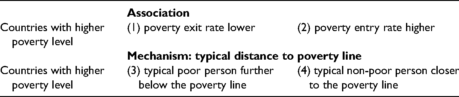
Secondly, there are “striking [cross-national] differences in the prevalence of transitions out of poverty …Countries with larger fractions of their populations below the poverty line have lower escape rates” (Duncan et al., 1993: 221). Escape rates also depend on how far below the poverty line the typical poor person is, “[s]ince crossing a poverty line is generally easiest when a family's income is close to the line” (Duncan et al., 1993: 218). Thus, for example, Duncan et al. (1993: Tables 1 and 2) show that, compared to their European counterparts, the poor in America (especially African American poor) are further away from the poverty line, and their escape rate is, correspondingly, the lowest of all in the sample.

Table 1.

Summary of the observations by Duncan et al. (1993) of cross-national association between relative poverty level and poverty entry and exit rates (top panel), and the mechanism mediating these associations (bottom panel).

	Association
Countries with higher poverty level	(1) poverty exit rate lower	(2) poverty entry rate higher
	Mechanism: typical distance to poverty line
Countries with higher poverty level	(3) typical poor person further below the poverty line	(4) typical non-poor person closer to the poverty line

Table 2.

Poverty line (60%-of-median-income) of the four countries at wave 1 in local currency and purchasing power parity (PPP) dollar.

	Local currency	PPP $
Germany	€ 12,067	14,879
United Kingdom	£ 10,350	14,744
United States	$ 17,789	17,789
China	¥ 7275	2199
China (urban)	¥ 9546	2886
China (rural)	¥ 5576	1686

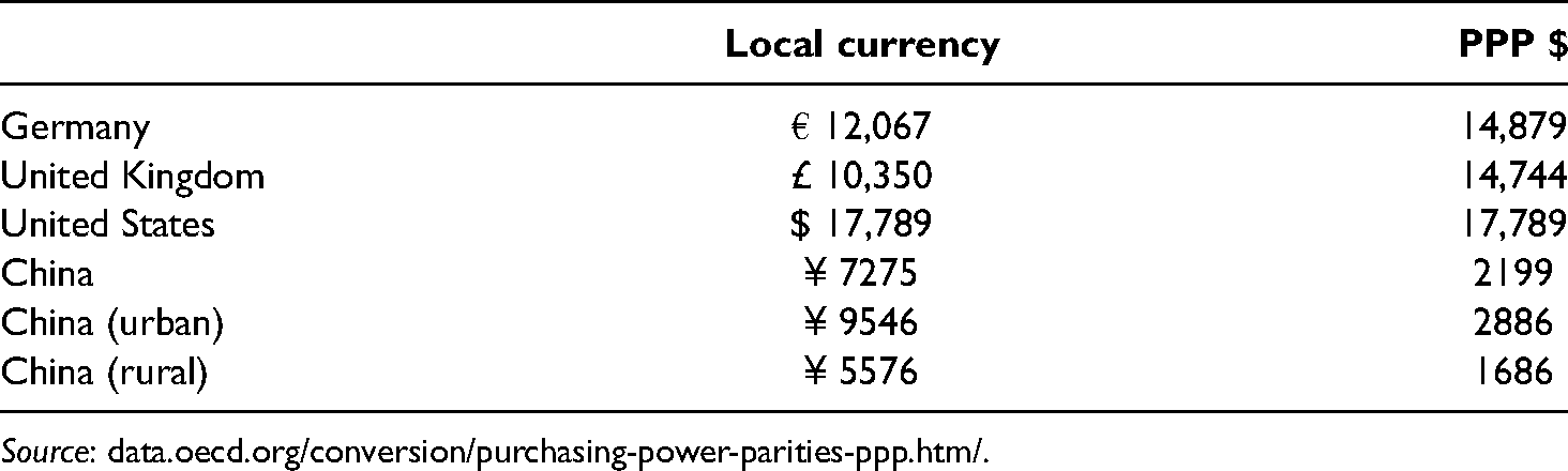
Source: data.oecd.org/conversion/purchasing-power-parities-ppp.htm/.

Thirdly, Duncan et al. (1993: 224–225) report “a decidedly inverse relationship between the fraction of the population at risk of entering poverty and the fraction who actually fall below the line”. Put differently, poverty entry rates are lower in countries with less relative poverty. They offer a similar explanation for this association: “the greater the fraction of the population above poverty, the greater is the likely distance between the typical nonpoor family and the poverty threshold and the less likely that family is to make the transition” (Duncan et al., 1993: 225). Table 1 summarises these suggested associations and mechanisms (see also Jäntti and Danziger, 2000: 355–358). As I will show below, the cross-national comparative analyses of this paper suggests that some revisions to the second and third claims above are necessary.

Data

The data that I analyse are collected in four household panel surveys, namely the China Family Panel Studies (CFPS), the German Socioeconomic Panel (GSOEP), Understanding Society (USOC) for the UK, and the Panel Study of Income Dynamics (PSID) for the US.

The CFPS is run by a team based at the Institute of Social Science Survey of Peking University. Its sample is drawn from 25 provinces or cities. Together these provinces and cities account for over 94% of the Chinese population.² So, the survey can be considered as (nearly) nationally representative. The CFPS was launched in 2010, in which 14,960 households and 42,590 individuals were interviewed using computer-assisted personal interviews.³

The GSOEP began in 1984 with a sample of about 6000 households and over 12,000 individuals. The USOC is the successor to the British Household Panel Survey. It began in 2009, with a sample of about 30,000 households and over 47,000 individuals. The PSID began in 1968 with a sample of about 5000 households and over 18,000 individuals. The GSOEP and USOC are annual panel surveys, but the CFPS and PSID are biennial surveys.⁴ To maintain comparability across the four surveys, I use the German and British data from every other wave. For the PSID, GSOEP and USOC, the data are drawn from 2009, 2011 and 2013, whereas for the CFPS, the data are from 2010, 2012 and 2014.⁵

Because households are formed and dissolved over time, they do not have a stable identity which can “be followed over time in a consistent manner” (Jenkins, 2011: 36). For this reason, the unit of analysis in this paper is the individual, not the household. To factor out life-cycle effects on poverty, I restrict my analysis to individuals aged 31 to 55. In other words, child poverty and pensioner poverty are beyond the scope of this paper. These are very important issues in their own right and deserve more focused treatment in separate papers.

The main variable of interest is real equivalised household disposable income, that is, the total post-tax, post-transfer household income after adjustments for inflation and household size. I use the relevant consumer price index to adjust for inflation.⁶ To take household size into account, I divide the total net household income by the square root of household size. If individuals move between households from one interview to the next, their income is calculated on the basis of the household of which they are currently a member.

Finally, following a convention in research on income mobility and poverty dynamics, I remove the top 1% and the bottom 1% of the income distribution from the analysis (Gottschalk and Moffitt, 2009: 10). This reflects the fact that the very rich and the very poor are not well captured by household surveys. Such data trimming “inoculate[s] estimates against the adverse effects of outlier income values and changes” (Jenkins, 2011: 123).

Results

Relative poverty lines

I use two relative poverty lines in this paper, namely 60% and 50% of the median equivalised household income, determined separately for each country and each wave. These are the two most commonly used poverty thresholds in the literature (see e.g., Fouarge and Layte, 2005; Layte and Whelan, 2003; Smeeding et al., 2002). Indeed, 60%-of-median-income “is the principal poverty line used in Britain's official income distribution statistics …[it] is also the threshold focused on in official EU reports on poverty and social exclusion” (Jenkins, 2011: 207). As the two poverty lines give very similar results, the discussion in the main text will be based on 60%-of-median-income (for Figures and Tables using the 50%-of-median-income poverty line, see the Online Appendix).

Table 2 reports the poverty line of the four countries (and also for rural and urban China separately) at wave 1. The rightmost column of Table 2 (which is in purchasing power parity dollar) shows that the US poverty line is eight times higher than the Chinese poverty line; and the German and the UK poverty lines are about seven times higher. By implication, these ratios apply to the median income of the four countries too. China's market reform has made it the second largest economy in the world. Shorrocks et al. (2019: 45) report that in 2019 China has “100 million members of the global top 10% [of the wealth distribution], overtaking for the first time the 99 million members of the United States”. Be that as it may, Table 2 reminds us that the typical Chinese is still very much poorer than their Western counterparts. Reflecting the very large gap in living standards between urban and rural China, Table 2 also shows that the poverty line and median income for urban are 71% higher than those for rural China.

The incidence, depth and severity of relative poverty

Figure 1 reports the poverty headcount of the four countries. In wave 1, one in ten Germans, one in eight British, one in five Americans and a quarter of Chinese were poor.⁷ The fact that relative poverty is more common in the US than in Europe is well documented (Smeeding et al., 2002). But it is quite striking that China's relative poverty rate is even higher than that of the US. Furthermore, although absolute poverty in China is “predominately a rural phenomenon” (Gustafsson and Zhong, 2000: 984), relative poverty is as much an issue in Chinese cities as in the countryside. Broadly speaking, the same ranking also holds for waves 2 and 3.

Figure 1.

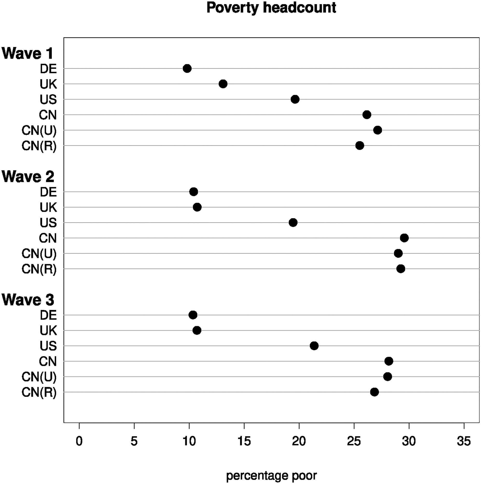
Headcount poverty rate by country and by wave (based on the 60%-of-median-income poverty line).

The headcount rates of Figure 1 refer to the percentage of people who are poor. They do not take into account how far below the poverty line the poor are. To gauge the depth and severity of poverty, I use the well-known Foster–Greer–Thorbecke (FGT) index (Foster et al., 1984). Suppose we observe the income, 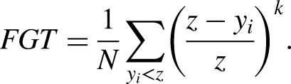$y_{i}$ , of a sample of N individuals, and that z is the poverty line, the FGT index is given by the following expression:

F G T = \frac{1}{N} \sum_{y_{i} < z} {(\frac{z - y_{i}}{z})}^{k} .

The key parameter is k. With

k = 0

, everyone with income below the poverty line contributes the same amount (i.e., 1) to the FGT index. Indeed, this gives the poverty headcount. If

k = 1

, individuals with income further below the poverty line contribute more to the index, as the difference,

z - y_{i}

, is greater for them. This is often referred to as the poverty gap index. With

k = 2

, we get the squared poverty index which gives even greater weight to those with the lowest income. The poverty headcount index, the poverty gap index and the squared poverty index can be taken as measuring the incidence, depth and severity of poverty, respectively (Ravallion, 2016).

Figure 2 reports the poverty gap (left panel) and the squared poverty gap (right panel) of the four countries. They show the same ranking as the poverty headcount index, with Germany and the UK at the low end, China at the high end, and the US in the middle. This ranking holds for all three waves, though the cross-national differences have widened over time. To recap, compared to the three Western countries, not only is relative poverty more common in China, it is also deeper and more severe. Also, while absolute poverty is primarily a rural phenomenon, relative poverty afflicts urban China as much as it does the countryside.

Figure 2.

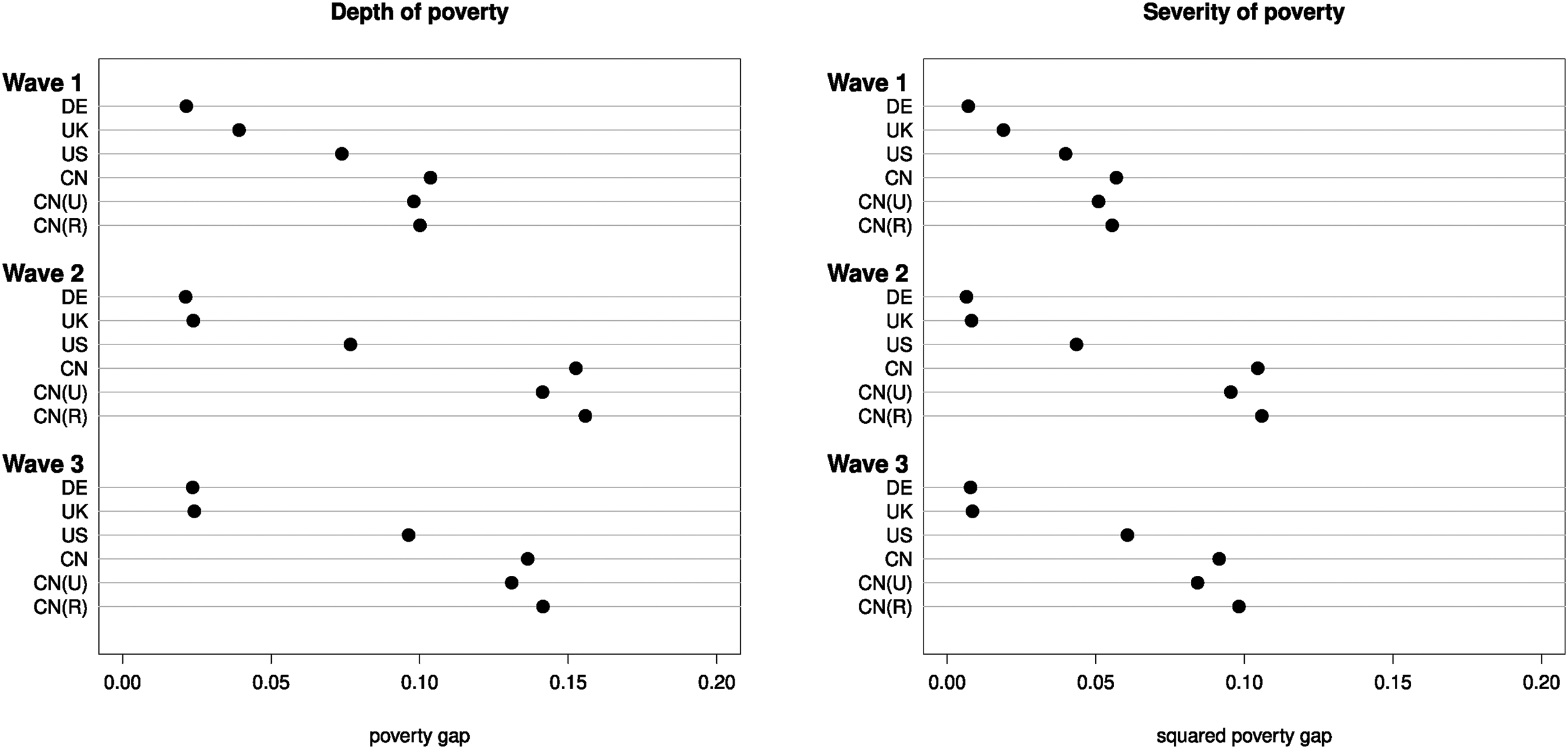
Poverty gap and squared poverty gap by country and by wave (based on the 60%-of-median-income poverty line).

Chronic versus transient poverty

So far, I have analysed the data as though they came from repeated cross-sectional surveys. As a first step to exploit the panel nature of the data, I use a method proposed by Jalan and Ravallion (1998, 2000) to decompose total poverty into its chronic and transient components. They regard someone as chronically poor if her average income over the relevant period is below the poverty line; and transient poverty is defined as “the contribution to expected poverty of the variability over time in the individual welfare indicator” (Jalan and Ravallion, 1998: 341).

Formally, total, chronic, and transient poverty are defined as follows. For a sample of N individuals observed over T periods, let $y_{i t}$ be the normalised income of individual i at time t, and the poverty line is set at 1. Using the squared poverty gap, the poverty experienced by i at t is:

\begin{matrix} p (y_{i t}) & = {\begin{matrix} {(1 - y_{i t})}^{2} & if y_{i t} < 1 \\ 0 & if y_{i t} \geq 1. \end{matrix} \end{matrix}

The total poverty experienced by i over T periods is

P_{i} = T^{- 1} \sum_{t} p (y_{i t})

, and the total poverty for the population is

P = N^{- 1} \sum_{i} P_{i}

Now the average income of individual i is $\bar{y_{i}} = T^{- 1} \sum_{t} y_{i t}$ . The chronic poverty experienced by i is given by:

\begin{matrix} C_{i} & = {\begin{matrix} {(1 - \bar{y_{i}})}^{2} & if \bar{y_{i}} < 1 \\ 0 & if \bar{y_{i}} \geq 1. \end{matrix} \end{matrix}

The level of chronic poverty in the population is

C = N^{- 1} \sum_{i} C_{i}

. The transient poverty experienced by i is the difference between total and chronic poverty, that is,

Q_{i} = P_{i} - C_{i}

. Similarly, the transient poverty for the whole population is defined as

Q = P - C

Figure 3 illustrates the notions of chronic and transient poverty as set out above. Here we observe for 20 periods the income of six hypothetical individuals, labelled A through to F. The mean income (represented by the dotted line) of A, B, and C is above the poverty line (the solid line). So, there is no chronic poverty for them (shown in the top row of Figure 3). The opposite is true of D, E, and F in the bottom row. As their mean income (dotted line) is below the poverty line (solid line), they are chronically poor.

Figure 3.

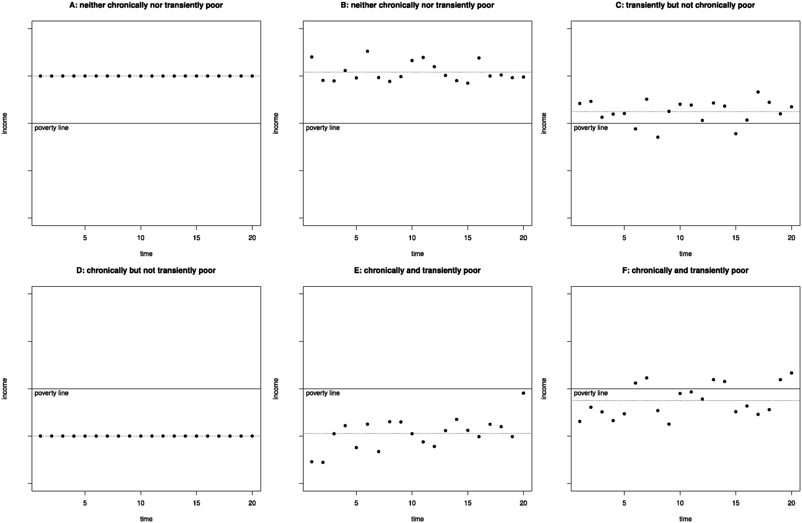
Hypothetical examples of income and poverty status of six individuals over time.

The income of A and D (the top-left and bottom-left panels of Figure 3, respectively) is completely stable over time. A is never poor and so, by definition, never transiently poor. D is always poor. But since D's income never changes, he experiences no transient poverty either. We have already noted that E and F are chronically poor. And since their income varies over time, they experience transient poverty too, even though E's income is always below the poverty line. C is not chronically poor. But her income sometimes drops below the poverty line. So, the only kind of poverty that C experiences is transient in nature. Finally, although B's income varies over time, it is always above the poverty line. Thus, B experiences neither transient nor chronic poverty.

Having explained the meaning of total, chronic, and transient poverty, let us go back to the data. The overall height of the bars in Figure 4 is a measure of the amount of total poverty found over three waves.⁸ Germany is at the low end (0.005), followed by the UK (0.010), the US (0.039) and then China (0.086). Thus, the US has eight times as much total poverty as Germany. But the level of total poverty in China is double that in the US. This is consistent with the pattern in Figures 1 and 2.

Figure 4.

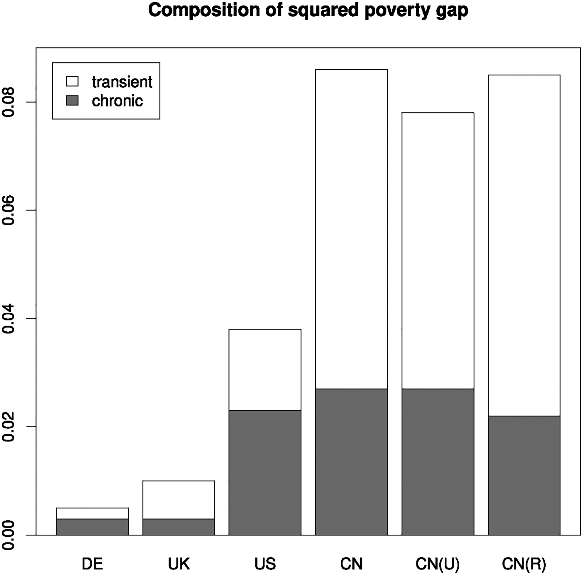
Total, chronic and transient poverty by country (based on the 60%-of-median-income poverty line).

Figure 4 also shows interesting cross-national differences in the composition of total poverty. Transient poverty accounts for less than half of the total poverty of the US (40%) or Germany (44%), but about two-thirds of those of the UK (66%) or China (68%).

Poverty entry and exit

To delve deeper into the cross-national differences in the balance between chronic and transient poverty, let us consider poverty “entry” and “exit”. I have used quotes in the previous sentence because what the biennial panel surveys give us are snapshots of the respondents’ poverty status at the time of the interviews, not what happened in-between. Thus, someone who was found to be poor in both waves 1 and 2 might have stayed poor throughout the two years between the interviews. Or, he might have escaped poverty and then fallen back into it (i.e., a case of recurrent poverty).⁹ It is because of this limitation of the data (and also because the Chinese panel is still very short) that I refrain from carrying out event history analyses of poverty entry and exit (Bane and Ellwood, 1986).

Having stated this caveat, it is useful to consider the following questions. Among people who were not poor at, say, wave 1, what fraction was poor at wave 2? And among those who were poor at wave 1, what fraction were not poor at wave 2? I use poverty entry rate and poverty exit rate as shorthands to refer to these fractions.¹⁰

The left panel of Figure 5 shows that, between waves 1 and 2, the poverty entry rates are 4% for Germany, 6% for the UK, 8% for the US, and remarkably, 25% for China. The right panel of Figure 5 reports the poverty exit rates, which are 41% for Germany, 57% for the UK, 36% for the US and 51% for China. Very similar poverty entry and exit rates are observed if we were to compare the poverty status of individuals between waves 1 and 3 or between waves 2 or 3.

Figure 5.

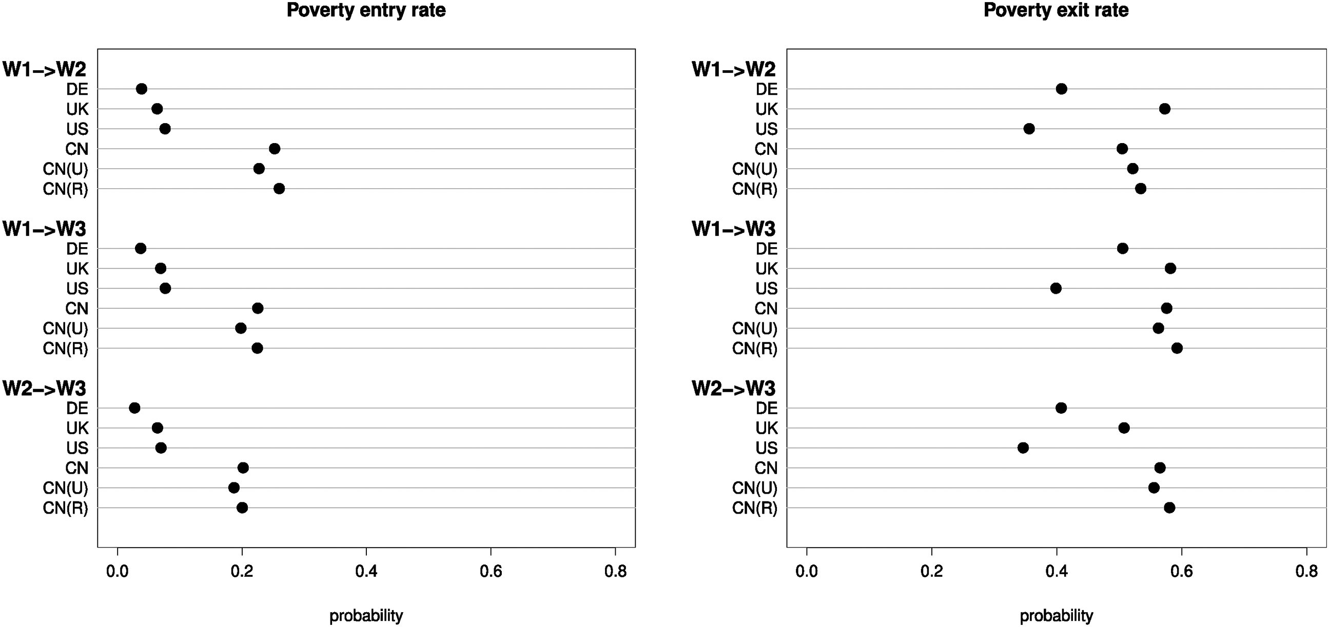
Poverty entry and exit probabilities (based on the 60%-of-median-income poverty line).

Taken together, the entry and exit rates help elucidate the results of Figure 4. For example, China has, by some distance, the highest poverty entry rate and either the highest or the second highest poverty exit rate. This means that, by international standards, the typical Chinese face quite high risks of becoming poor, but they tend not to stay poor for very long. This is consistent with the observation that total poverty in China is at a very high level, and much of it is transient in nature. In sharp contrast to China, Germany has the lowest poverty entry rate and the second lowest poverty exit rate. This is in line with what is shown in Figure 4 where Germany has the lowest level of total poverty, of which just over half is chronic.

Figure 4 also shows that the level of total poverty in the UK is relatively low (when compared to China or the US) and two-thirds of it is transient. This makes sense given the pattern in Figure 5 where the UK's poverty entry rate is closer to Germany's, and its poverty exit rate is comparable to China’s. Finally, the poverty entry rate of the US is slightly higher than those of the UK and Germany, and it has the lowest poverty exit rate of the four countries. Again, this matches with the pattern of Figure 4 where total poverty in the US is high, and three-fifths of which is chronic.

The entry and exit rates of Figure 5 are also relevant to assessing previous cross-national research on poverty dynamics. Recall the observation of Duncan et al. (1993) that countries with higher poverty level tend to have lower poverty exit rates (cell 1 of Table 1) and higher poverty entry rates (cell 2 of Table 1). They also propose a simple mechanism that explains these associations. Specifically, the more poverty there is, the greater the likely distance between the typical poor person and the poverty line (cell 3 of Table 1), and this would explain the lower escape rate. Conversely, where there is less poverty, the typical non-poor person would be further above the poverty line (cell 4 of Table 1), which is why she is less likely to fall into poverty.

The left panel of Figure 5 shows that Germany has the lowest poverty entry rate, followed by the UK, the US and China. As the poverty levels of the four countries follow the same ranking (see Figures 1 and 2), this result is consistent with Duncan et al. (1993).

As regards escaping poverty, the right panel of Figure 5 shows that, between waves 1 and 2, the US has the lowest poverty exit rates, followed by Germany, China and the UK.¹¹ The pattern for the three Western countries is arguably consistent with Duncan et al. (1993). Compared to the US, there is less relative poverty in Germany or the UK, and it is also easier to escape poverty in the two European countries.¹² But when China is considered, the picture looks very different. Although relative poverty is at a very high level in China, poverty exit rates in China are the highest or the second highest of the four countries.

Turning to the proposed mechanism that links relative poverty levels to the poverty entry and exit rates, the left panel of Figure 6 reports the median income of the non-poor of each of the four countries, expressed as a percentage of that country's poverty line. In wave 1, they are 192% in Germany, 200% in the UK, 226% in the US and 219% in China. Thus, the non-poor in China or the US are further above the poverty line than their counterparts in Germany or the UK. But, as has been seen, Americans and, especially, Chinese are at greater risks of falling into poverty than are Germans or British. This is not consistent with the suggestion by Duncan et al. (1993) that “the greater …the likely distance between the typical nonpoor family and the poverty threshold and the less likely that family is to make the transition”.

Figure 6.

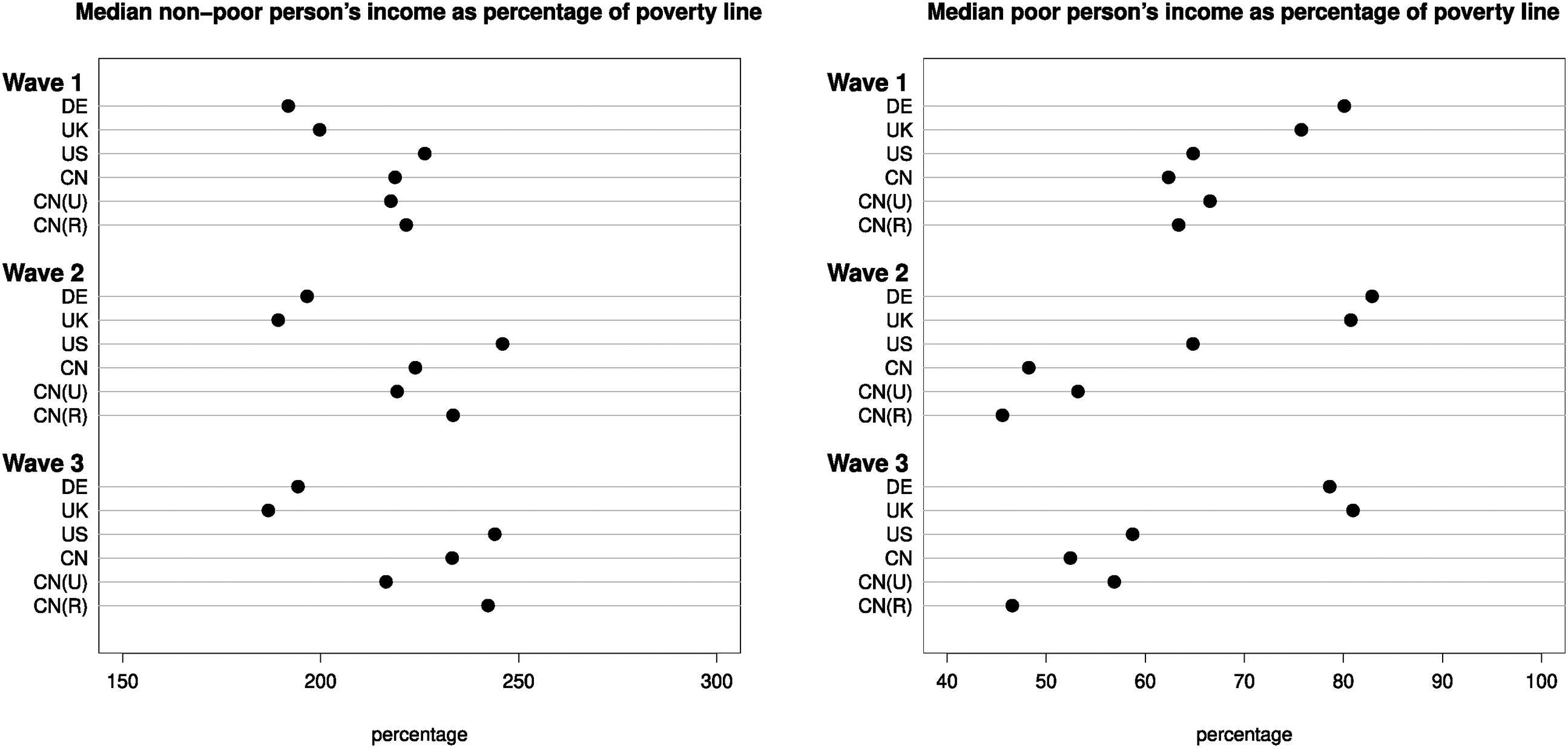
Median non-poor person's (left panel) and median poor person's (right panel) income as a percentage of the poverty line (based on the 60%-of-median-income poverty line).

The right panel of Figure 6 reports the median income of the poor of the four countries, again expressed as a percentage of each country's poverty line. In wave 1, they are 80% for Germany, 76% for the UK, 65% for the US, and 62% for China. Thus, consistent with Duncan et al. (1993), the typical poor person of the two countries with less poverty (i.e., Germany and the UK) are indeed closer to the poverty line than their counterparts in the countries with more poverty (i.e., China and the US). But, contra Duncan et al. (1993), proximity to poverty line does not always imply higher escape rate, for example, compare Germany with China. Overall, it seems clear that poverty entry (exit) rate is not simply a function of how far the non-poor (the poor) are from the poverty threshold.

Occasional and recurrent poverty

A third way to exploit the panel nature of the data is to count how many times someone is poor over three waves. Figure 7 reports the cumulative experience of poverty: 87% of Germans, 78% of British, and 71% of Americans were never poor over three waves. The corresponding figure for China was only 46%. Comparing Figure 7 with Figure 1, it is clear that in all four countries poverty is a more common experience when a longitudinal perspective is taken. This is consistent with both expectation and past research (Layte and Whelan, 2003). But the stark contrast shown in Figure 7 is that while only a minority of individuals in the West were touched by poverty over three waves, being poor was actually the experience of a small majority of Chinese.

Figure 7.

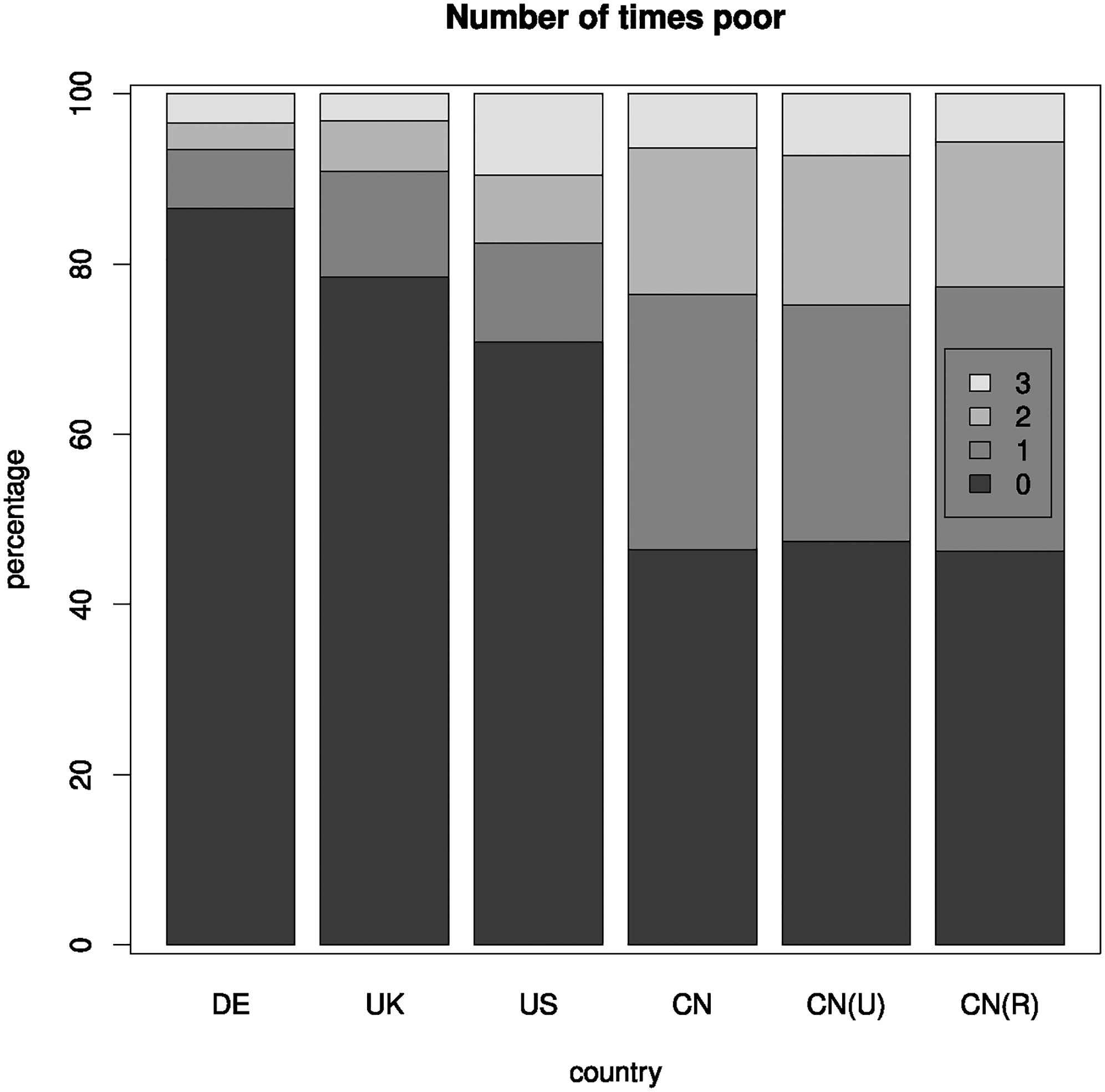
Cumulative experience of poverty over three waves by country (based on the 60%-of-median-income poverty line).

For brevity, I refer to being poor once over three waves as occasional poverty and being poor twice or thrice as recurrent poverty. Using this shorthand, Figure 7 shows that 7% of Germans, 12% of British, 12% of Americans, and 30% of Chinese were occasionally poor; and 6% of Germans, 9% of British, 18% of Americans, and 24% of Chinese were recurrently poor. Thus, the experience of both occasional poverty and recurrent poverty are, by quite a large margin, more common in China.

Determinants of occasional or recurrent poverty

To find out the determinants of occasional or recurrent poverty, I fit a multinomial logit model to the data, with the threefold distinction of never poor, occasionally poor, and recurrently poor as the dependent variables. As regards the independent variables, they include the respondents’ age (at wave 1), sex, family structure (at wave 1, four categories) and urban (vs rural) residence, and three key predictors of income: educational attainment (four categories); employment status; and the additional-earner-to-household-size ratio.¹³ Finally, for China only, I include hukou as a predictor of poverty. All but two of these variables, as constructed, are time-constant in nature. The exceptions are employment status and the additional-earner-to-household-size ratio. For these two variables, I take the mean of their values over three waves.¹⁴ Descriptive statistics of the variables can be found in Table A1 in the Online Appendix.

The results are reported in Table 3. Overall, there is a good deal of cross-national similarity in the determinants of poverty. For example, age (within the age range of 31–55) and gender tend not to predict poverty status. The main exception is the US where men are less likely to be poor.

Table 3.

Multinomial logit model predicting occasionally poor and recurrently poor versus never poor (based on the 60%-of-median-income poverty line).

	Germany		United Kingdom		United States		China		China (urban)		China (rural)
Poor once over three waves versus never poor
	coeff	s.e.	coeff	s.e.	coeff	s.e.	coeff	s.e.	coeff	s.e.	coeff	s.e.
Age	0.022	0.014	0.001	0.005	-0.008	0.010	-0.004	0.004	-0.011	0.007	0.013*	0.006
Male	0.050	0.205	-0.097	0.071	-0.279*	0.141	0.032	0.063	0.010	0.096	0.021	0.080
Junior high ^a	-0.248	0.301	-0.263**	0.095	-0.652	0.407	-0.355**	0.068	-0.371**	0.114	-0.564**	0.087
Senior high	0.411	0.443	-0.504**	0.134	-1.294**	0.323	-0.581**	0.097	-0.699**	0.136	-0.316*	0.139
Post-secondary	-0.459	0.345	-0.803**	0.100	-2.047**	0.319	-1.764**	0.201	-1.745**	0.205	-1.924**	0.523
Mean number employed/household	-3.134**	0.496	-3.083**	0.236	-3.691**	0.481	-1.537**	0.223	-1.795**	0.333	-1.360**	0.294
Mean employed	-2.166**	0.244	-1.144**	0.088	-1.851**	0.225	-0.364**	0.112	-0.411**	0.149	0.223	0.167
Single parent ^b	0.997**	0.360	0.523**	0.133	0.571	0.310	0.703*	0.336	0.714	0.476	0.788	0.459
Couple with children	-0.119	0.272	-0.160	0.100	-0.464*	0.219	-0.180	0.140	-0.040	0.199	-0.342	0.191
Others	0.316	0.310	-0.150	0.131	0.228	0.250	-0.087	0.141	0.074	0.202	-0.159	0.191
Urban	-0.811**	0.198	-0.083	0.083	-0.278	0.174	-0.171*	0.068
Hukou (urban)							-0.658**	0.091	-0.522**	0.105	-0.630**	0.204
Constant	-0.565	0.794	0.194	0.276	3.086**	0.686	1.237**	0.296	1.545**	0.427	-0.286	0.375
Poor once over three waves versus never poor
	coeff	s.e.	coeff	s.e.	coeff	s.e.	coeff	s.e.	coeff	s.e.	coeff	s.e.
Age	0.024	0.016	0.009	0.006	-0.010	0.009	-0.006	0.005	-0.005	0.008	-0.004	0.007
Male	-0.118	0.256	-0.028	0.096	-0.412**	0.156	0.108	0.070	-0.008	0.108	0.170	0.093
Junior high ^a	-0.127	0.298	-0.324**	0.115	-1.049**	0.368	-0.496**	0.076	-0.513**	0.121	-0.516**	0.101
Senior high	-1.183*	0.471	-0.522**	0.165	-2.372**	0.323	-0.787**	0.118	-0.855**	0.156	-0.642**	0.187
Post-secondary	-1.554**	0.356	-1.044**	0.126	-3.481**	0.318	-2.881**	0.382	-2.801**	0.361	-1.903**	0.703
Mean number employed/household	-6.827**	0.821	-4.583**	0.335	-8.891**	0.615	-3.264**	0.257	-3.333**	0.367	-3.189**	0.359
Mean employed	-3.822**	0.317	-2.075**	0.107	-3.174**	0.239	-0.324**	0.120	-0.297	0.163	-0.051	0.180
Single parent ^b	2.115**	0.456	0.779**	0.165	1.234**	0.328	0.473	0.310	1.243**	0.449	0.401	0.432
Couples with children	-0.061	0.384	-0.464**	0.150	0.122	0.271	-0.763**	0.146	0.003	0.220	-1.134**	0.198
Others	1.473**	0.374	0.120	0.157	0.748*	0.289	-0.617**	0.147	-0.169	0.225	-0.960**	0.197
Urban	-0.363	0.248	-0.016	0.106	-0.630**	0.173	-0.491**	0.078
Hukou (urban)							-1.021**	0.114	-1.088**	0.122	-1.336**	0.332
Constant	-0.082	0.837	0.224	0.362	6.007**	0.693	2.270**	0.319	1.885**	0.484	1.629**	0.416
n	5122		10,611		3659		11,371		4652		6212
R ²	0.273		0.175		0.279		0.076		0.088		0.034

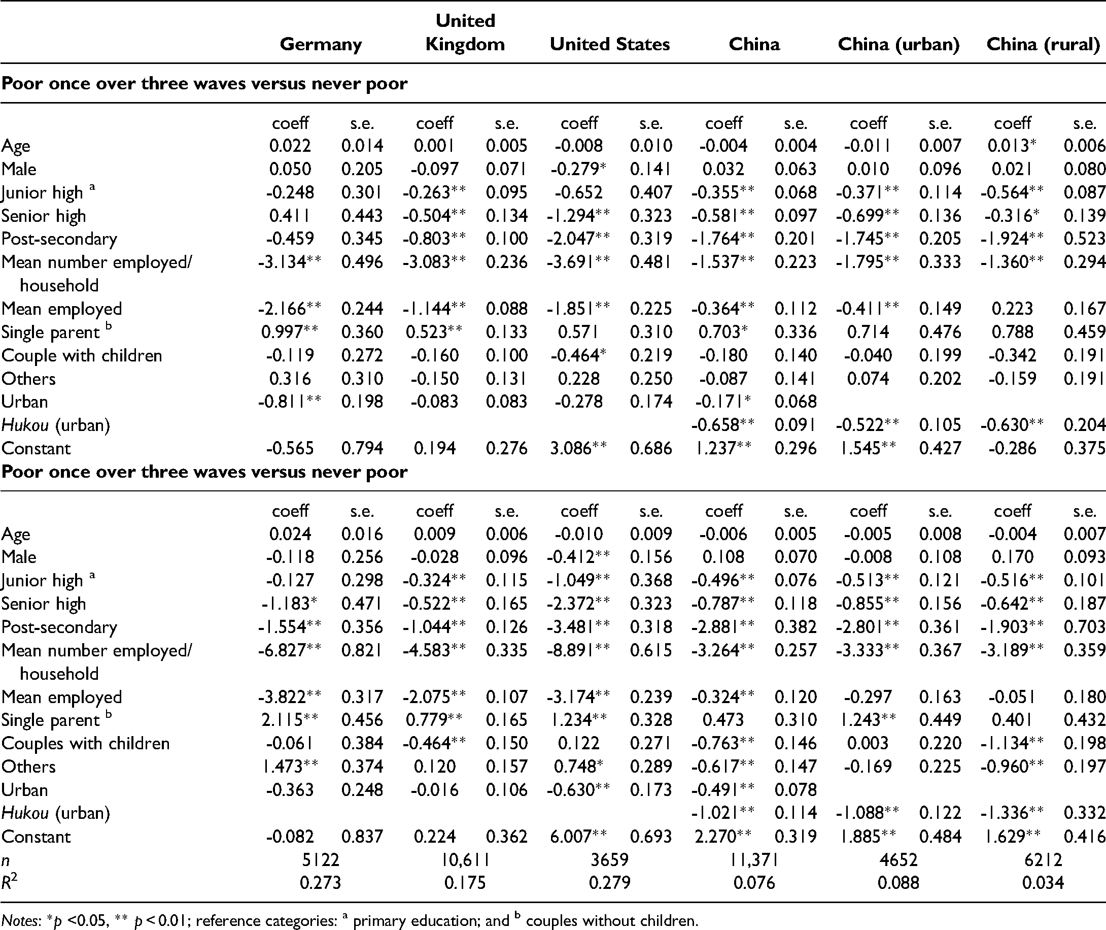
Notes: *p <0.05, ** p < 0.01; reference categories: ^a primary education; and ^b couples without children.

People with more education are everywhere less likely to be poor, except for the contrast between occasionally poor and never poor in Germany. Similarly, in all countries, having more earners in the household and being employed protect against poverty. But it is notable that the magnitude of these employment-related parameters is considerably smaller in China. Indeed, when urban and rural China are examined separately, being employed only protects against occasional poverty in urban China.

As regards family structure, compared to the reference category of couples without children, single-parents are more likely to be poor; while couples with children are less likely to be occasionally poor in the US, and they are less likely to be recurrently poor in the UK and China.

In China, Germany and the US, but not in the UK, people living in rural areas are more likely to be poor: occasionally in Germany; recurrently in the US; and both occasionally and recurrently in China. As expected, Chinese with urban hukou are less likely to be poor.

But the most remarkable result of Table 3 is that the pseudo- $R^{2}$ of the multinomial logit model is much smaller for China (8%) than for the other three countries (18% to 28%). Thus, while many key determinants of poverty work in similar ways in the four countries, being poor is a much more unpredictable experience for Chinese.

Given the large regional difference in living standards in China, I have, in a further model (not shown), controlled for regions, that is, the Bundesländer in Germany, the government regions in the UK, the states in the US, and the provinces in China.¹⁵ It turns out that adding region to the model increases the pseudo- $R^{2}$ slightly: from less than 1% in the UK to 3% in China. Thus, even with regional differences accounted for, there is still a large gap in the variance explained between China and the three Western countries.

Summary and discussion

China has made some truly significant progress in tackling absolute poverty. But relative poverty is a different story altogether. Compared to Germany, the UK, and the US, not only is relative poverty more common in China, it is also deeper and more severe. Furthermore, while absolute poverty in China is “predominantly a rural phenomenon”, relative poverty afflicts Chinese cities as much as it does the countryside.

By international standards, a very large share of China's relative poverty is transient in nature. (Transient poverty is also important in the UK. A point that I will return to later.) Direct measures of poverty entry and exit rates also suggest greater instability of people's economic fortune in China. Compared to their Western counterparts, the average Chinese faces significantly higher risks of falling into relative poverty. But the relatively poor in China are also more likely to escape poverty than the poor in Germany or the US.

The combination of high poverty entry rate and high poverty exit rate means that there are more occasional poverty and more recurrent poverty in China than in the West. Indeed, while a minority of people in Germany, the UK and the US were touched by relative poverty over three waves (four years), being poor was actually the experience of a small majority of Chinese.

Relative poverty in China is distinctive in many ways. But we should not regard China as sui generis, as the covariates predicting poverty status are very similar across the four countries. For example, higher educational qualifications, employment, and having more earners in the household all protect against poverty in the four countries. But collectively these covariates are much less predictive of poverty status in China than in Germany, the UK and the US.

The findings of this paper also speak to our understanding of poverty dynamics in general. Duncan et al. (1993) posit that countries with more poverty tend to have higher poverty entry rates, and that is because the non-poor in those countries tend to be closer to the poverty line. We do observe higher poverty entry rates in countries with more poverty. But the non-poor of those countries (e.g., China and the US) are actually further away from the poverty line than their counterparts in countries with less poverty (e.g., Germany and the UK).

Furthermore, Duncan et al. (1993) argue that poverty exit rates would be lower in countries with more poverty, as the typical poor person in those countries would be further below the poverty line. Once again, this is only partly true. The median poor person in China or the US are indeed further away from the poverty lines than the median poor person in Germany or the UK. But poverty exit rates are much higher in China or the UK than in Germany or the US.

Some revisions to Duncan et al. (1993) are therefore necessary. Mechanically speaking, it is a large income change that pushes people into poverty or plucks them out of it. What counts as a large income change depends partly on how far someone is from the poverty threshold. This is why the claims of Duncan et al. (1993) are eminently reasonable. But our findings show that this is not the whole story. Other social forces operating in the labour market, in households and in the broader policy environment also make large income changes more likely to occur in some countries than in others.

For example, using the same data sets, Chan et al. (2019) show that not only is permanent income more unequally distributed in China than in the West, but there is greater instability in transitory income in China too. They decompose the total variance of log-income in the panel data into its between and within components, and report that “in Germany, the UK, and the US the lion's share of income inequality is found between individuals rather than within individuals. But the opposite is true for China, suggesting that the average Chinese face a much higher degree of income instability and uncertainty” (Chan et al., 2019: 443). Moreover, while there is regression to the mean in income in all four countries, “the magnitude of income change is always larger in China than in the three Western countries” (Chan et al., 2019: 439). They then argue that broader changes in the labour market and employment practices in China have created a large pool of casually employed workers which, in turn, explains the heightened income instability in China (Gallagher, 2005; Kuruvilla et al., 2011).

Finally, the implications of the findings of this paper go beyond China. In comparative research on welfare capitalism, the UK and the US are often grouped together as exemplars of the liberal regime. Similarly, Atkinson (2015: 20) notes that, so far as inequality is concerned, “the situation in the UK is a pale imitation of what is happening in the US, and that the UK chart can be obtained by simply replacing ‘S’ by ‘K’ in the heading. There is some truth in this. But the poverty dynamics of the two countries is actually quite different. In particular, rates of poverty exit are much higher in the UK than in the US (see also Office for National Statistics, 2015; Vaalavuo, 2015; Valletta, 2006). This means that there is much less chronic poverty in the UK. This is a particularly intriguing outcome as many of the anti-poverty policies brought in by the New Labour government (1997–2010), for example, tax credits, were “strongly influenced by evidence from US welfare-to-work experiments and, again, had many elements common with them” (Waldfogel, 2010: 5). Further work on how the social structure and/or anti-poverty programmes of the UK and US had led to such different poverty dynamics would be very illuminating.

Supplemental Material

sj-pdf-1-chs-10.1177_2057150X211068543 - Supplemental material for The dynamics of relative poverty in China in a comparative perspective

Supplemental material, sj-pdf-1-chs-10.1177_2057150X211068543 for The dynamics of relative poverty in China in a comparative perspective by Tak Wing Chan in Chinese Journal of Sociology

Footnotes

Declaration of Conflicting Interests

The author declared no potential conflicts of interest with respect to the research, authorship, and/or publication of this article.

Funding

The authors disclosed receipt of the following financial support for the research, authorship, and/or publication of this article: This work was supported by the Economic and Social Research Council (Grant number: ES/L015927/1).

ORCID iD

Tak Wing Chan

Supplemental material

Supplemental material for this article is available online.

Notes

References

Appleton

Song

Xia

(2010) Growing out of poverty: Trends and patterns of urban poverty in China. World Development 38(5): 665–678.

Appleton

Song

Xia

(2014) Understanding urban wage inequality in China 1988–2008: Evidence from quantile analysis. World Development 62: 1–13.

Atkinson

(2015) Inequality: What can be Done? Cambridge, MA: Harvard University Press.

Atkinson

(2019) Measuring Poverty Around the World. Princeton, NJ: Princeton University Press.

Bane

Ellwood

(1986) Slipping into and out of poverty: The dynamics of spells. Journal of Human Resources 21(1): 1–23.

Chan

Zhang

(1999) The Hukou system and rural–urban migration in China: Processes and changes. China Quarterly 160: 818–855.

Chan

Ermisch

Gruijters

(2019) The dynamics of income inequality: The case of China in a comparative perspective. European Sociological Review 35(3): 431–446.

Chen

Ravallion

Wang

(2006) Di Bao: A guaranteed minimum income in China’s cities. Policy Research Working Paper WPS3805, The World Bank. Available at: https://documents1.worldbank.org/curated/en/399721468019146622/pdf/wps3805.pdf (accessed 18 May 2018).

Park

Wang

(2005) Migration and rural poverty in China. Journal of Comparative Economics 33(4): 688–709.

10.

Duncan

Gustafsson

Hauser

, et al. (1993) Poverty dynamics in eight countries. Journal of Population Economics 6(3): 215–234.

11.

Foster

Greer

Thorbecke

(1984) A class of decomposable poverty measures. Econometrica 52(3): 761–766.

12.

Fouarge

Layte

(2005) Welfare regimes and poverty dynamics: The duration and recurrence of poverty spells in Europe. Jounal of Social Policy 34(3): 407–426.

13.

Gallagher

(2005) Contagious Capitalism: Globalization and the Politics of Labor in China. Princeton, NJ: Princeton University Press.

14.

Gottschalk

Moffitt

(2009) The rising instability of U.S. earnings. Journal of Economic Perspectives 23(4): 3–24.

15.

Gustafsson

Deng

(2011) Di Bao receipt and its importance for combating poverty in urban China. Poverty and Public Policy 3(1): 1–32.

16.

Gustafsson

Sai

(2009) Temporary and persistent poverty among ethnic minorities and the majority in rural China. Review of Income and Wealth 55(Suppl 1): 588–606.

17.

Gustafsson

Zhong

(2000) How and why has poverty in China changed? A study based on microdata for 1988 and 1995. China Quarterly 164: 983–1006.

18.

Jalan

Ravallion

(1998) Transient poverty in postreform rural China. Journal of Comparative Economics 26(2): 338–357.

19.

Jalan

Ravallion

(2000) Is transient poverty different? Evidence from rural China. Journal of Development Studies 36(6): 82–99.

20.

Jäntti

Danziger

(2000) Income poverty in advanced countries. In: Atkinson

Bourguignon

(eds) Handbook of Income Distribution, Volume 1, Chapter 6. Amsterdam: Elsevier, 309–378.

21.

Jenkins

(2011) Changing Fortunes: Income Mobility and Poverty Dynamics in Britain. Oxford: Oxford University Press.

22.

Kuruvilla

Lee

Gallagher

(2011) From Iron Rice Bowl to Informalization: Markets, Workers, and the State in a Changing China. Ithaca, NY: ILR Press.

23.

Layte

Whelan

(2003) Moving in and out of poverty. European Societies 5(2): 167–191.

24.

Sicular

(2014) The distribution of household income in China: Inequality, poverty and policies. China Quarterly 217: 1–41.

25.

Luo

Sicular

(2013) Overview: Income and poverty in China, 2002–2007. In: Li

Sato

Sicular

(eds) Rising Inequality in China: Challenges to a Harmonious Society, Chapter 2. Cambridge: Cambridge University Press, 44–84.

26.

Liang

(2014) Changing patterns of the floating population in China, 2000–2010. Population and Development Review 40(4): 695–716.

27.

Meng

Gregory

(2007) Urban poverty in China and its contributing factors, 1986–2000. Review of Income and Wealth 53(1): 167–189.

28.

Office for National Statistics (2015) Persistent poverty in the UK and EU: 2008–2013. Technical report, Office for National Statistics, London. Available at: https://www.ons.gov.uk/peoplepopulationandcommunity/personalandhouseholdfinances/incomeandwealth/articles/persistentpovertyintheukandeu/2015-05-20 (accessed 7 December 2020).

29.

(1989) State and Peasant in Contemporary China: The Political Economy of Village Government. Berkeley, CA: University of California Press.

30.

Park

Wang

(2010) Migration and urban poverty and inequality in China. China Economic Journal 3(1): 49–67.

31.

Ravallion

(2014) An emerging new form of social protection in twenty-first-century China. In: Fan

Kanbur

Wei

S-J

Zhang

(eds) The Oxford Companion to the Economics of China. Oxford: Oxford University Press, 441–444.

32.

Ravallion

(2016) The Economics of Poverty: History, Measurement and Policy. Oxford: Oxford University Press.

33.

Ravallion

Chen

(2007) China’s (uneven) progress against poverty. Journal of Development Economics 82(1): 1–42.

34.

Shorrocks

Davies

Lluberas

(2019) Global wealth report 2019. Technical report, Credit Suisse Research Institute. Available at: http://docs.dpaq.de/17706-global-wealth-report-2021-en.pdf (accessed 21 October 2019).

35.

Smeeding

Rainwater

Burtless

(2002) U.S. Poverty in a cross-national context. In: Danziger

Haveman

(eds) Understanding Poverty, Chapter 5. Cambridge, MA: Harvard University Press, 162–189.

36.

Vaalavuo

(2015) Poverty dynamics in Europe: from what to why. Working paper 03/2015, European Commission, Luxembourg.

37.

Valletta

(2006) The ins and outs of poverty in advanced economies: Government policy and poverty dynamics in Canada, Germany, Great Britain, and the United States. Review of Income and Wealth 52(2): 261–284.

38.

Waldfogel

(2010) Britain’s War on Poverty. New York: Russell Sage Foundation.

39.

Whyte

(2005) Rethinking equality and inequality in the PRC. In: 50th Anniversary conference for the Fairbank Center for East Asian Research, Harvard University. Available at: https://datascience.iq.harvard.edu/files/wcfia/files/1068_mkw_rethinkingequality.pdf (accessed 21 November 2016).

40.

World Bank (2009) From Poor Areas to Poor People: China’s Evolving Poverty Reduction Agenda—an Assessment of Poverty and Inequality. Washington, DC: World Bank.

41.

Xie

(2013) Introduction. In: Xie

Zhang

, et al. (eds) China Family Panel Studies 2013, Chapter 1. Beijing: Peking University Press, 1–26.

42.

Xie

Zhou

(2014) Income inequality in today’s China. Proceedings of the National Academy of Scineces of the United States of America 111(19): 6928–6933.

43.

Xie

Zhang

, et al. (2015) Short-term trends in China’s income inequality and poverty: Evidence from a longitudinal household survey. China Economic Journal 8(3): 235–251.

44.

Zhang

Zhou

, et al. (2014) Are poverty rates underestimated in China? New evidence from four recent surveys. China Economic Journal 31: 410–425.

Supplementary Material

Please find the following supplemental material available below.

For Open Access articles published under a Creative Commons License, all supplemental material carries the same license as the article it is associated with.

For non-Open Access articles published, all supplemental material carries a non-exclusive license, and permission requests for re-use of supplemental material or any part of supplemental material shall be sent directly to the copyright owner as specified in the copyright notice associated with the article.

0.00 MB

0.10 MB