Modeling of a controlled flow cup for improved transitional drinking development in children

Abstract

Introduction

Clinical observations of children with swallowing disorders using a traditional “sippy” or transitional drinking cup identified a need for a novel cup. Children with swallowing disorders are often unable to initiate the forces required to activate the cup and/or maintain suction pressure. Furthermore, fast flow rates can result in choking.

Methods

A new cup design tool is proposed using fluid-cup interactions to capture the changing geometry of the fluid during drinking. A Petri net formulation is integrated with standard fluid flow principles. A new parametric cup simulation provides visualization and direct implementation for microcontroller prototypes. A vent-based controller is developed and modeled for a novel transitional drinking cup design. A simulated pouring study is performed for water and a baseline liquid volume of 200 ml in the cup. The study varies rotation rates, initial volume, system control and desired flow rates.

Results

Volumetric flow rate curves over time are generated and compared in relation to a target flow rate. The simulation results show expected behavior for variations in cup parameters.

Conclusion

The new simulation model facilitates future dysphagia research through rapid prototyping by tuning cup geometry, liquid parameters and control signals to meet the varying needs of the users.

Introduction

Clinical observation of both typically developing children and children with swallowing disorders while using traditional “sippy” or transitional drinking cups identified a need for a novel delivery system. In order to develop an innovative solution to this need, a holistic approach was employed including generation of a model and subsequent computer simulation, and a critical examination of the components of the system design. Through our early work we found that there are no existing mathematical models or simulations which integrate fluid flow models, discrete changes in fluid geometry, and real time monitoring and control of the system states.

The current state of “sippy” cup or transition cup design used in Western societies are variations of an original patent ¹ which introduced a lid with a wide thin raised extension, or embedded spout. Since that time, hundreds of derivations of this original model have been on the commercial market most which now have a “no flow” or “no spill” feature added. These commercially available “no flow” cups have a wide range of suction pressures required to break a no-spill vacuum and variable amounts of continuous suction pressure required to maintain fluid flow. ² Both issues are problematic for some typically developing children as well as children with swallowing difficulties. Furthermore, these transition cups with a nipple like extension have become “nothing more than a baby bottle in disguise”. ³ As a result the current sippy cup can cause a myriad of issues during normal child maturation, such as improper speech development, development of abnormal dental occlusion patterns, otitis media, iron deficiencies and/or dental caries.^4–6 For children with swallowing disorders, the “sippy” cup is often an obsolete option because the child is unable to initiate the initial forces required to activate the cup and/or maintain suction pressure throughout. Further, modifications of the cup to eliminate suction pressure (i.e. the stopper is removed) results in a rapid change to a fast flow rate of the fluid, resulting in choking. In addition, children with swallowing disorders may be transitioning from bottle drinking or from alternative feeding tubes directly to open-cup drinking, ² thus necessitating different needs within cup design parameters.

In order to solve the problem with a transition cup having a “nipple-like” extension, in 2011, another training cup emerged on the market that uses a regular drinking cup with a baffling system inserted into the cup. ⁷ Although this new invention solved the issue of a nipple-like extension and slows the flow compared to an open-cup, the design did not allow for adjustments to meet individual user needs. Therefore, a need exists for a controlled flow drinking cup to improve the drinking behavior of children both with and without swallowing disorders.

The modeling and development of a new controlled flow cup requires an understanding of the necessary flow rates for the intended users. An examination of existing literature has failed to identify a known range of volumetric flow that is achieved by typically developing children or children with swallowing difficulties. However, preliminary data with typically developing preschoolers (ages, 36-58 months) were recruited for a study that examined volume and temporal parameters during swallowing of puree and liquid consistencies. All subjects displayed discrete swallows under 3.0 ml volumes. ⁸ This discrete swallow volume data can be utilized as a lower bound for the volumetric flow rates that provide target flow rates for the development of a controlled flow cup.

Drinking fluid from a cup is a complex interaction between the physical constraints of the cup, the properties of the fluid, and the behavior of the user. For simplification, the effects of the cup user (sucking or regulating flow) are disregarded for developing a new cup model. The physical drinking mechanism assumed for this work is a closed container with a drinking aperture and a vent hole instead of alternate mechanisms such as an open-cup or a lid with a straw. Furthermore, a thin fluid is assumed.

The models for fluid pouring from a static container (tank) as a result of gravity is well established and are often characterized as liquid-level systems. ⁹ Appropriate models for fluid flow from a cylinder (cup) rotating around an axis perpendicular to the cylinder’s axis have not been found in existing literature. However, two models that assume a rectangular open container were developed to study the efficiency of pouring viscous fluids ¹⁰ and visually controlled pouring over an open container lip. ¹¹ In both of these models, the cup shape and lack of lid invalidate the geometrical assumptions of the proposed “sippy” cup model. Furthermore, the intent of the proposed model is to codify the system states within a microcontroller. The limited microcontroller memory precludes the utilization of modelling and analysis with computational fluid dynamic models (CFD).

Therefore, a need exists for a model of cup pouring behavior that can be incorporated into the controls of a regulated flow drinking cup targeted at children transitioning from bottle to open-cup drinking. This paper presents a model framework for a fluid flow simulation that accounts for cup geometry. Subsequently, the closed valve controller model is developed. Results are presented and analyzed for a cup pouring water with and without controlled flow. Conclusions from these simulated studies and the future integration of the model into a physical prototype cup are discussed.

Model for cylindrical cup fluid flow

In order to simplify the model, the cup configuration is assumed to be a cylindrical vessel with a closed lid that has a drinking aperture and a vent hole. The cup design has integrated sensors to provide the drinking angle or cup rotation, α, and weight of the liquid, w. The model assumes that the cup is not completely filled with liquid and that the remainder of the cup volume is air. This mimics typical cup filling behavior where the liquid does not reach the brim of the cup. The liquid level is modelled by defining four liquid variables in the plane that passes through the drinking aperture and the vent hole and is perpendicular to the base of the cup. It is assumed that rotation about the cylindrical axis is minimal since the expected behavior during use of the cup would have the drinking aperture approaching the mouth and the cup tilting toward the mouth. The drinking angle denotes the rotation of the cup within this plane from vertical. The liquid variables denote the position of the leading edge and the trailing edge of the liquid in the plane where the leading edge is defined by the point closest to the drinking aperture. The height along the leading edge is denoted by h_L, the distance along the top at the leading edge is denoted by x_L, the height of the trailing edge is denoted by h_T, and the distance along the bottom at the trailing edge is denoted x_T (Figure 1). The initial height of the liquid, h₀, is defined when the cup rotation angle, α, is zero.

Figure 1.

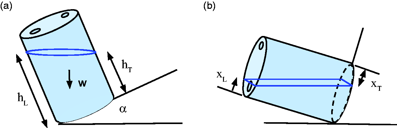
Definition of variables for liquid tilted in a cylindrical cup. Height variables (a) and distances along the top/bottom (b) for the leading and trailing edge of the liquid in a tilted cup.

Determination of leading edge height of liquid

In order to determine when liquid is present at the drinking aperture, the vertical height of the liquid, h_Z, in the cross sectional plane is calculated in reference to the vertical height of the drinking aperture, d (Figure 2). Cup geometry is assumed to be known and input into the model. The drinking aperture hole is assumed to be circular.

Figure 2.

Drinking aperture variables (d,d_max,d_min) and liquid height (h_Z) in the model plane.

The vertical height of the drinking aperture is determined utilizing the radial distance from the leading edge of the top of the cup to the center of the drink aperture, x_D, the drink aperture diameter, φ_D, and the cup height, h_C. The vertical height of the center of the drinking aperture, d, as well as the minimum, d_min, and maximum, d_max, can be calculated using the cup variables and the drinking angle.

$$d=h_C\mathrm{ }\cos \mathrm{ }\left(\alpha \right)+x_D\mathrm{\hspace{0.17em}}\text{sin}\mathrm{\hspace{0.17em}}\left(\alpha \right)$$

(1)

$$d_{\min }=d-\frac{\varphi d}{2}\mathrm{ }\text{sin}\left(\alpha \right)$$

(2)

$$d_{\mathit{max}}=d+\frac{\varphi d}{2}\mathrm{ }\text{sin}\left(\alpha \right)$$

(3)

The key threshold for liquid leaving the cup is when the vertical level of the liquid meets the minimum edge of the drinking aperture which can be represented by the following condition.

$$h_Z\mathrm{ }\ge d_{\min }$$

(4)

The vertical liquid height, h_Z, can be determined based on the liquid variables, h_L and x_L, and the cup rotation, α, as per equation (5).

$$h_Z=\mathrm{ }{h}_L\text{cos}\left(\alpha \right)+x_L\text{sin}\left(\alpha \right)$$

(5)

When the cup initially tilts from 0 degrees, the height of the liquid is completely determined from the h_L term since the x_L term is zero until the liquid comes in contact with the lid. Once the liquid comes in contact with the lid, the x_L term is accounted for in the liquid height calculation. At 90 degrees, the cosine term will go to 0 and the height of the liquid will equal x_L. The liquid shape variables h_L, x_L, h_T, and x_T change as the cup rotates and as liquid leaves the cup. The dynamic cup simulation model updates the liquid variables at each time step during cup rotation. The proposed cup tracks the volume via weight. Therefore, the relationship between the liquid variables and the 3-dimensional geometry of the liquid volume as the cup tilts from a vertical position is important. Each volumetric shape of the liquid can represent a system state.

Using volume formulas for the liquid at each of these geometric system states, the liquid level (the four liquid variables) within the cup can be determined. The transitions between the distinct geometric states are based on discrete events related to the liquid transitioning along the internal surface of the cup. Petri net models are utilized to describe the behavior of discrete event dynamic systems. ¹² It is proposed that a petri net model can be utilized to transition between different sub-models for system prediction in the cup control scheme.

Petri net model of liquid states

As the cup tilts, a discrete event petri net model based on the angle and the liquid interaction with the top and bottom surfaces can be defined by the places listed in Table 1, the transitions listed in Table 2, and four inhibitor arcs based on the physical constraints of cup-liquid interaction. It is assumed that the cup is not completely full so there is some air in the cup and that the cup is not being modelled when completely empty (the end state). Thus, two inhibitor arcs account for the fact that liquid in a vertical cup cannot have partial contact with the bottom or top of the cup. Two inhibitor arcs account for the fact that the liquid in a horizontal cup must have partial contact with the top and bottom. The resulting petri net diagram for the cup states is Figure 3.

Table 1.

System places for Petri Net model of cup.

Place	Description
p1	Cup is vertical. (a = 0)
p2	Cup is tilted between 0 and 90 degrees
p3	Cup is horizontal
p4	Liquid contacts complete bottom.
p5	Liquid contacts part of bottom surface
p6	Liquid does not contact top
p7	Liquid contacts part of top surface

Table 2.

System transitions for Petri Net model of cup.

Transition	Description
t1	Cup tilts from vertical
t2	Cup tilts to horizontal
t3	Cup tilts to vertical
t4	Cup tilts from horizontal
t5	Liquid loses full contact with bottom surface
t6	Liquid fully covers bottom surface
t7	Liquid contacts the top surface
t8	Liquid loses full contact with the top surface

Figure 3.

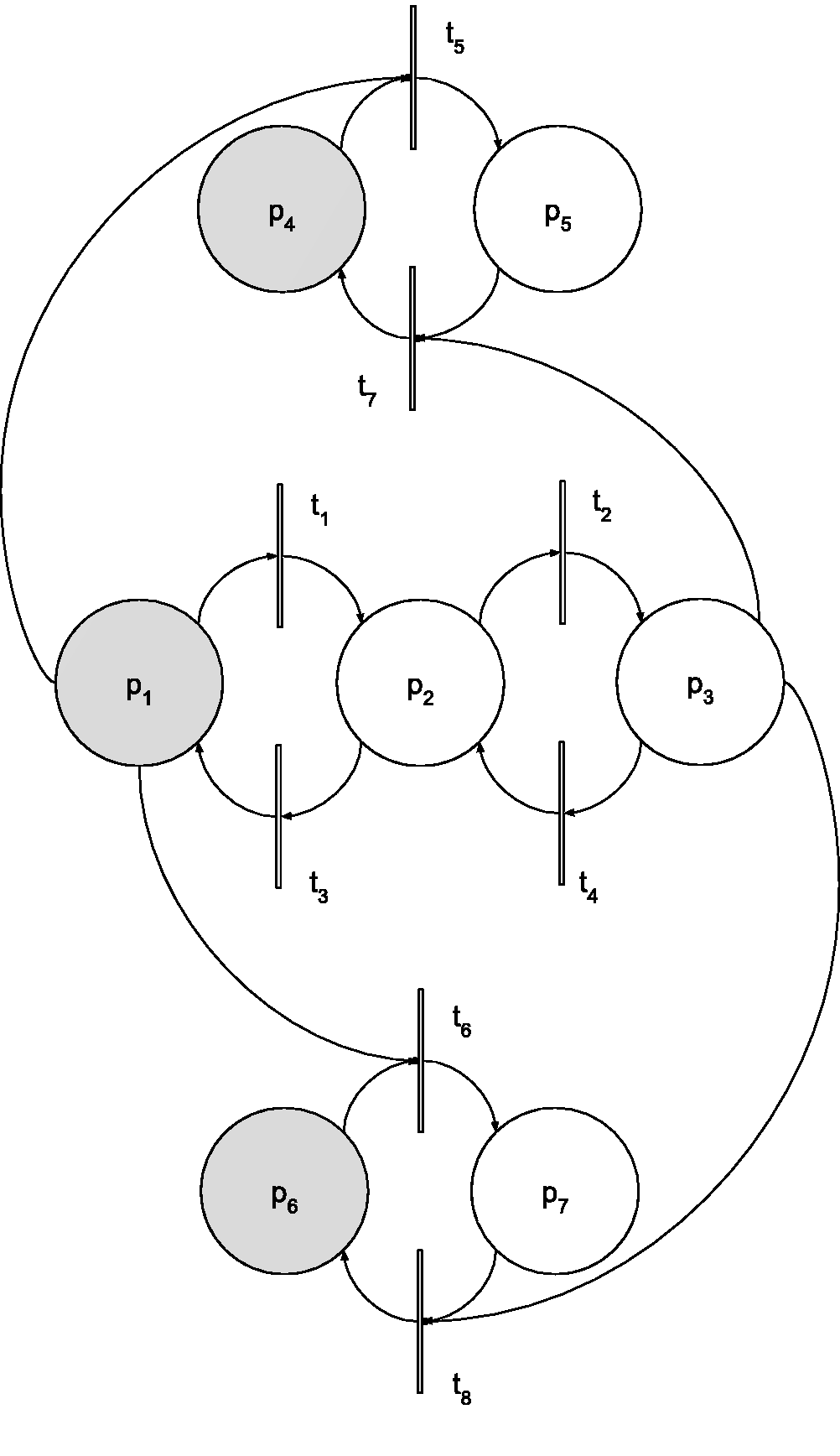
Petri net diagram representing the cup/liquid states of the cup model based on angle {p1,p2,p3}, bottom surface contact {p4,p5}, and top surface contact {p6,p7}. The initial marking {p1,p4,p6} is indicated with gray shading.

An initial marking was set for a vertical cup with the corresponding tokens for this marking reside in places p1, p4, and p6 as shown with shading in Figure 3. Due to the inhibitors, six possible markings result as listed in Table 3. These six markings correspond to the six possible geometric configurations of the liquid within the cup.

Table 3.

Resultant markings for Petri Net model of cup.

Marking	p1	p2	p3	p4	p5	p6	p7
0	1	0	0	1	0	1	0
1	0	1	0	1	0	1	0
2	0	1	0	0	1	1	0
3	0	1	0	1	0	0	1
4	0	1	0	0	1	0	1
5	0	0	1	0	1	0	1

The reachability diagram (Figure 4) shows all possible transitions between markings or geometric states. As drawn, the system behavior transitions from left to right as the cup is tilted from vertical to horizontal (as during drinking). As the cup is tilted back to vertical, the system transitions back to the left. The transition to M2 or M3 is determined by the ratio of the volume of liquid as compared to the cup volume. These particular states will be expanded upon as part of the system model.

Figure 4.

Reachability diagram for the six possible cup/liquid states of the cup.

This representation of the liquid states can be utilized to adjust the controller model based on liquid volume and drinking angle in order to determine the vertical height of the liquid, h_Z. Each marking represents a distinct volumetric geometry. Starting in a static vertical position, M0, the liquid can be represented by a cylinder. As the cup is rotated to M1, the liquid in the cup forms a cylindrical segment (or truncated cylinder). M2 occurs when the volume is small, and the bottom is no longer covered resulting in a cylindrical wedge. Otherwise, state M1 will transition to M3 (liquid contact with the lid). In M3, the air in the cup forms a wedge and the volume of the liquid can be computed by subtracting the air volume from the total cup cylinder. When neither the top or bottom are covered, state M4, a truncated cylindrical wedge results. Finally, the liquid forms a horizontal cylindrical segment when the cup reaches a horizontal position in state M5.

The petri net model formulation directly accounts for contact with the top surface (p7) that contains the drinking aperture. The liquid states represented by M0, M1, and M2 do not contact the top surface and therefore cannot provide liquid to the drinking aperture. Thus, model efficiencies can be obtained since calculation of h_Z in these states is not required.

Determination of liquid shape variables in each state

The controller model requires the dynamic calculation of the liquid shape variables: h_L, x_L, h_T, and x_T in order to monitor the state change events and the liquid height, h_Z, in order to determine if liquid is present at the drinking aperture. The calculations vary in each liquid state. However, the parameters can be directly solved from the volume of liquid, V, the angle of the cup, α, and the cup radius, R_c in each state.

The same equations can be used for the two model states where the liquid is in complete contact with the bottom surface (h_T > 0) and not in contact with the top surface (h_L < h_C). These are model states M₀ (α = 0) and M₁ (0 < α < p/2) and shown in Figure 5. The leading and trailing edge distances are zero in these states ( $x_L=x_T=0$ ).

Figure 5.

Liquid volume geometry in (a) M₀, vertical state and (b) M₁, tilted state.

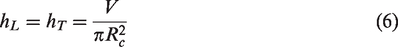
The liquid volume geometry in state M₀ is a simple cylinder and can be rearranged to determine the leading and trailing edge heights as per equation (6).

$$h_L=h_T=\frac{V}{\pi R_c^2}$$

(6)

The liquid volume geometry in state M₁ is a truncated cylinder and the volume is represented by equation (7) which can be rearranged in terms of the leading and trailing edge height variables as per (8) and (9), respectively.

$$V=\pi R_c^2\mathrm{ }\left(\right(h_L-R_C\text{tan}\left(\alpha \right)\left)\right)$$

(7)

$$h_L=\frac{V}{\pi R_c^2}{+R}_C\text{tan}\left(\alpha \right)$$

(8)

$$h_T=\frac{V}{\pi R_c^2}-R_C\text{tan}\left(\alpha \right)$$

(9)

Note that (8) and (9) can be applied for state M₀ where a = 0 and equation (6) results. These liquid shape parameter equations are utilized until h_L or h_T trigger a transition event to states M₂ or M₃.

In state M₂ (Figure 6), the liquid volume forms a cylindrical wedge along the bottom and leading edge of the cup. In this case, h_T and x_L are zero. The height of the wedge equals the leading edge height, h_L. The cylindrical wedge width, b, can be defined in terms of cup system variables by (10).

$$b=2R_C-x_T$$

(10)

Figure 6.

Liquid volume geometry in state M₂.

The volume for a cylindrical wedge can be written in terms of the cup radius, R_c, the cup angle, α, and the width of the wedge, b, per equation (11).

$$V=\frac{\text{tan}\left(\alpha \right)}{6}\mathrm{*}[2\sqrt{2b{R}_C-b^2}\left(3R_C^2-2b\sqrt{2b{R}_C-b^2}+b^2\right)$$

$$-3\pi R_C^2\left(R_C-b\right)+6R_C^2\left(R_C-b\right)\text{sin}\left(\frac{R_C-b}{R_C}\right)]$$

(11)

Furthermore, the cup angle, $\alpha ,\mathrm{ }$ relates the width and height of the wedge by (12).

$$\text{tan}\left(\alpha \right)=\frac{h_L}{b}$$

(12)

In order to compute the incremental changes in the liquid shape parameters, the ratio of the liquid volume to the liquid height, V/h_L, was plotted as a function of the cylindrical wedge width, b, (Figure 7). Based on curve fitting, the relationship is represented by a third order equation of the form:

$$\frac{V}{h_L}=a_0\cdot b^3+a_1\cdot b^2+a_2\cdot b+a_3$$

(13)

Figure 7.

Slope of volume/height as a function of the cylindrical wedge width.

A plot of the coefficients of (13), {a₀, a₁, a₂, a₃}, as a function of the cup radius squared (Figure 8) shows that a linear relationship exists for each coefficient and the cup radius squared of the form:

$$a_i=c_i\cdot R_c^2$$

(14)

Figure 8.

Coefficients, {a₀, a₁, a₂, a₃}, from the 3rd order V/h_L equation as a function of the square of the cylindrical radius, R: a₀ (circle), a₁ (triangle), a₂ (square), and a₃ (diamond).

The resultant equation for the volume of the cylindrical wedge can be written as:

$$\frac{V}{h_L}=(c_0·b^3+c_1·b^2+c_2·b+c_{3\mathrm{ }})R_c^2$$

(15)

Using the relationship between the cup angle, $\alpha ,$ the width and height of the wedge from (12) and substituting for h_L results in a quartic equation in terms of b of the form:

$$\left(c_0·b^4+c_1·b^3+c_2·b^2+c_3·b\right)-\frac{V}{R_C^2·\text{tan}\left(\alpha \right)}=0$$

(16)

Since the liquid volume, the cup angle, and the cup radius are all known, the roots of (16) can be determined. Any complex roots can be ignored and the real root that results in a small incremental change in the liquid shape variables from the last known values can be identified as the next incremental value.

In state M₃, the liquid is touching the top and still in contact with the complete bottom of the cup. The geometry of the liquid does not match any of the standard cylindrical segments (Figure 9). However, the air in the cup is a cylindrical wedge. Therefore, we can use some of the formulation from state M₂. The liquid volume equals the cup volume minus the cylindrical wedge of air:

$$V=-\frac{\text{tan}\left(\alpha \right)\mathrm{ }}{6}[2\sqrt{2b{R}_C-b^2·}\left(3R_C^2-2b\sqrt{2b{R}_C-b^2}+b^2\right)$$

$$\hspace{0.17em}\hspace{1em}-3\pi R_C^2\left(R_C-b\right)+6R_C^2\left(R_C-b\right)\text{sin}\left(\frac{R_C-b}{R_C}\right)+V_C$$

(17)

Figure 9.

Liquid volume geometry in state M₃.

The leading edge height, h_L, equals the height of the cup, h_C. The leading edge distance, x_L, is defined by equation (18) where b is the width of the air wedge. The trailing edge distance, x_T, is zero. The height of the trailing edge is related to the cup height and the width of the air wedge by equation (19).

$$b=2R_C-x_L$$

(18)

$$\text{tan}\left(\alpha \right)=\frac{{h_C-h}_T}{b}$$

(19)

Using (19) and substituting for h_L results in a quartic equation in terms of the width, b, of the form:

$$\left(c_0·b^4+c_1·b^3+c_2·b^2+c_3·b\right)-\frac{V-V_C}{R_C^2·\text{tan}\left(\alpha \right)}=0$$

(20)

Since the liquid volume, the volume of the cup, the cup angle, and the cup radius are all known, the roots of (20) can be analyzed for the real root that results in an incremental change in the liquid parameters from the last known values.

In state M₄, the cup continues to tilt and the trailing edge of the liquid moves onto the bottom of the cup. The resulting geometry is a truncated cylindrical wedge (Figure 10). The trailing edge height, h_T, equals zero and the leading edge height, h_L, equals the cup height, h_C.

$$V=\frac{\text{tan}\mathrm{ }\left(\alpha \right)\mathrm{ }}{6}[2\sqrt{2b_1{R}_C-{b_1}^2}$$

$$\left(3R_C^2-2b_1\sqrt{2b_1{R}_C-{b_1}^2}+{b_1}^2\right)-3\pi R_C^2\left(R_C-b_1\right)$$

$$+6R_C^2\left(R_C-b_1\right)\text{sin}\left(\frac{R_C-b_1}{R_C}\right)-2\sqrt{2b_2{R}_C-{b_2}^2}\left(3R_C^2-2b_2\sqrt{2b_2{R}_C-{b_2}^2}+{b_2}^2\right)$$

(21)

Figure 10.

Liquid volume geometry in state M₄.

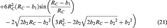
The liquid volume is the difference between an extended cylindrical wedge from the bottom of the cup extended out to an intersection point on the leading edge of the cup and the overlapping wedge from the top of the cup to the same extended point. The height of the extended wedge is denoted by h_E. The relationship between the extended wedge and the liquid state variables is defined by (22) and (23). The relationships for the cylindrical wedge segment from the top of the cup are defined by (24) and (25).

$${\mathrm{b}}_1=2R_C-x_T$$

(22)

$$\text{tan}\left(\alpha \right)=\frac{h_E}{b_1}$$

(23)

$$b_2=x_L$$

(24)

$$\text{tan}\left(\alpha \right)=\frac{{h_E-h}_C}{b_2}$$

(25)

To solve for the leading and trailing edge distances, we can combine (22), (23), (24), and (25) to obtain:

$$b_2=x_L=\mathrm{ }\left(2R_C-x_t\right)-(h_C/\text{tan}(\alpha \left)\right)$$

(26)

Equations (22) and (26) can be combined with (21) to obtain the liquid volume equation in terms of x_T. Once again a quartic equation is obtained with the liquid volume, the cup height, the cup angle, and the cup radius known. The roots can be analyzed for the real root that results in an incremental change in the trailing edge distance, x_T. The leading edge distance, x_L, can be found from equation (26).

In state M₅, the horizontal state (Figure 11), the cup follows the well-established equations for a horizontal cylindrical tank with a length of h_C and a vertical liquid height, h_Z, equal to the leading edge distance, x_L. All of the fluid variables are simply determined. The leading edge is on the bottom of the horizontal cylinder, so h_L = h_C and h_T = 0. The volume equation for a horizontal cylindrical segment is shown in equation (27).

$$V{=h}_C\mathrm{ }[R_C^2\text{cos}{\hspace{0.17em}}^{-1}\left(\frac{R_C-x_L}{R_C}\right)-\left(R_C-x_L\right)\sqrt{2R_C{x}_L-{x_L}^2}]$$

(27)

Figure 11.

Liquid volume geometry in horizontal state M₅.

This can be solved for the leading edge distance, x_L, and then the trailing edge distance can be found from:

$$x_T=2R_c-x_L$$

(28)

In summary, the liquid shape parameters have been determined for each of the geometric shape states. Changes in state are identified as the liquid comes in contact with the different surfaces of the cylinder as defined by the petri net model. Assuming small changes in angle and the resulting shape parameters, a dynamic model of the liquid within the rotating cup has been established. The state based model tracks the shape of the liquid within the cup, (5) provides the liquid height in all states, (2) determines the minimum drinking orifice height in all states, and criterion (4) can determine if liquid is expelled through the drinking orifice at the given orientation. The area of the drinking aperture covered by liquid determined from (4) and (5) can be combined with model time to estimate the differential change in liquid volume in the cup. This model provides a basis for estimating and controlling the flow for a new controlled flow “sippy” cup.

Closed vent modelling

The flow controlled cup is restricting liquid flow based on control of a vent hole valve. The differential pressure from the trapped air when the valve is closed is modelled using Bernoulli’s equation at two locations: the aperture and the air/fluid surface inside the cup.

$$P_{ap}+\frac{\rho }{2}·{v_{ap}}^2+\rho \mathrm{ }gd=P_{\mathit{surf}}+\frac{\rho }{2}·{v_{\mathit{surf}}}^2+\rho \mathrm{ }g{h}_z$$

(29)

When the vent is closed and the aperture is covered with fluid, the air trapped within the cup increases in volume as liquid exits the cup. This creates a decrease in the internal air pressure, 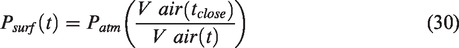$P_{\mathit{surf}}$ , from the time at which the vent was closed. The air pressure inside the cup acts upon the internal exposed surface of the liquid, $A_{\mathit{surf}}$ . Atmospheric pressure, $P_{\mathit{atm}}$ , is still acting on the liquid at the drinking aperture with area, $A_{ap}$ . The change in internal pressure is defined by equation (30).

$$P_{\mathit{surf}}\left(t\right)=P_{\mathit{atm}}\left(\frac{V\mathrm{ }\mathit{air}\left(t_{\mathit{close}}\right)}{V\mathrm{ }\mathit{air}\left(t\right)}\right)$$

(30)

Due to conservation of volume, the volumetric flow rates at both points are equal and can be defined by the velocity and area at each location.

$$Q_{ap}=Q_{\mathit{surf}}$$

(31)

$$v_{ap}\mathrm{\hspace{0.17em}*}\mathrm{\hspace{0.17em}}{A}_{ap}=v_{\mathit{surf}}\mathrm{*}{A}_{\mathit{surf}}$$

(32)

Rewriting Bernoulli’s equation in terms of the aperture exit velocity, $v_{ap}$ , and then substituting values from (30) and (32), equation (34) is obtained as a function of time.

$$v_{ap}=\sqrt{\frac{2}{\rho }[\left(P_{\mathit{surf}}-P_{ap}\right)+\rho \mathrm{ }g\left(h_z-d\right)+\frac{\rho }{2}·{v_{\mathit{surf}}}^2]}$$

(33)

$$v_{ap}\left(t\right)=\sqrt{\frac{2}{\rho }·P_{\mathit{atm}}·\left(\frac{V\mathrm{ }\mathit{air}\left(t_{\mathit{close}}\right)}{V\mathrm{ }\mathit{air}\left(t\right)}-1\right)+\frac{2g\left(h_z-d\right)}{1-{(A_{ap}/A_{\mathit{surf}})}^2}}$$

(34)

It is noted that the head above the aperture is defined by the liquid height, h_z, and the height to the center of the drinking aperture, d, and must be a positive value to maintain liquid covering the aperture. The relationships in (32) and (34) can be used to estimate the volumetric flow rate from the aperture when the vent is closed. The cup is designed to maintain a desired volumetric flow rate to meet the needs of the individual utilizing the cup.

Cup flow control

The cup controller regulates the fluid flow by on-off control of the vent valve. When the vent is open, the fluid can flow freely from the drinking aperture. A closed vent hole reduces flow until the exit velocity reaches zero. Pulsed control of the vent valve can regulate the flow between the free flow rate and zero.

Cup sensors monitor the time varying drinking angle, a, and the weight of the fluid, w, throughout rotation. It is assumed that the cup prototype uses two force sensitive resistors between a floating inner cup and an external cup shell to measure the axial and radial components of the weight which will provide w. It is assumed that the type of fluid is known and the fluid density is available for the fluid model. The fluid model accounts for the time varying behavior of the fluid variables and the related changes in geometric system states while estimating the current flow rate. As the estimated flow rate exceeds the desired flow rate, the vent valve is actuated to adjust the open/close time ratio (Figure 12).

Figure 12.

Block diagram for cup control scheme.

Model implementation

The model was implemented in a controlled flow cup simulation which will support development through a visual user interface and integrate physical prototyping. This framework is being implemented through the open source development tools Processing and Arduino. The cup flow model implementation in Processing provides a 2 D visualization of the cup geometry, a visual display of the cup and liquid parameters, and generates a data file of the cup and liquid parameters for the simulated run. The input parameters (Table 4) can be modified to test different cup and liquid conditions. The model can estimate the flow rate for a child drinking a specified amount of liquid at a specified viscosity from a particular cup geometry while tipping the cup at a particular rate. These were implemented with new cup and liquid classes. In order to implement the model, the following programming structure was utilized (Figure 13). The geometry based model presented in the Determination of leading edge height of liquid section, the Petri net model of liquid states section and the Determination of liquid shape variables in each state section is implemented in the liquid class utilizing the cup class parameters. The flow control model from the Closed vent modelling section and the Cup flow control section is implemented in the controller code.

Table 4.

Simulation parameters for classes associated with the cup and the liquid.

For liquid class:	For cup class:
liquid volume	cup height
density	cup radius
initial height of liquid	drinking aperture diameter
leading edge height	drinking aperture distance from rim
leading edge distance from the rim	vent hole diameter
trailing edge height	vent hole distance from rim
trailing edge distance from the rim	cup volume
liquid level in vertical direction	drinking aperture max in vertical direction
	drinking aperture min in vertical direction
	drinking aperture area

Figure 13.

Program structure for cup flow model.

As the model increments the time, all cup and liquid parameters are saved to a data file. The time dependent liquid shape variables are utilized to generate a polygon in the 2 D plane that shows the rotation of the cup. The visual depiction of the liquid shape is displayed on the screen to provide a cross sectional side view of the cup and liquid as the drinking angle progresses (Figure 14).

Figure 14.

The 2 D visualization of the cup model progressing from a vertical to a horizontal state.

Simulation case study

To demonstrate the simulation model, a sample run was conducted based on typical transitional cup drinking conditions that we have recorded in the Miami University Dysphagia lab. The cup size and liquid volumes are consistent with those of a child transitioning to an open-cup. The cup capacity is approximately 340 ml. The liquid volume is 200 ml of water, leaving a volume of approximately 140 ml of air in the cup. The simulation progresses at 0.01 s increments which is sufficient to capture changes as they would affect transitional drinking behavior. The cup transitions from 0 to 90 degrees in 2 seconds which results in a rate of 0.785 rad/s or 45 deg/s. The simulated conditions for this run are presented in Table 5.

Table 5.

Simulated conditions for a transitional cup drinking scenario.

Variable	Measure	Units
time increment	0.01	s
cup height	12	cm
cup radius	3	cm
drinking aperture diameter	0.5	cm
drinking aperture distance from rim	0.5	cm
vent hole diameter	0.1	cm
vent hole distance from rim	0.5	cm
liquid volume	200	ml
liquid density	1	g/ml
angle velocity	45	deg/timestep

The case study demonstrates two conditions: free flow and controlled flow with a desired rate set point of 5 ml/s and pulse width modulation with a period of 1 second and a 50% duty cycle. Both simulation cases progress until the liquid stops pouring from the cup.

Results

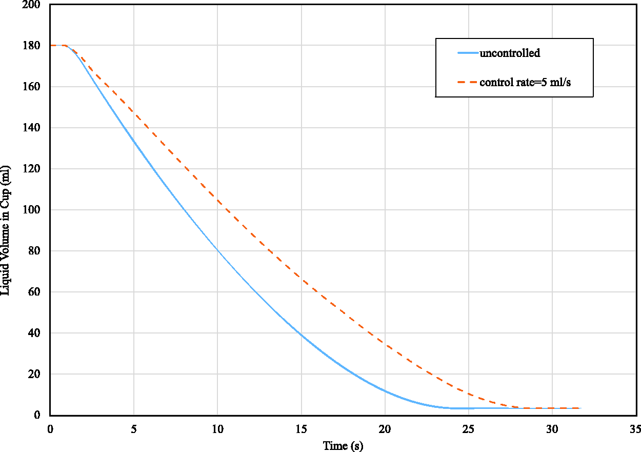
The simulation provides the user with a two-dimensional visualization of the draining cup and a numerical output file of key variables. A subset of the numerical output from the free flow case is presented in Table 6. A progression of the visualization for the free flow case is shown in Figure 14. The left image displays the cup just after rotation has been initiated and the full volume of the liquid remains in the cup. The middle image shows the liquid level just after the drinking aperture has been reached and the liquid level is starting to decrease. The right image shows the cup in a horizontal state as the liquid is pouring out of the cup and the angle is no longer progressing.

Table 6.

Sample simulated output data from free flow of water.

Time (s)	15.00025
Angle (rad)	1.570796
Water volume (ml)	66.43544
Air volume (cm3)	173.8388
Volumetric flow rate, Q (ml/s)	5.755077

The liquid volume in the cup and the cup angle as a function of time for a cup starting at rest in a vertical position and rotated to a horizontal position are presented in Figure 15.

Figure 15.

Liquid level and cup angle as a function of time for free flow.

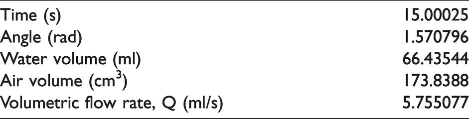
From this baseline case, alternate cases were run to demonstrate the ability of the model to capture different cup dynamics, liquid conditions, and controller settings. Therefore, cases were run to study the effects of varying rotation rates, initial volume, and desired flow rates. The results from uncontrolled as compared to controlled flow are displayed in Figure 16. The results for varying rotation rates are displayed for the first 5 seconds of the simulation run in Figure 17. The initial volumes were varied from 120 ml to 210 ml in 30 ml intervals and the resulting flows as a function of time are presented in Figure 18. In order to study controller effects, the desired flow rate was set at 1 ml/s, 5 ml/s, and 50 ml/s and the resulting flow versus time behavior is plotted in Figure 19.

Figure 16.

Liquid volume in the cup as a function of time for free and controlled flow at a desired rate of 5 ml/s.

Figure 17.

First 5 seconds of liquid volume in cup as a function of time. Rotation time was set to vary: 1 sec, 2 sec, and 4 sec. Flow rate fixed at 5 mL/sec with varying rotation rate of the cup from 0 to 90 degrees. Y axis: liquid volume in cup (mL), X axis: time (sec).

Figure 18.

Liquid volume in the cup as a function of time for varying initial volumes. Flow patterns are based on initial volume levels of 120 ml, 150 ml, 180 ml, and 210 ml. The desired flow rate was fixed (5 ml/sec) with a rotation time of 2 seconds from 0 to 90 degrees.

Figure 19.

Liquid volume as a function of time for varying flow rates. Graph represents the change in flow patterns based on select flow rates. Chosen flow rates included: 1 mL/sec, 5 mL/sec, and 50 mL/sec. Initial volume was fixed (180 mL) with a rotation rate of 2 seconds from 0 to 90 degrees.

Discussion

The simulated results display the expected behavior of a pouring fluid as different parameters are varied. The baseline curve for the volume remaining in the cup as a function of time (Figure 15) shows the expected decrease in the rate of the liquid flow as the volume in the cup and the resulting head is reduced. The free flow of a fluid from a cup will start out at a faster rate when there is a larger volume of liquid above the drinking aperture. As this volume decreases, the rate decreases which is evidenced by the slope of the curve This graph also shows how that flow starts during rotation as the liquid reached the drinking aperture. This captures a realistic behavior of a child tipping the cup until liquid would reach the drinking aperture and then flow. For the simulated cup, the drinking aperture is 0.5 cm from the edge of the cup. Once the liquid has covered the drinking aperture, liquid continues to flow until the liquid level falls back below the drinking aperture resulting in some residual fluid in the cup. This resulting residual fluid matches the physical behavior of the cup/liquid system.

The effect of the controller function is demonstrated in the difference in flow rates exhibited in Figure 16. The flatter curve represents the more consistent flow of the controlled cup as compared to the variation in slope (or flow rate) of the free flow curve. When the instantaneous flow rate exceeds the desired flow rate of the cup, the controller closes the vent hole which creates a vacuum in the cup as the liquid flows from the drinking aperture. As the negative pressure builds within the cup, the flow will slow down, resulting in a delayed response to the restriction of the flow. The flow from the controlled cup is reduced relative to the uncontrolled cup. However, the resulting controlled rate is less than the desired flow rate of 5 ml/s which would require 36 seconds to drain the 180 ml initial volume. In order to investigate the effect of the desired flow rate, simulated runs with desired flow rates of 1, 5, and 50 ml/s were simulated. The resulting remaining liquid volume as a function of time curves in Figure 19 show the expected reduction in flow for the lower flow cases. The flattest curve results from the lowest set rate for the controller. The 50 ml/s case does not restrict the flow as this desired rate is higher than expected flow rates for uncontrolled flow.

The model was tested for different rotational rates which would simulate the variation in users rotating the cup. The results for three different rates based on rotations times from vertical to horizontal of 1, 2 and 4 seconds are presented in Figure 17. The model updates the cup angle, modifies the liquid shape, and then detects the initiation of flow at the drinking aperture. The resulting delay in fluid flow resulting from slower cup rotation is seen in the results. The rotational rate is no longer a factor in fluid flow after the cup reaches horizontal.

Variations in initial liquid volume were tested and the results in Figure 18 display the different volume in the cup as a function of time. Lower initial volumes result in a lower head level once the cup has reached horizontal. Therefore, initial flow rates are expected to be lower for the lower volume cases. The model captures the behavior of a mostly full cup showing the faster flow of the liquid when it firsts reaches the drinking aperture.

Conclusions and future work

A novel model has been presented to uniquely capture the fluid flow for a rotating cup. The model formulation has shown that the definition of new liquid shape variables can directly identify the geometric states of the system through a Petri Net formulation of the system states. This model is limited to a cylindrical vented cup with vent control and in plane rotation toward the drinking aperture.

The model provides the basis for investigating many factors that affect transitional drinking in children. The model can be implemented in a microcontroller based prototype cup implemented with Arduino code directly modified from the Processing code. Future work will compare simulated results with experimental results from a physical prototype running the model and obtaining feedback from sensors integrated in the cup.

The model facilitates the investigation of the vent hole based flow control scheme. The model captured the lag that occurs as the vacuum accumulates in the cup cavity. Therefore, the relationship between the desired flow rate and the resulting flow rate from simulated and experimental systems will be investigated which can be used to tune the physical controller.

A key element of the model is that liquids are implemented as a class. Transitional drinking typically uses water, juices, milk, yogurt drinks and formulas. Whereas density is already accounted for in the existing model, the effect of viscosity on the system is undetermined. Future work will investigate the flow properties of these liquids and determine the most effective way to implement these in the model and the prototype controller.

In a similar manner, the model implements the cup as a class. Different cup geometries can be quickly simulated. This will assist in the determination of the cup geometry for the physical prototype. Key factors are variation in the location and size of the vent hole and drinking aperture. This new model will reduce the development phase for designing the prototype transitional drinking cup.

Future work will also focus on the prototyping of the device based on model outcomes. This work will investigate the accuracy of physical flow behavior in relation to the model outcomes. Furthermore, prototyping will investigate the cost to performance relationship of the device.

Identifying effective drinking behaviors as children transition to open cup drinking is facilitated by the new cup and liquid based model. The model verification results were based on a rotation from a vertical to a horizontal position. Future work will enable more complex drinking motions to be simulated by using a time varying profile of the angle. These profiles can be generated from observational data obtained from children drinking from various cups with various volumes. The simulation of these drinking behaviors will provide insight into the proper cup-liquid-flow control to promote positive drinking behavior as children transition to open cup drinking. The ultimate goal of developing this new technology is to serve the largest number of users who have difficulty swallowing liquids.